Proof methods for reasoning about possibility and necessity

Proof Methods for

Reasoning About

Possibility and

Necessity

Churn Jung Liau

Institute of Information Science, Academia Sinica, Taipei, Taiwan, R O C

Bertrand I-Peng Lin

Department of Computer Science and Information Engineering, National Taiwan University, Taipei, Taiwan, R O C

ABSTRACT

Possibilistic logic is a quantitative method for uncertainty reasoning that is closely related to Zadeh's fuzzy set theory. In this paper, we formulate it as a kind of multimodal logic and develop some proof methods for it, including tableau method and two styles of natural deduction methods. The completeness and soundness of these methods are proved. Finally, some potential applications and the possible research directions are pointed out.

KEYWORDS:

Fuzzy set, possibilistic logic, modal logic, Kripke semantics,

tableau method, natural deduction method

1. INTRODUCTION

In the last 30 years, many uncertainty reasoning schemes have been proposed by logicians, scientists and engineers. Among them, possibilistic logic, which is proposed by Dubois and Prade [1] and is closely related to Zadeh's fuzzy set theory [2], is one of the most important approaches. The logic arises naturally in the following scenario [3].

Address correspondence to: Bertrand 1-Peng Lin, Department of Computer Science, National Taiwan University, Taipei, Taiwan, ROC.

Received March 1, 1992; accepted March 19, 1993.

International Journal of Approximate Reasoning 1993; 9:327-364 © 1993 Elsevier Science Publishing Co., Inc.

328 Churn Jung Liau and Bertrand I-Peng Lin Consider a state-descriptive information system (SDIS)

~ = (U, PV>,

where U is the set of all possible states of the world under consideration, and

PV

is a set of propositional variables that describe some things about the world. For each u ~ U, assume that u is complete with respect to

PV

in the sense that for each

p ~ PV, p

is either true or false under the state u, we will write

u(p)

= 1 (resp. = 0) if p is true (resp. false) under state u. Then, the

truth set

of the proposition p, written as Ip[, is defined as the set of all states u such that

u(p)

= 1. Let us define a

query formula f

to the SDIS as a Boolean combination of the propositions in

PV.

The truth value of f under a state u is completely determined by the classical logic truth table and the truth values of the propositional variables under u. Thus, the definition of the truth set can be extended to any queries accordingly.

Now, if a piece of fuzzy information is stored in the SDIS, then the truth value of a formula f can be determined according to the stored informa- tion. A piece of fuzzy information /x is defined as a fuzzy subset (i.e., a possibility distribution) of U. Formally, Iz: U ---, [0, 1] is a piece of fuzzy information. The fuzzy information /~ is called normalized iff SUpu ~ v /z(u) -- 1. In general, we require the fuzzy information is normalized. In this case, two measures II and N: 2 U ~ [0, 1] are defined as follows,

f l ( X ) = s u p / z ( u ) u E X

N ( X )

= 1 - I I ( U \ X ) .

Let I I ( f ) = H(Ifl) and

N(f)

= N(Ifl), then the following properties hold for all formulas f , f l , and f2:

(i) I I ( f ) and

N(f) ~

[0, 1] ( i i )

N(f)

= 1 - I I ( - ~ f ) ,

(iii) II( 7- ) = 1 and II( _1_ ) = 0, and (iv) I I ( f l V

fz)

= max(H(fl), H(fz)).

By attaching two measures to classical logic formulas, possibilistic logic is obtained. More specifically, if f is a well-formed formula (wff) of propositional logic, then

( f ( N c))

and ( f ( H c)) where c ~ [0, 1] are wffs of possibilistic logic. When f is a classical clause, the wffs are called possi- bilistic clauses. The intended meanings of the wffs are

N(f)>_ c

and H ( f ) >__ c respectively. Then, the resolution rule of possibilistic logic is defined between two possibilistic clauses as follows:

(fwO (g w2)

( / { ( f , g ) W 1 * W2)

Proof Methods for Reasoning 329 where

R(f, g)

is the classical resolvent of f and g, and * is defined by

(N c ) * ( N d) = (N

m i n ( c , d ) )

( N c ) * ( I I d )

= / ( I I d ) i f c + d > 1

(II0)

i f c + d < l

(II c ) * ( I I d) = (II 0)

By the axiom (iv) above, any wff of the form

(f(Nc))

can be converted into an equivalent set of possibilistic clauses, so if only necessity measure N is concerned, the refutational completeness of this resolution rule can be proved [3]. However, if possibility-valued wffs are involved, then the completeness result does not hold in general. The following simple example will explain this point further.

EXAMPLE 1.1 Consider the assumption set B -- {(p /x q(H 0.7), ( p / x q

r(N

0.6))} and the wff f = (r(II 0.7)) in possibilistic logic. Then obviously, f should be derivable from B. t However, since ( p / x q(II 0.7)) is not a possibilistic clause, the resolution rule cannot be applied. A possible approach to overcome the difficulty may be to infer (p(II 0.7)) and (q(II 0.7)) first. This indeed improves on some situations if the second sentence is either (p ~ r (N 0.6)) or

(q ~ r(N

0.6)), but it is useless for the present example.

To lift the restriction of clausal form, we must consider more general deduction methods. Some non-clausal deduction methods for modal logics have been well studied by Fitting [4], so by formulating possibilistic reasoning as a kind of multimodal logic, we can generalize Fitting's methods to possibilistic logic. Recently, some modal formulations of possi- bilistic logic have been proposed [5, 6]. Here, we will review one of them, called quantitative modal logic (QML), and develop some nonclausal deduction methods for it. These include tableau methods and natural deduction methods.

In what follows, we will first review the syntax and semantics of QML. Then the advantages of QML in possibilistic reasoning is discussed. A basic theorem for the completeness of QML deduction methods, called model existence theorem, is proved in section 3. The above-mentioned proof methods are presented in section 4 and 5 sequentially. Finally, some related works are discussed and a brief conclusion is given.

1Replacing "p A q" with a new propositional letter and using the given resolution rule will justify this.

330 Churn Jung Liau and Bertrand I-Peng Lin

2. QUANTITATIVE MODAL LOGIC

2.1. Syntax

To define a new logical language, we must specify its syntax and semantics.

First, the alphabet of Q M L consists of logical constants, connectives and a (denumerable) set of propositional variables.

• Logical constants: T

(verum

or

truth constant)

and _1_

(falsum

or

falsity constant).

• Propositional variables: p, q, r , . . . , etc.

• Classical connectives: --7 (negation), v (or), A (and), and (implication).

• Quantitative modal operators: [c], ( c ) , [c] +, and ( c ) + for all c

[0, 1]. 2

Second, the well-formed formulas

(wffs)

of Q M L are defined by the following recursive syntactic rules:

• all propositional variables and logical constants are wffs, also called atomic formulas,

• if

fl

and f2 are wffs, so are -~ f l ,

fl A f2, fl V

f2, and f l

D f2,

• if f is a wff, so are [c]f, ( c ) f , [c]+f, and

(c)+f

for all c E [0, 1], • expressions except those determined by above are not wffs.

We usually use lowercase letters (sometimes with indices) p, q, r to denote atomic formulas and f , g, h to denote wffs. In the present case, wffs are also called sentences. Parentheses are punctuation symbols used to avoid ambiguity in the formation of wffs. The formula

" f - g"

is taken as an abbreviation of " ( f ~ g) A (g ~ f ) . "

Now, we introduce some notations which will be used later. DEFINITION 2.1

Let S be a set of wffs. Then

1. Define the positive subformula set of S, denoted by S +, as the smallest

set containing S and being closed under the following conditions:

(a) if ~ f, (c)f, (c) +f,

[c]f,

or

[ c ] + f ~

S +, then f ~ S +.

(b) i f f Ag, f V g, f D g ~ S + , t h e n f , g ~ S +.

2. Define the negation subformula set of S, denoted by S-, as the

following set:

S - = { ~ f l f ~ S + } .

2Here, c is in fact a numeral designator representing a real number in [0, 1], not a number itself. However, we will not distinguish a number from the symbol representing it rigorously. Furthermore, to keep the language countable, we may restrict c to be a rational number. However, the results we will present still hold without such restriction.

Proof Methods for Reasoning

Table 1. a Wffs and Their Component Formulas

331 0/ 0/1 0/2 f a g f g ~ ( f v g) --~f ~ g -~(f Dg) f -~g -7-~f f f

3. Define Sub(S) = S+U S-.

4. Define the parameter value set of S, V(S) as follows:

V(S) = {c,1 - c [3f such that [c]f, ( c ) f , [ c ] + f , or

( c ) + f ~ Sub(S)} U {0,1}.

Also, Sub(f) = Sub({f}) and V ( f ) = V({f}) if f is a single wff. Note that if S is finite, then Sub(S) and V(S) are, too. Furthermore, an atomic wff or its negation is called a literal.

Following the ideas in [4], we may classify the non-literal wffs of Q M L into six categories according to the formula's main connective that is used to combine its direct subformulas. The classification will simplify the presentation of definitions and theorems in section 3. We list the six categories of wffs and their corresponding subformulas in Tables 1-4. In each table, the original wffs appear in the left of the vertical line and their corresponding subformula(s) in the right. For example, a wff of the form ~ ( f v g) is an a-formula, and its two components, called a I and a2, are f and -1 g respectively, while a wff -~[0.4]+p is a Ir(0.6)-formula, and its component, called Ir0(0.6), is ~ p.

2.2. Semantics

Here we consider the semantics of QML. Define a possibility frame F = (W, R ) , where W is a set of possible words and R: W 2 ~ [0, 1] is a fuzzy accessibility relation on W. Let P V and FA denote the set of all propositional variables and the set of all wffs respectively. Then a model of Q M L is a triple M = (W, R, TA), where (W, R ) is a possibility flame and

Table 2. /3 Wffs and Their Component Formulas

/3 /31 /32

f v g f g

~ ( f Ag) ~ f ~ g

332

Table 3.

v(c)

~ ( l[c_]fc ),+f

Churn Jung Liau and Bertrand I-Peng Lin v and v + Wffs (with P a r a m e t e r c) and Their

C o m p o n e n t Formulas

Vo(C)

v+(c)

v~(c)

f

[c]+f

f

~ f ~<1 - c ) f ~ f

TA: W × P V -o {0, 1} is a truth value assignment for all worlds. A proposi-

tion p is said to be true in a world w iff TA(w, p ) = 1. Given R, we can define a possibility distribution Rw for each w ~ W such that Rw(s) =

R(w, s) for all s ~ W. Similarly, we can also define TA w for each w ~ W

such that TAw(p) = TA(w, p ) for all p ~ PV. Thus, mathematically, a model can be equivalently written as (W, (Rw, TAw )w ~ w ), and intuitively,

TA w describes the ontological state of the world w, while R w reflects the

epistemic state of the world w.

Given a model M = ( W , R , TA), we can define the truth rela- tion ~M C_ W X FA as follows. First, for each world w and wff f , let H w ( f ) = s u p ~ w{Rw(s)ls ~M f} and N w ( f ) = 1 - Hw(-~ f ) (1) W ~M P ~ TA(w, p ) = 1, Vp ~ PV, (2) w ~:::::M "]- and w ~¢:M I , (3) w ~M ~ f "=" w ~:M f , (4) w [:::::M f A g ~, w ~M f and w I::::: M g, (5) w ~M f V g ¢* w ~M f or w ~M g' (6) WWM f D g ~ W ~ M ~ f ° r WWM g, (7) w ~M ( c ) f ¢~ H w ( f ) > c, (8) w ~M ( c ) + f ¢* H w ( f ) > c, (9) w ~M [ c ] + f ¢~ N w ( f ) > c, (10) w ~M [ c ] + f ¢~ Nw(f) > c.

Clauses (7)-(10) define the meaning of wffs with modal operators. Intu- itively, [c]f (resp. [ c ] + f ) means that N ( f ) > c (resp. N ( f ) > c), and similarly, ( c ) f (resp. ( c ) + f ) denotes that I I ( f ) > c (resp. I I ( f ) > c). Here, for convenience, we define sup O = 0 and inf Q = 1.

A wff f is said to be valid in M = (W, R, TA), written ~M f iff for all w ~ W,W~M f. If S is a set of wffs, then ~M S means that for all

Table 4. 7r and ~-+ Wffs (with P a r a m e t e r c) and Their C o m p o n e n t Formulas

~'(c)

%(c)

( c > f f ~[1 -

c]+f

~ f

~'+(c)

~(c)

(c) +f

f

- , [ 1 -

c]f

-~f

Proof Methods for Reasoning 333 f ~ S, ~ u f- If C is a class of models and S is a set of wffs, then we write S ~c f to mean that for all M ~ C, ~M S implies ~M f. A model with finite possible worlds is called finite model. A model is called serial iff for all w in W, sups ~ w R(w, s) = 1, and reflexive iff for all w in W, R(w, w) =

1. Throughout this paper, we use K, D, and T to denote the class of all models, serial models, and reflexive models. If C is a class of models, then FC denote the class of all finite models in C. We also note that T _ D c K.

We can also see from the semantics that the main difference between QML and possibilistic logic is the former allow different possibility distri- butions for each world w, that is Rw, while the latter associate a constant possibility distribution to all worlds. Thus, we have enhanced the expres- sive power of standard possibilistic logic. For example, if from some information source, we get a rule "Smoking implies the possibility of cancer being at least 0.8," but the certainty (necessity) of the rule is at most 0.7 due to the realiability of the information source, then we can represent this fact as ~[0.7]+(p ~ (0.8)q), where p and q denote "smok- ing" and "being cancered" respectively. Furthermore, the syntax makes it easier to combine QML and other intensional logic. For instance, we can use B(0.6)p and (0.6)Bp to represent "the agent believes that the possibility of p is at least 0.6" and "the possibility of the agent believing p is at least 0.6" respectively. Recently, a complete axiomatic QML system for reasoning about higher order uncertainty has also been proposed [7]. This shows that QML has indeed some advantages on the representation of complex uncertainty wffs.

2.3. QML and Possibilistic Reasoning

To understand the relation between QML and possibilistic logic, we first show that all axioms for possibilistic logic can be realized in all serial models in the following sense.

THEOREM 2.1 (1) ~K [0]f A -~[1]+f A <0)f A ~ < l > + f (2) ~K ([c]f A -7[c]+f) -- ((1 -- c > ~ f A ~ ( 1 -- c) + ~ f ) (3) ~o ( 1 ) T and ~ ~ ( 0 ) + ± (4) ~K ([c](f A g) A -~[c]+(f A g)) - ([c]f A -~[c]+f A [c]g) V ([c]g A ~[c]+g A [c]f)

Proof The proof is nothing more than a direct expansion according to

the above-defined semantics. []

Since D c K, Theorem 2.1 is valid in all serial models. According to the possible-world semantics, Theorem 2.1. exactly corresponds to the four axioms for possibility and necessity measured in Section 1. Note that

334 Churn Jung Liau and Bertrand I-Peng Lin Theorem 2.1. (4) says that N ( f /x g) = c iff ( N ( f ) = c and N ( g ) >_ c) or

( N ( g ) = c and N ( f ) >_ c), i.e., N ( f A g) -- c iff m i n ( N ( f ) , N ( g ) ) =

c, which is equivalent to say that I I ( f v g ) = max(II(f), II(g)), since

N ( f ) = 1 - II(-~ f ) . Thus, the consequence relation in serial models is exactly suitable for possibilistic reasoning. But how about K and T? Recall that we can define a possibility distribution R w for each world w in a possible world model according to its accessibility relation R, then the seriality of a model is equivalent to the normalization of all its correspond- ing possibility distribution. 3 Since the normalization requirement is what Dubois et al. [8] impose on the semantics of possibilistic logic, the conse- quence relation in K is just the result of lifting this constraint. Thus, though the consequence relation for K is too weak for possibilistic reason- ing, it can tell us which theorems of possibilistic logic may be derived without the normalization requirement. As for T, since all reflexive models are also serial, we can do possibilistic reasoning by ~T" However, why the stronger consequence relation ~T is useful? To understand this, let us generalize the notion of reflexivity. Given e ~ [0, 1], we define a model

( W , R , T A ) as e-reflexive iff Vw ~ W, R ( w , w ) > e. We then have the following axiom A X T e which is valid in all e-reflexive models.

AXT~: [1

-

e]+fDf

In general, A X T 1 e is called e-threshold axiom. It is named so because we accept a wff as true when its necessity measure is greater than e. Then AXT1, the strongest threshold axiom, i.e., 0-threshold axiom, is valid in all reflexive models. Although the results we will present for T may be generalized to any e-reflexive models, to keep simplicity and facilitate the comparison with ordinary modal logic, we will prove these results in T directly.

3. MODEL EXISTENCE THEOREM

The model existence theorem provides a powerful tool to the proof of completeness for many formal systems, in particular, for those without compactness, such as the infinitary logic L~o~o , [9]. Fitting first gives a systemic presentation of the model existence theorem for modal logic, and proves many important results using this theorem [4]. Interestingly, by modifying Fitting's argument, many results for ordinary modal logic may be transferred to Q M L without too much distortion.

Proof Methods for Reasoning 335 The central idea of the model existence theorem is the so-called consis-

tency property. To define it, we need the following functions. Throughout

this section, let F = Sub(G) for some finite set of wffs, G. Also recall the notation V ( F ) from Section 2, and let a,/3, v(c), v+(c), 7r(c), ~'+(c) denote a wff in the corresponding categories respectively.

DEFINITION 3.1 Define the world-alternatiue function K and strict world- alternatit,e function K + on F as follows.

K, K+: 2 F × V ( F ) --, 2 F, K ( S , c ) = (Vo(C')lc' > c, v ( c ' ) ~ S} u { v ; ( c ' ) l c ' >_ c, v+(c ') e S} and K + ( S , c ) = {Vo(C')lc' > c, v ( c ' ) ~ S} U { v; ( c ' ) l c ' >__ c, v + (c ') ~ S}.

Intuitively, K(S, c) (resp. K+(S, c)) contains all wffs f such that N ( f ) >_ c (resp. N ( f ) > c) can be derived from S by using only duality property of N and II (i.e., axiom (ii) of Section 1) and the transitivity of inequality relation.

DEFINITION 3.2 Let 0 c 2 F be a collection of subsets o f F . Then (1) O is called a classical consistency property of F iff for all S E O, S

satisfies the following three conditions: (a) a e S. ~ S U { a l , Of 2} ~ 19,

(b) / 3 ~ S ~ S U { / 3 1 } ~ 1 9 , o r S U { / 3 2 } ~19, and

(c) for any atomic wff p, S does not contain p and -7 p simul-

taneously, and none of the following wffs are in S: v+(1),

~-+(1), -~ T , J_.

(2) A classical consistency property 19 is a K-consistency property iff for

all S ~ 19, S satisfies, in addition to (a)-(c), the following two

conditions:

(kl) c > 0 and ~ ( c ) ~ S ~ K+(S, 1 - c) U {Tr0(c)} ~ 19, and (k2) 7r+(c) ~ S ~ K(S, 1 - c) U {Tr;(c)} ~ 19.

(3) A T-consistency property is a K-consistency property with the follow-

ing condition:

(t) VS ~ ® , f ~ K + ( S , O ) ~ S u {f} ~ (9.

(4) A D-consistency property is a K-consistency property with the follow-

ing condition:

(d)L VS ~ 19, K+(S,O) ~ 19.

Let B _ F and L = K, T or D, then an L-consistency property ® is called B-compatible iff for all S ~ 19, and f ~ B, S u {f} ~ 19.

336 Chum Jung Liau and Bertrand I-Peng Lin It can be checked that for any wff f, if f ~ F, then the corresponding component formulas fl and f2 (in the case of f being a o r / 3 wff) or f0 (in the other cases) are all in F by the requirement of F = Sub(G). This simple fact is critical to the well-definedness of the consistency property since we require that O is a subset of 2 e.

Obviously, the consistency property is closely related to the satisfiability of wffs. The intuition is formally stated as the following theorem. However, before the presentation of the main theorem, let us illustrate these definitions with a simple example.

EXAMPLE 3.1 If O is a K-consistency property and S = {(0.7)pl,

[0.4]p2, [0.3]+P3}

~ O,

then from the consistency of S, we can infer that there is a model M = ( W , R, T A ) and a world w ~ W such that w ~ S. Since w ~ (0.7)pl, under the assumption that W is finite (an assumption which can be made without loss of generality by Corollary 3.1.), there exists another world u such that R ( w , u) > 0.7 and u ~ Pl. Now, because w ~ [0.4]p2 A [0.3]+P3, we have Nw(p2) > 0.4 and Nw(P3) > 0.3, i.e., IIw(--np2) < 0.6 and

I-Iw(--np3) <

0.7, so for u ~ W such that R ( w , u ) >

0.7, we have u ~ P2/x P3- Thus, u ~ K ÷ ( S , 0.3) U {Pl} since K ÷ ( S , 0.3) = {P2, P3}. That is, K ÷ ( S , 0.3) U {Pl} should be also consistent. This explains the (kl) condition of definition 3.2(2). Other conditions of consistency properties can be explained essentially in the same way.

THEOREM 3.1 (Model Existence Theorem) Let L = K, T, or D. I f F is finite, B c_ F, and 19 is a B-compatible L-consistency property on F, then there exists a finite model M = (IV, R, T A ) in L such that ~M B and f o r all f ~ S ~ O, there exists a world w ~ W such that w ~ f .

Proof To prove this theorem, we use a constructive argument. First, noting that O is ordered by __c_ and all elements of O is finite sets, we can construct the model M o = (IV, R, T A ) as follows:

W: the set of maximal members in O,

TA(S, p ) = 1 ~, p ~ S, V S ~ W and p ~ P V , and

R must satisfy that for all S, S' ~ W, and c ~ V(F): (rl) if c ~ 0, then K ( S , c) c_ S' ~ R ( S , S ' ) > 1 - c

(r2) K ÷ ( S , c) c_ S' ~ R ( S , S ' ) > 1 - c.

Then, we use a series of lemmas to show that M o is well-defined and satisfies the requirement of the theorem.

Proof Methods for Reasoning 337 P r o o f According to Definition 3.1., we have the following results for all S ~ 2 F and c, c' ~ V(F):

(i)

K+(S, c) c_ K(S, c),

(ii) if c > c', then K(S, c) c_ K(S, c'),

(iii) if c > c', then K+(S, c) c_ K+(S, c'), and (iv) if c > c', then K(S, c) c_ K+(S, c')

Let V ( F ) = { c 1,c 2,c 3 . . . . ,cn,} such that 1 = c l > c z > c 3 > -.- > cn = 0. Then, we have the following inclusion chain for any S ~ 2F:

Q~ = K+(S, Cl) c_K(S, Cl) c_ ... c__g+(S, ci) c_K(s, ci) c_K+(S, ci+l) c_ ... c_K+(S, cn)

Thus, given S and S', there are three possible cases:

Case 1: for some i such that 1 < i < n - 1, K+(S,c i) c_ S' and K(S, ci) c+ S'. In this case, the only value of R(S, S') which satisfies the conditions (rl) and (r2) is 1 - c i.

Case 2: for some i such that 1 < i < n - 1 , K(S,c i) K S ' and K + (S, c i + l ) ~ S ' . In this case, if 1 - c i < R ( S , S ' ) < 1 - c i + 1) then (rl) and (r2) can be satisfied.

if K+(S, c,) c_ S', then R(S, S') = 1 []

3.2 If 19 is a T-consistency property, then M o is a reflexive

Case 3:

LEMMA model. P r o o f condition

Since any S in W is the maximal m e m b e r of 19, then by (t), we have K + ( S , 0 ) ___ S, and this implies R(S, S) = 1 by (r2). [] LEMMA 3.3 If 19 is a D-consistency property, then M o is a serial model. P r o o f Since for any S in W, K+(S,O) ~ 19 by condition (d), and each element of 19 is a finite set, we can find the maximal extension of K+(S, 0), say S', in 19. Then S' ~ W , and K+(S,O) c_S ', so R ( S , S ' ) = I and

SUps,~w R ( S , S ' ) = 1. []

LEMMA3.4 For any S ~ W and wff f ~ S, S ~Mo f"

P r o o f By induction on the structure of f. Note here S refers both to a set of wffs and a world in model M o. For convenience, we drop the subscript M o in the following proof, and write S ~ f only to mean that f is true in the world S. We consider the following exhaustive cases.

Case 1: f is an atomic wff. By the definition of M o, TA(S, f ) -- 1, since f ~ S. Thus, S ~ f according to the possible world semantics. Case 2: f = -7 p for some atomic wff p. By condition (c) of Definition

3.2, --1 p ~ S implies p ~ S, and so TA(S, p ) = 0. This in turn implies S ~ f.

338 Churn Jung Liau and Bertrand I-Peng Lin Case 3: f is an o~ wff. Then S U {a 1, O~2} E O, and since S is a maximal member of O, this means a], a2 ~ S. By induction hypothesis, S ~ a 1 and S ~ ce2, so S ~ f.

Case 4: f i s a /3 wff. Then S u { i l l } ~ t 9 o r S U { f l z } ~ 1 9 , s o S ~ f l t or S ~ / 3 2 by the maximality of S. Thus, S ~ f.

Case 5: f is a 7r(c) wff with c > 0 . (Note that if c = 0 , S ~ 7r(c) naturally). Then K+(S, 1 - c) u {Tr0(c)} ~ 19, so let S' be the maximal extension of K+(S, 1 - c ) U {Tr0(c)} in 19, we have

R(S, S') > c since K+(S, 1 - c) c_ S'. Furthermore, 7r0(c)

S', so S' ~ 7to(c) by induction hypothesis. Thus, S ~ f , by the definition of 7r0(c) wffs and their semantics.

Case 6: f is a 7r+(c) wff with c < 1. (Note that if c = 1, then 7r+(1) S). This case is similar to case 5.

Case 7: f is a u(c) wff. Let S' be an element of IF. If S' ~ ~ Uo(C), then u o ( c ) ~ S' by induction hypothesis. This implies K(S,

c) ~ S' since Uo(C) ~ K(s, c) by definition, and in turn 1 -

R(S, S') > c by the definition of M o. Thus we have inf{1 -

R ( S , S ' ) I S ' ~ ~ V o ( c ) , S ' ~ W} > c, i.e., S ~ f .

Case 8: f is a u+(c) wff. The proof is similar to that of Case 7, except

that the property of W being finite is used. []

Note that our induction basis are literals (i.e., Case 1 and 2), not just atomic formulas, so we can infer the results in all other cases.

Now, we can complete the proof of the model existence theorem. First, since 19 is B-compatible, we have B c S for any S ~ W, by the maximality of S. Thus for all S ~ IF, S ~ f if f ~ B by L e m m a 3.4. That is, ~Mo B. Moreover, since for all f ~ S ~ 19, there exists a maximal extension of S, say S', in IF, so S' ~ f by L e m m a 3.4. Finally, W is finie and M o is a model in L when 19 is an L-consistency property by L e m m a 3.2. and 3.3. [] The following corollary is proved in [6] by the soundness and completeness of the axiomatic systems.

COROLLARY 3.1 B I-- L f '~ B ~L f ¢* B

~FL

f

This corollary is useful in the correctness of proof methods developed later and in the proof of the decidability theorem for QML. We will only consider the decidability theorem in this section, and devote the following sections to the development of the proof methods. As above, we assume L = K, T, or D, and let B be a finite set of wffs, f be a wff, and

F = Sub(B u {f}).

LEMMA 3.5 B ~L f iff there exists a B-compatible L-consistency property 0 on F such that { -~ f} ~ O.

Proof Methods for Reasoning 339 Proof ( ~ part) This is just a restatement of Theorem 3.1.

(=~ part) B ~:L f implies B ~FL f by Corollary 3.1. This in turn implies the existence of a finite L-model M = (W, R, TA) such that ~m S and w ~M TM f for some w ~ W. We can define O as follows:

O : {S c FIw ~M S, w ~ W}

We can show that O is a B-compatible L-consistency property. Then, by the definition of O, we have {-1 f} ~ O. As for the process of verifying that 19 satisfies the appropriate conditions in Definition 3.2., it is routine. We only point out that the finiteness of M is used in the verification of

condition (kl) and (d), and leave the detail to the reader. []

THEOREM 3.2 The problem "B ~L f ? " is decidable.

Proof Since F is finite, we can test each subset O of 2F to see whether it is a B-compatible L-consistency property (by checking the appropri- ate conditions in Definition 3.2.) and whether {7 f} ~ O (by member- ship test). Since each test step is decidable and the process is finitely

terminating, the problem is decidable. []

4. TABLEAU METHOD FOR ANALYTIC SYSTEMS

Let L = K, D, or T. Define the analytic system L as the set of all wffs f such that ~L f" The remainder of the paper is devoted to the develop- ment of different proof methods for analytic systems. In this section, we first consider the tableau method. This is essentially a proof-tree construc- tion approach. In this method, an attempted proof of a wff is to place the negated form of the wff as the root of the proof tree, and tableau rules are applied to extend the branches of the tree until some closed condition is encountered, or no more rules are applicable. Then, if all branches of the tree are closed, then the wff is proved as a theorem of the system. Otherwise, an open branch of the tree will construct a counter-model of the wff. In fact, in the presentation of Fitting's tableau method for ordinary modal logic [4], the model existence theorem is derived intuitively from the method by considering the consistency property as the collection of possible open branches. The main feature of the analytic systems is that the tableau rules are completely dependent on the component formulas of the parent node. Thus, if we label nodes of the proof tree by the wffs derived according to the rules, every node of the proof tree is labeled by a wff in Sub(f), where f is the label of the root. Consequently, the proof tree is finite, and the proof process will terminate. These systems are

340 Churn Jung Liau and Bertrand I-Peng Lin named as analytic just because we can derive the proof of a theorem by

analyzing the structure (i.e., the subformulas) of the theorem to be proved.

4.1 Tableau Method for Propositional Logic

In Smullyan [10], the tableau methods for propositional logic have been extensively developed. Then, Fitting [4] successfully extends the method to modal logic. Here, we first recall Smullyan's method. Then in the next subsection, we prove the soundness and completeness of the tableau method for QML's analytic systems.

Smullyan's method consists of a set of tableau rules. When some branch of the proof tree contains the premises of some rule, the conclusions of the rule can be added to end of the branch. Essentially, there are two kinds of rules. The first ones, the extension rules, are to add the conclusions to the end of a branch directly, and the added nodes are organized as a branch and attached to the end of the original branch. The second ones, the

forking rules, are to add the conclusions as the sons of the end node of the

original branch. In the propositional case, all forking rules have exactly two conclusions, so one is the left son and the other is the right son, and our proof tree is binary. The tableau rules for propositional logic [4] are presented in Figure 1.

Observing that all premises of the extension rules are a wffs and all premises of the forking rules are /3 wffs, we can summarize the tableau rules of propositional logic into two rules in accordance with the classifi- cation of propositional wffs. In other words, the tableau rules are the following o~ and /3 rules.

a rule: ~ /3 rule: /3

0/20L1

/31I/32

Now, a tableau (or a proof tree) is a labeled binary tree whose nodes are labeled by wffs. For convenience, we identify the nodes of a tableau with

1. Extension rules: A: f a g ~ V : - ~ ( f v g ) -~--: -~-~f -7 D: - ~ ( f D g )

f

- f

f

f

g -Tg g 2. Forking rules: v : f v g -7 A : ~ ( f A g ) D: f ~ g fig ~ fl ~ g -, fig

Proof Methods for Reasoning 341 their labels. A tableau rule is applicable to a tableau when some branch of the tableau contains the premise of the rule. After the application of an a rule, the new tableau is obtained by attaching the conclusions to the end of the branch to which the rule is applied, where one conclusion is the son of the old branch end, and the other conclusion is the grandson of it. After applying a /3 rule, the new tableau is obtained by attaching the two conclusions as the left and right son of the old branch end. Thus, a tableau rule transforms an old tableau into a new one. However, the transforma- tion is nondeterministic, i.e., there may be many rules applicable to a tableau in the same time and one real application of them results in the new tableau. A derivation is thus a sequence of tableaus T 1, T 2 . . . T n such that T 1 is a single node (called the root) tree, and T~ is the resultant tableau of applying some rule that is applicable to T,._ 1 for each 1 < i < n. A branch in a tableau is called (classically) closed if it satisfies one of the following three conditions:

• It contains p and -7 p for some propositional variable p • It contains _L

• It contains -~ ~-

A tableau is called (classically) closed if each branch of it is closed. A

tableau proof for a wff f is a derivation T1, T 2 . . . Tn such that T 1 is a

single node labeled as --7 f and T~ is closed. We will use ~PL' f to mean that there exists one tableau p r o o f for f.

4.2. Tableau Methods for QML Analytic Systems

The tableau m e t h o d for propositional logic is also called semantic tableau m e t h o d because the tableau rules reflect the truth conditions of any wffs in a given world. For example, a rule means an a wff is true in a world iff its component wffs are both true in the world. However, when we turn to QML, we will need to consider the truth condition of wffs in different worlds. For example, by possible world semantics, if ( 0 . 5 ) ÷ f is true in a world w, then there exists one world w' such that R(w,w') > 0.5 and f is true in w'. Thus, we need to process the truth set in different possible worlds.

The most obvious approach is to allow the creation of alternate tableaus during the course of a derivation. This may be accomplished by allowing the nesting of tableaus, and the resultant p r o o f procedure is just a combination of tableau method for propositional logic and the recursive call mechanism. In other words, we start with an attempted p r o o f of a wff in QML, and the classical tableau rules are applied unproblematically, but when a modal wff is derived in the course, we may also switch to an alternate world, and the p r o o f is continued in the altemate world. T h e difficulty of this method is that we need to keep a lot of alternate tableaus

342 Churn Jung Liau and Bertrand I-Peng Lin in the same time, and the proof will get rather complex even a simple wff is given at the beginning of the proof.

Fortunately, for the analytic systems, having jumped from one world to another, we do not need to go back again. This suggests that in the tableau methods for these systems, if we create an alternate tableau at some point in the course of a derivation, we can forget about the earlier tableau to which it is an alternate. Thus we only need to consider a single tableau at any given time.

Observing this, Fitting suggests a further simplification. Rather than actually creating alternate tableaus and discarding the old tableau, we could simply update the original one to reflect conditions in each current world as we pass through it. This saves the time to duplicate the common parts of the old and the new tableaus. However, what might these updating rules be like. Consider the wff (0.5)+f occurring on a branch of a tableau. Intuitively, the wff is true in the current world w under consideration. Thus, there should be a world w' such that R(w, w') > 0.5 and f is true in w'. Suppose we want to update the branch to reflect a jump from the world w to w'. Then, obviously, we should add f to the end of the branch. But the question is, in general what additional information may we take with us in such a jump? The answers may be different for different logics. In the case of the system K, let S be the set of wffs occurring on the branch to be modified, then by the definition of possible world semantics, K(S, 0.5) should be all true in the world w'. Thus, we should cross out all wffs in this branch and add K(S, 0.5) U {f} to the end of it. In some cases the wffs to be added is a subset of the original branch. In those cases, we just cross out the unnecessary wffs, and remain the needed wffs.

However, because of the way of the tableaus being written as a tree, it may happen that a branch is to be modified and part of it is common to several other branches that are not to be modified. In this case one can add to the ends of the branches that are not to be altered fresh occur- rences of the wffs that will be crossed out, then the above-mentioned process of crossing-out and addition can be executed unproblematically.

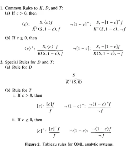
Thus, in addition to the a and /3 rules, Q M L analytic systems contains tableau rules listed in Figure 2.

We can use the classification of wffs to simplify the presentation of the tableau rules as follows:

1. ~r rules

S, #(c)

#(c): (c > O)

K + ( S , 1 - c ) ,

#o(C)

S, #+ (c)

#+(c):

K(S, 1 - c), "rr] (c)

Proof Methods for Reasoning 343 1. Common Rules to K, D, and T:

(a) If c > 0, then (c): S , ( c ) f 7 1 1 - c 1 + : S , ~ [ I - c ] + f K+(S,1 - c ) , f K+(S,1 - c), ~ f (b) If c > O, then (c)+: S , ( c ) + f 711 - c ] : S, -~[1 - c l f K(S,1 - c ) , f K ( S , I - c), ~ f 2. Special Rules for D and T:

(a) Rule for D

K+(S,0) (b) Rule for T i. If c > 0, then [c]:

[clf

-~(1 - c)+: -~(1 -

c)+f

f ~ f ii. If c > O, then [c]+: [ c ] + f ~ ( l - c ) : - ~ ( 1 - c ) f f -~f

Figure 2. Tableau rules for QML analytic systems.

2. v rule for D: 3. v rule for T: S K + (S, 0) v(c): (c > 0)

v(c)

v+(c):

v+(c)

,'0(c) .~ (c)

Now, we have three kind of rules for Q M L tableau method. T h e first ones are the extension rules that include a rules and the v rules for the system T. T h e second ones are the forking rules that include /3 rules. T h e last ones are the modification rules that include rr rules and the v rule for the system D. T h e applicability condition of these rules are same. A rule is applicable to a tableau iff the uncrossed-out nodes in some branch of the

344 Churn Jung Liau and Bertrand I-Peng Lin tableau contains all premises of that rule. However, the effect of these rules are very different. T h e effect of extension and forking rules have been described in the preceding subsection. Let S and C denote the premise and conclusion set of a modification rule respectively. If some branch of a tableau contains S, and let P be the set of all wffs on that branch, then the resultant tableau after applying the modification rule to that branch of the tableau is obtained as follows. First, for each wff in P \ C, add a new copy of the wff to the end of all other branches to which the wff belongs, and cross out all wffs in P \ C on the branch to be modified. Then, the wffs in C \ P is organized as a new branch and attached to the end of the modified branch.

The definition of a derivation is same as that for propositional logic, and a branch is called closed iff it is classically closed or it satisfies one of the following two conditions:

• It contains [1]+f, or ( 1 ) + f . • It contains -1 [0]f, or --1 ( 0 ) f .

Let B be a set of wffs. T h e n the global assumption rule with B is: under any condition, the element of B may be added to the end of any branches of a tableau. Let L = K, D, or T. We say that f is provable with global assumption B in system L by tableau method, written as B ~-/j f , iff there a derivation of a closed tableau from a single node --1 f by tableau rules for L and the global assumption rule with B.

Next, we will construct the correctness and completeness of the tableau methods. But before continuing, let us consider a rule in some details to see why the tableau rules are correct intuitively. Consider the ( c ) + rule. The premises of the rule are S u {(c)+f}, i.e., the wffs in this set are true in some world w. This implies that there exists a world w' such that R(w, w ' ) > c and f is true in w' since by definition, SUpu~w{R(w, u)l u ~M f} > C. However, any wff g in the set K(S, 1 - c) satisfies that [1 - c]g is true in w since by the premises S is true in w. This in turn implies that for any world u such that u ~M -~ g, R(w, u) <_ c. Thus -7 g must be false in w', i.e., g is true in w' for any wff g in K(S, 1 - c). This argument verifies that there exists one world such that the conclusions of the ( c ) + are true in it. However, the problem arises when we consider the ( c ) rule since supu ~ w{R(w, u)lu ~M f} > C does not imply the existence of a world w' such that R(w, w') > c if the set W is infinite. Fortunately, we have Corollary 3.1., which tells us that it is sufficient to consider only finite models.

To construct the soundness result, we need some definitions. Let L = K, D, T, and S be a set of wffs. T h e n S is called finitely L-satisfiable under assumption B iff there exists a finite model M = (W, R, TA) in L such that ~ t B and there exists a world w ~ W such that w WM S. A branch of a tableau is finitely L-satisfiable u n d e r assumption B iff the set of

Proof Methods for Reasoning 345 uncrossed-out wffs on it is. A tableau is finitely L-satisfiable under assumption B iff one branch of it is so. We now have the following lemma. LEMMA 4.1 Let L = K, D, or T. I f T 1 and T 2 are two tableaus and T 2 is the result of applying some tableau rule for L to T 1, then T 2 is finitely L-satisfiable under assumption B if T 1 is, where B is the set with which the global assumption rule is applied.

P r o o f Suppose T 1 is finitely L-satisfiable under B, then there exists one branch of it finitely L-satisfiable under B. If T 2 is obtained from T 1 by applying some tableau rule to any branch except that branch, then obvi- ously, that branch remains satisfiable in the original model, and the result follows. Now, if the rule is exactly applied to that branch, then there are some cases to be considered. Let M = ( W , R, T A ) be a finite L-model such that ~M B and w be a world in W such that the uncrossed-out wffs on the branch are true in it. T h e n

a rules: the new branch extending the original one with a 1 and o/2 is still true in w since a is.

/3 rules: the new branch extending the original one with /31 or that extending with /32 are true in w since /3 is.

7r(c) rules: the set of uncrossed-out wffs on the original branch contains S u {rr(c)}, so by assumption w ~M S U {Tr(c)}. Since W is finite and c > 0, this means there exists one world w' such that w' ~ u 7r0(c) and R ( w , w ' ) > c. This in turn implies w' ~A4 + K+(S, 1 - c) U {Tr0(c)}. Since the uncrossed-out wffs on the modified branch in tableau T 2 are exactly the wffs in this conclusion set, this means tableau T 2 is also finitely L-satisfiable under assumption B. T h e witness is the model M and the new world w'.

~-+(c) rules: the p r o o f is similar as above.

u rule in D: in this case, M is assumed to be a finite serial model. T h e property of seriality and finiteness implies that there exists a world w' in W such that R ( w , w ' ) = 1. This results in w' ~ K+(S,O) since w ~M S. Thus the modified branch in the new tableau T 2 wits the fact that T 2 is finitely D-satisfiable under assumption B.

v(c) rule in T: in this case, M is assumed to be a reflexive model. Since

W [:::::M /](C) and c > 0, then by reflexivity of M, we have w I::::: M lp0(c).

Thus the extended branch in the tbleau T 2 is true in w. v+(c) rule in T: the p r o o f is similar as above.

global assumption rule with B: since the wffs in B are true in all worlds in W, the extended branch wits the finite L-satisfiability of T 2. []

346 Churn Jung Liau and Bertrand I-Peng Lin THEOREM 4.1 (Soundness theorem of tableau method for analytic sys- tems) Let L = K, D, or T, and B be a finite set of wffs, then B H L, f implies B ~L f

Proof If B ~-L' f and B ~:L f , then there exists a finite model M =

(W, R, TA) in L and a world w ~ W such that ~ u B and w ~ u ~ f by

corollary 3.1. This fact results in the initial tableau with a single node -7 f is finitely L-satisfiable under assumption B, then by applying the above lemma repeatedly until the d o s e d tableau is derived. However, it is impossible for a closed tableau to be finitely L-satisfiable under assumption

B, so a contradiction follows. []

We can now turn to the completeness of the analytic systems. Suppose S is a finite set of wffs, then an L-tableau for S under assumption B is any tableau that begins with a single branch consists of all wffs in S and continues by applications of a,/3, ~-, ~, rules for L, and global assumption rule with B. S is called L-consistent under B if no L-tableaus for S are closed.

THEOREM 4.2 (Completeness theorem of tableau method for analytic systems) Let L = K, D, or T, and B be a finite set of wffs. Then B ~L f implies B H L, f"

Proof Define

0 = {SIS c_ Sub(B U {f}), S is L-consistent under B}.

We will show that O is B-compatible L-consistency property by verifying that O satisfies the conditions in Definition 3.2. Let S ~ O, then there are no closed tableaus for S under B. Thus, we have

(a) if a ~ S and S u {al, a 2} ~ ®, then there is a closed tableau for the second set. But we can apply a rule to S first and the resultant tableau is a single branch containing all wffs in S u {aa, a2}- Consequently, there is a closed tableau for S after all, and this is a contradiction.

(b) If /3 ~ S, S t_J {/31} ~ O, and S U {/32} ~i~ ~), then there are closed tableaus for S U {/31} and S U {/32} respectively. Then we can apply /3 rule to the initial tableau for S, and then derive the two closed tableaus for the two branches respectively. Since in our modification rules, the part to be crossed out which is common to other branches is copied to those branches, the derivation of the two branches do not interfere with each other. Thus the final tableau is a closed tableau for S.

(c) if S contains ± , ~ T , ~r+(1), or u+(1), then the initial tableau of S is just a closed tableau for it.

Proof Methods for Reasoning 347 (kl) if c > 0 and 7r(c) e S, then we can apply ~r(c) rule to the initial tableau of S and the resultant tableau is just

K+(S, 1 - c ) u

{Tr0(c)}. Since S has no closed tableau,

K+(S,

1 - c) U {~r(c)} has not, either. Thus,

K+(S,

1 - c) U {~r0(c)} E O.

(k2) the condition is verified analogously.

(d) apply the u rule for D to the initial tableau for S, the resultant tableau is

K+(S,O),

and so

K+(S,O) ~ 0

since S has no closed D-tableau.

(t) if

f ~ K+(S,O),

then f =

Uo(C)(C

> 0) or f = v~(c) for some

u(c)(c

> 0) or v*(c) ~ S, so we can apply the v(c) or

u+(c)

rule for T to attach f to the end of the initial tableau for S. Since S has no closed tableaus, S u {f} ~ O.

Finally, because of the global assumption rule with B, ® is B-compatible. Now, if B ~L, f , then {--1 f} ~ O, so by the model existence theorem,

B ~L f.

[]

5. NATURAL DEDUCTION METHODS

Natural deduction methods are also important proof methods that have been extensively used in classical logic [11]. In general, the natural deduc- tion method is a kind of forward reasoning method in which we deduce conclusions from some assumptions, and then these assumptions are discharged according to some deduction rules. The final form of the conclusion may be a conditional sentence. Thus, the main characteristic feature of natural deduction methods is that we can make assumptions at any point of the deduction process, deduce things from them, and later discharge the assumptions.

According to the description above, the natural deduction system will contain some assumption-discharging rules. Generally, the rules of a natural deduction system may be classified into two kinds. One is the elimination rules in which the conclusions are structurally simpler than the premises because of the elimination of some connectives. The other is the introduction rules in which the conclusions are structurally more complicated than the premises because of the introduction of connectives. The rules to discharge assumptions are in general a kind of introduction rules since discharging some assumptions will make the conclusion more complex to express the assumptions explicitly in the conclusion.

There are different formats to express a natural deduction proof. Here we will choose the one developed by Fitting [4] for modal logic and modify it to meet our need.

First, a deduction is a sequence of wffs in boxes. The first item in a box is an assumption and other wffs in a box are derived according to the rules

348 Churn Jung Liau and Bertrand I-Peng Lin of the natural deduction systems. The boxes may be nested. When a new assumption is introduced, a new box must be created, with that assumption as the first item of the created box. On the other hand, when an assump- tion is discharged by the assumption-discharge rules, a box created for the assumption should be closed off, and the conclusion is written just below the box. A natural deduction proof (abbreviated as proof throughout this section) is a deduction in which all assumptions have been discharged.

Although the boxes may be nested, they should not be overlapped. In other words, a box should be closed off only when all boxes inside it have been closed off. A wff f and a box B are said to be at the same nest level if B and f are inside the same box directly. Here, "directly inside a box B" means "inside B, but not inside any boxes inside B."

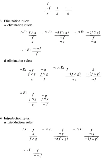
The natural deduction rules for classical logic [4] is presented in Figure 3.

The last line of a proof is the wff that have been proved by the deduction. The global assumption rule with a set of wffs B is that any member of B may be used as a line at any point of the deduction. We write B ~-PL, f to denote that there is a proof of the wrr f with the global assumption B in the classical natural deduction system. Some important properties of classical natural deduction system have been studied exten- sively. We restate some of them from [4] for the sake of reference.

LEMMA 5.1

1. I f B, f ~-PL" g and B, ~ f ~-pL n g, then B ~-PL" g"

2. (Reverse rule) The following assumption-discharging rule holds.

f

[,EMMA 5.2

1. if B, al, ot 2

I"-eL.

f, then B, ot ~-PL" f

2. if B, [31 ~-el~" f and B, [32 ~-eL, f, then B, [3 F-eL, f

Now, we can develop the natural deduction method for the QML analytic systems on the classical deduction basis. We call a deduction or derivation in a box as a subordinate deduction (or just subdeduction). To develop the natural deduction method for the QML systems, we need another kind of box. The original kind of box represents the subdeduction under some assumptions, while the new kind of boxes represent a subde- duction in a possible world. Since our possible worlds are connected by a fuzzy accessibility relation, we must be able to reflect the strength of the

Proof Methods for Reasoning 349 connection between two worlds. We say a word w' is c-accessible (resp. c+-accessible) from the world w iff R ( w , w ' ) > c (resp. R ( w , w ' ) > c).

Thus, we have two types of boxes in the Q M L natural deduction sys- tems. The type 1 boxes are just those of the classical natural deduction system. The type 2 boxes are labeled by c or c ÷ where c ~ [0,1]. Intuitively, the deduction process proceeding in a possible world, while entering a type 2 box labeled with c or c ÷ means to start a deduction in a new possible world that is c-accessible or c+-accessible from the original world. Type 1 boxes and type 2 boxes are distinguished by their labels. If a box has no label, then it is a type 1 box; otherwise, it is a type 2 box.

When we are making deductions in a possible world, we may want to jump to another world to make some deductions. There are at least two ways to do this. The first choice is to make deductions in a generic world that is c-accessible from the present world for some c. When returning from the new world, we get some general results about any worlds that are c-accessible from the present world, and the results are used in the present world to deduce other results. The other choice is to do the same thing in a particular world, and if we can derive some contradiction in the particu- lar world, then the contradiction can be returned to the present world. Thus, two styles of Q M L natural deduction systems are induced. If the former approach is adopted, the obtained system is the so-called A-style natural deduction system. If we follow the latter approach, the resultant system is called I-style system. We will discuss the two styles of systems in the following subsections.

5.1. I-Style Natural Deduction System

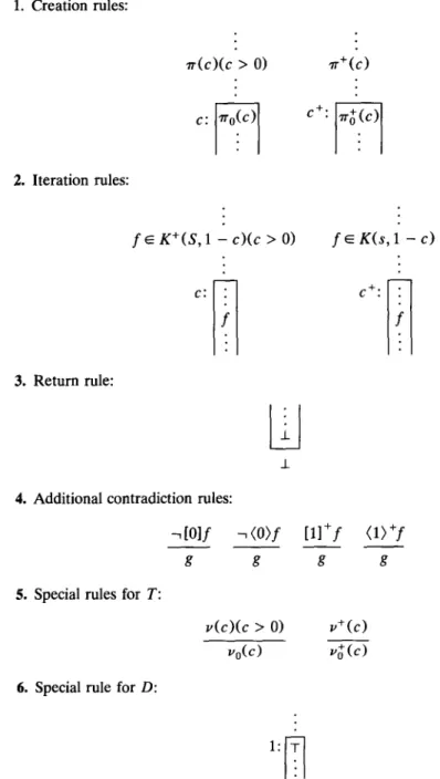
The I-style natural deduction systems for K, D, and T include all inference rules of the classical natural deduction system. However, any rules involving boxes (i.e., the iteration rule and the /3 introduction rules) refer only to the type 1 boxes. Thus, we must develop some rules for type 2 boxes. The following is a complete list of the common rules for 1-style natural deduction K, D, and T systems:

1. Type 2 box creation rule: if a wff 7r(c) (resp. 7r÷(c)) occurs in the course of a deduction, a type 2 box with label c (resp. c ÷) may be created. The created box is at the same nest level as the occurrence of ~ ( c ) (resp. 7r+(c)), and 7r0(c) (resp. ~-~(c)) is put at the first line of the box.

2. Iteration rules for type 2 boxes: If B is a type 2 box with label c (c+), and S is the set of all wffs that occur above B and have the same nest level as B. Then any member of K÷(S, 1 - c)(K(S, 1 - c)) may be repeated directly inside B.

350 Churn Jung Liau and Bertrand I-Peng Lin

1. Iteration rule: in a deduction, if f and box B are at the same nest level and f occurs above B, then f may be repeated directly inside the box B.

2. Contradiction rules: 3. Elimination rules: a elimination rules: AE: f a g f g - n ~ E : f ~ f g J_ -7 T ~ f f fl elimination rules: VE: . ~ f -~g f V g f V g g f g g V E : - ~ ( f v g ) ~ DE: - ~ ( f 3 g ) -~f f ~ g ~ g ~ A E : f g - - ( f A g ) - . ( f A g ) ~ g - ~ f D E : f ~ g f D g f D g g ~ f 4. Introduction rules: a introduction rules: A I : f g f a g -~ v I : _{_~f ~ ~I: f} -~g -~g - ~ ( f V g ) --7(fDg) -.-71: f - 7 - ~ f

Proof Methods for Reasoning

/3 introduction rules (assumption discharging rules):

f v g

f v g

DI: -~ AI: -~(f A g)

f D g

f z g

~ f

Figure

3--Continued

-~(f ^ g) 351

3. Contradiction return rule: if I is derived in a type 2 box, the box may be closed off, and _1_ is returned outside.

4. Contradiction rules: our additional contradiction rules with respec- tively the premises -1 [0If, -1 (0>f, [1] +f, and (1 } +f are included. Furthermore, we have special rules for the system D and T. The special rule for T is directly presented in Figure 4. The special rule for D is as follows: one may create a type 2 box labeled with 1 at any point of the deduction. For convenience, the first line of the so-created box is q-. Schematically, these rules are presented in Figure 4.

The definition of deduction, proof, and global assumption rule is almost same as that for classical logic. However, we require a proof that is a deduction in which all boxes (type 1 or 2) have been closed. We use B ~-L' f to denote that f has a proof in the I-style system for L under the global assumption rule with set B. It is easy to construct the completeness of the I-style systems, so we consider it first.

THEOREM 5.1

Let B be a finite set of wffs and f be a wff. Then B ~L f

implies B ~--L' f

Proof First, let F = S u b ( B U { f } , and O = { S c F I B ~ L ,

ASP_I_}.

We will verify that O is a B-compatible L-consistency property. Then, if B ~L' f, then { ~ f} ~ O. Otherwise, B ~-L' -~ f D _L, and by D E and the reverse rule, we have B ~-L' f after all. Thus, by model existence theorem

B ~ L f .

To verify that 0 is a B-compatible L-consistency property, we go through the following steps. First, the verification of conditions (a) and

352 Churn Jung Liau and Bertrand I-Peng Lin 1. Creation rules: 2. Iteration rules: 3. Return rule: ,r(c)(c > O)

,rr+(c)

C+: ~

f ~ K+(S, 1 - c ) ( c > O) f ~ K ( s , 1 - c)

C+:

4. Additional contradiction rules: -~[0]f

g 5. Special rules for T:

6. Special rule for D:

.1_

~ ( O ) f [ l ] + f (1)+f

g g g

v(c)(c > O) v+(c)

,-'o(C)

~,~-(c)

Proof Methods for Reasoning 353 (b) follows from L e m m a 5.2. Second, condition (c) can be verified by using AE, contradiction, and n I rules.

T o verify condition (kl) and (k2), we present only one case of them, and the other is similar. Assume c > 0 and I t ( c ) ~ S e O, but K÷(S, 1 - c) U {Tr0(c)} ~ ®, then the following is an I-style natural deduction p r o o f of B [--L i A S D 2_. 1. A S ;assumption 2.1r(c) ;1., A E, 7r(c) • S 3.S \ {~-(c)} ;1., A E C; 4.7r0(c) 5.K+ (S, 1 - c ) 6. A K+(S, 1 - c) A 7r0(c) 7. A K+(S, 1 - c ) A 7r0(c) D± 8. L

;2., type 2 box creation ;3., iteration ;4., 5., A I ;K+(S, 1 - c) U {~-0(c)} ~ O ;6., 7., ~ E 9. ± ; ± return I O . A S n ± ; 1 . , 9 . , h i

Note that line 3. of the deduction is a set of wffs, not just a wff. This is a convention to avoid listing all wffs line by line. T h e kind of convention will be used implicitly when writing a natural deduction proof.

If L = D, to verify that condition (d) is satisfied. Suppose that S ~ t9

but K+(S,O) q~ O, then we can find an 1-style p r o o f of B t- v A S n ± as

follows:

1. A S ;assumption 2.S ;1., A E

1: 3.-r ;creation rule for D

4. K + (S, 0) ;2., iteration 5. A K+(S,O) D_I_ ; K + ( S , 0 ) ~ O

6.2_ ; 4 , 5 , D E

7. ± ; _L return 8 . A S p _ I _ ; 1 . , 7 . , h i

If L = T, condition (t) is verified as follows. Let f e K + ( S , 0 ) and S u {f} ~ O. W e will show that B ~-L' A S n 2-. Because f e K+(S, O) implies that f = v~(c) for some c > 0 and v+(c) e S for f = Vo(C) for some c > 0 and v(c) e S. Thus, by special rule for T, f is derivable from S, and then _L is derivable from S. Finally, once again, the result follows by using ~ I rule.

Furthermore, O is B-compatible because of the global assumption rule. []

354 Chum Jung Liau and Bertrand I-Peng Lin The soundness of I-style systems is intuitively obvious. However, to construct the formal result, we need some more definitions.

DEFINnnON 5.1 Given an 1-style deduction for the wff f under the global assumption B. We can define the set of assumptions alive at line n, A(n), for each line of the deduction as follows:

(i) A(O) = 0 .

(ii) if line n is a member of B or comes from a earlier lines by one of the iteration, contradiction, aI, aE, or BE rules, then A(n) =

A(n - 1).

(iii) I f part of the proof looks like

( n ) 5 (n + 1)f2

(re)f3 (m + 1)f4

where (n) represents that the line number is n, then A(n + 1) =

A(n) tO {f2} a n d A ( m + 1) = A(n).

(iv) if part of the proof looks like

(n)f~

c: (c+:) (n + 1)f2

(m)f3 (m + 1)f4

thenA(n + 1) = fDandA(m + 1) = A(n).

Note that in each box of a deduction, there are two kinds of assumptions alive. The first one is that induced by the creation of a type 1 box, and the second one is those imported from the outside. According to the definition above, when we enter a type 1 box, the two kinds of assumptions are both included in the set of alive assumptions. However, when we enter a type 2 box, all assumptions outside it are forgotten. Thus, the alive assumption set in fact depends on the world in which we are doing deduction.