國立交通大學
資訊科學與工程研究所
博 士 論 文
頻率排列碼
On Frequency Permutation Arrays
研 究 生:謝旻錚
指導教授:蔡錫鈞 教授
頻率排列碼
On Frequency Permutation Arrays
研 究 生:謝旻錚
Student : Min-Zheng Shieh
指導教授:蔡錫鈞
Advisor : Shi-Chun Tsai
國立交通大學
資訊科學與工程研究所
博士論文
A DissertationSubmitted to Institute of Computer Science and Engineering College of Computer Science
National Chiao Tung University in partial Fulfillment of the Requirements
for the Degree of Doctor of Philosophy
in
Computer Science and Engineering June 2010
Hsinchu, Taiwan, Republic of China
�
�
令n為正整數m與λ的乘積。一個長度為n、最小距離為d的頻率排列碼(frequency permu-tation array,簡稱FPA)是一個包含若干個由m個符號各重複出現λ次所形成的排列,並且 其中相異的兩個排列的距離至少為d。FPA是排列碼(permutation array,簡稱PA)的一般 化,PA即是FPA取λ = 1時的特例。目前PA已有許多領域的應用,諸如電力線通訊、快閃 記憶體資料儲存以及密碼學。FPA具有比PA更大的設計彈性,因此在各方面應用上均有較 PA更高的潛力。 在本篇論文中,吾人透過估計特定半徑內的頻率排列個數,證明了在柴比雪夫距離 (Chebyshev distance)下,FPA元素數量之Sphere-packing類型上界以及Gilbert-Varshamov類 型下界。此外,吾人亦提出兩個有效率的演算法,用以正確計算出特定半徑內的頻率排列 個數。其中之一能在O((2dλ dλ )2.376 log n)的時間複雜度以及O((2dλ dλ )2) 的空間複雜度完成計 算。另外一個則僅需O((2dλ dλ )(dλ+λ λ )n λ ) 的時間與O((2dλ dλ )) 的空間資源便能完成。當λ與d均為 常數時,這兩個演算法均能有效率的求出特定半徑內的頻率排列個數。 吾人發明數個建造FPA的方法,並藉由此推導出對應的FPA元素數量下界。這些建造的 方法中,有些類型的FPA具有高效率的編碼與解碼方式,而其中一個更具有區域可解碼演 算法以及列表可解碼演算法。吾人展示了如何在僅讀取λ + 1個符號的情況下,解出一個資 訊符號,以及針對一個任意給定的排列,如何找出所有特定距離內FPA中的元素。此外, 藉由區域可解碼演算法,吾人亦造出一個私密資料取回的安全協定。 吾人透過研究子群碼(subgroup code)的性質,證明了在一般情況下,計算出任一FPA的 最小距離是困難的。子群碼是PA的一個特例,其中任兩個元素,在函數合成的運算下, 具有封閉性。吾人證明,在柴比雪夫距離下,計算子群碼的最小距離,等價於計算其中非 (non-identity permutation)之最小權重。更進一步的,吾人證明了後者係為一NP-complete問 題,以及對任一常數ϵ,逼近子群碼之最小距離至2− ϵ的倍率,亦為NP-hard。Abstract
Let m and λ be positive integers. A frequency permutation array (FPA) of length n = mλ and distance d is a set of permutations on a multiset over m symbols, where each symbol appears exactly λ times and the distance between any two elements in the array is at least d. FPA generalizes the notion of permutation array (PA), which is a special case of FPA by choosing λ = 1. PAs are known for various applications in power line communication, flash memories and cryptography. FPAs are more flexible than PAs, since the length and the symbol set size of a PA must be equal. FPAs are potentially better than PAs in various of applications. For example, FPAs have higher information rate than PAs do when their symbol sets are the same.
In this thesis, under Chebysheve distance, we prove a Gilbert-Varshamov type lower bound and a sphere-packing type upper bound on the cardinality of FPA via bounding the size of balls of certain radii. Moreover, we propose two efficient algorithms that compute the ball size under Chebyshev distance. The first one runs in O((2dλ
dλ )2.376
log n) time and O((2dλ
dλ )2)
space. The second one runs in O((2dλ
dλ )(dλ+λ λ )n λ ) time and O((2dλ dλ )) space. For small constants λ and d, both are efficient in time and use constant storage space.
We give several constructions of FPAs, and we also derive lower bounds from these con-structions. Some types of our FPAs come with efficient encoding and decoding capabilities. In addition, we show one of our designs is locally decodable and list decodable. In other words, we illustrate how to decode a message bit by reading at most λ + 1 symbols, and how to find the list of all codewords within a certain distance. Furthermore, we propose an FPA-based private information retrieval scheme, which follows from the locally decodable property.
On the other hand, we show that it is hard in general to determine the minimum distance of an arbitrary FPA by investigating subgroup codes. Subgroup permutation codes are per-mutation arrays exhibiting group algebra structures with the composition operator. Under Chebyshev distance, we prove that to determine the minimum distance of a subgroup code is equivalent to finding the minimum weight of non-identity codewords in a subgroup permu-tation code. Moreover, we prove the latter is NP-complete and it is NP-hard to approximate the minimum distance of a subgroup code within the factor 2− ϵ for any constant ϵ > 0.
Acknowledgments
I would like to thank my parents for giving me a chance to accomplish this thesis. I am greatly indebted to Dr. Shi-Chun Tsai, my advisor, for guiding and encouraging me. I also wish to thank Dr. Wen-Guey Tzeng, Dr. Hsin-Lung Wu, Dr. Chia-Jung Lee, Mr. Ming Yu-Hsieh, Mr. Ying-Jie Liao, Mr. Te-Tsung Lin, Mr. Chang-Chun Lu, Mr. Jynn-Jy Lin, Mr. Min-Chuan Yang, Mr. Li-Rui Chen and all the other members in the CCIS research group for sharing their wisdom with me.
Contents
1 Introduction 1
1.1 Permutation Arrays and Their Applcations . . . 1
1.2 Frequency Permutation Arrays . . . 4
1.3 Our Results . . . 5
1.4 Organization of the Thesis . . . 6
2 Preliminaries 7 2.1 Notations . . . 7
2.2 Coding Theory . . . 11
2.3 Computational Complexity . . . 13
3 Explicit Lower and Upper Bounds 17 3.1 Gilbert Type and Sphere Packing Bounds . . . 17
3.2 Enumerate Permutations in a Ball . . . 22
3.3 Compute the Ball Size . . . 27
4 Constructions and Related Bounds 33 4.1 An Explicit Construction . . . 33
4.2 Recursive Constructions . . . 34
5 Codes with Efficient Encoding and Decoding 41 5.1 Encoding Algorithm . . . 41
5.2 Unique Decoding Algorithm . . . 43
5.4 List Decoding Algorithm . . . 46
5.5 Private Information Retrieval . . . 48
6 Complexity Issues 51 6.1 Complexity Problems Related to FPAs . . . 51
6.2 Minimum Distance of Subgroup Codes . . . 53
6.3 Cameron-Wu’s Reduction . . . 68
7 Conclusion and Future Works 71 7.1 Conclusion . . . 71
7.2 Future Works . . . 71
7.3 Code-Anticode Type Bounds . . . 73
7.4 Steganography . . . 73
7.5 Covering Radius . . . 74
A Tables of Ball Size 83 B Program Codes 93 B.1 Computing the Ball Size in Python 3 . . . 93
List of Tables
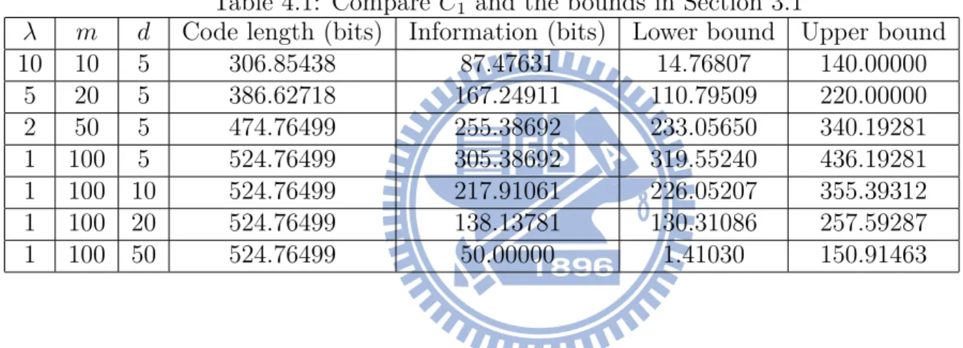
4.1 Compare C1 and the bounds in Section ?? . . . . 34
6.1 Weight contribution of different gadgets . . . 57
6.2 Operation of Klein four-group. . . 58
6.3 Operation of basic construction blocks and their products. . . 60
6.4 Weights of the basic construction blocks . . . 60
6.5 Weights of modified basic blocks . . . 61
A.1 The table of ball size under ℓ∞-metric for λ = 2, m∈ [20], d = 2 . . . . 84
A.2 The table of ball size under ℓ∞-metric for λ = 2, m∈ [20], d = 3 . . . . 85
A.3 The table of ball size under ℓ∞-metric for λ = 2, m∈ [20], d = 4 . . . . 86
A.4 The table of ball size under ℓ∞-metric for λ = 2, m∈ [20], d = 5 . . . . 87
A.5 The table of ball size under ℓ∞-metric for λ = 3, m∈ [20], d = 2 . . . . 88
A.6 The table of ball size under ℓ∞-metric for λ = 3, m∈ [20], d = 3 . . . . 89
A.7 The table of ball size under ℓ∞-metric for λ = 4, m∈ [20], d = 2 . . . . 90
List of Figures
3.1 EnumVλ,n,d(k, P ) . . . . 23
3.2 Graph G2,6,1 . . . 28
3.3 Graph H2,1 . . . 29
4.1 The extension algorithm ϕk(y, x) . . . . 35
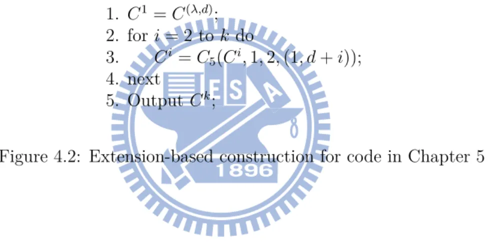
4.2 Extension-based construction for code in Chapter ?? . . . . 39
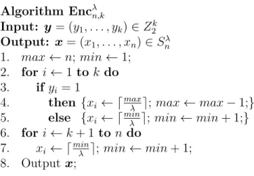
5.1 Encλ n,k encodes messages in Z2k with Snλ. . . 42
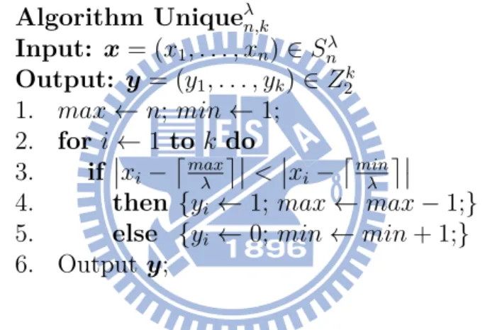
5.2 Uniqueλ n,k decodes words in Snλ to messages in Z2k. . . 43
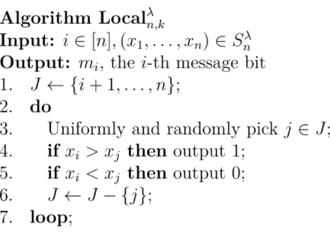
5.3 Localλ n,k decodes one bit by reading at most λ + 1 symbols. . . . 45
5.4 Listλ n,k gives a list of candidates of the closest codewords. . . 47
6.1 The sketch of reduction . . . 54
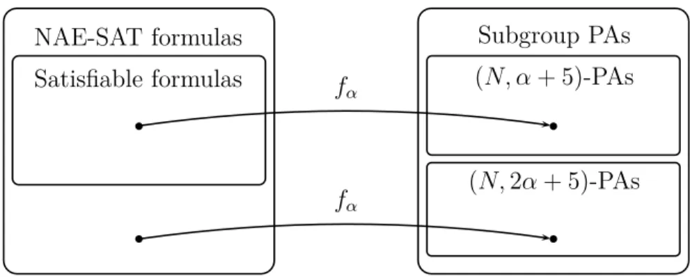
6.2 Satisfiable ϕ is mapped into (N, α + 5)-PA f (ϕ). . . . 55
6.3 Unsatisfiable ϕ′ is mapped into (N, 2α + 5)-PA f (ϕ′). . . 56
6.4 No position is permuted by 2 kinds of gadgets. . . 56
6.5 κ′1χ = χκ′1 . . . 59
Chapter 1
Introduction
Let Sλ
n be the set of all permutations on the multiset { λ z }| { 1, . . . , 1, . . . , λ z }| { m, . . . , m}. A frequency permutation array (FPA) is a subset of Sλ
n for some positive integers m, λ and n = mλ. In this thesis, we investigate their properties and applications. In addition, we study how to construct FPAs with efficient encoding and decoding algorithms. On the other hand, we analyze the complexity of computational problems related to FPAs.
1.1 Permutation Arrays and Their Applcations
A permutation array (PA) is simply a special case of an FPA by choosing λ = 1. PAs have been studied for a long time. Based on Slepian’s [36] idea, the first error correcting PA is proposed by Blake [5] in 1974. Today, PAs have applications in various fields. Recently, researchers have found that PAs have applications in areas such as power line communication (e.g. [31], [41], [42], and [43]), block cipher (see [13]) and multi-level flash memories (see [20], [21] and [37]).
The communication devices will not work without electricity, so most of them are sup-posed to have a power line connected. As a consequence, power lines are considered as a highly potential solution for the last-mile connection. Vinck and Häring [41] proposed a transmission scheme using 4-Frequency-Shift-Keying (4-FSK) modulation coded by permu-tation arrays over the power lines. When transmitting data with m-FSK modulation, we send symbol i∈ {1, . . . , m} by a carrier wave of some unique frequency fi. For example, we
send (1, 3, 2, 4) by setting the frequency of the carrier wave to f1, f3, f2 and f4 in time slot
1, 2, 3 and 4, respectively. After the carrier wave passes through a noisy channel, the receiver may get extra symbols in some time slots. If there is a noise wave of frequency f4 happening
in time slot 1, then the receiver would get{f1, f4} in time slot 1. There are two major noises
in the channel over power lines,
1. Narrow band permanent noise. This kind of noise is generated by certain electronic devices such as television and computers. It often appears in every time slot. Thus, we alway receive symbol i when a device generate a narrow band permanent noise of frequency fi. The receiver may get{f1, f2}, {f2, f3}, {f2} and {f2, f4} in time slot 1, 2, 3
and 4, respectively, if there is a permanent noise of frequency f2.
2. Broad band impulse noise. An impulse noise can be caused by unplug a heavy load device or a power surge. It makes us to receive all symbols in a time slot. The receiver may get {f1}, {f3}, {f2} and {f1, f2, f3, f4} in time slot 1, 2, 3 and 4, respectively, if
there is an impulse noise of frequency in time slot 4.
The structure of permutation is robust against these noises, since every symbol appears exactly once in a permutation. For the narrow band permanent noise, we can find out the extra symbol, because the extra symbols are identical in every time slot. A permutation on {1, . . . , n} can be uniquely determined if we know the symbols in n − 1 entries of it. Consequently, we can indicate the correct symbol in the time slot where the impulse noise happens. With error correcting capability, PAs can overcome others minor noises to ensure the communication quality over power lines.
Flash memory has become one of the most important type of non-volatile data storage recently. The basic unit of a flash memory is a cell, which behaves like a battery. A multi-level flash memory cell can store m kinds of symbols where m > 2. The stored symbol is quantized by the discrete levels v0, v1, . . . , vm of the cell voltage. For example, a cell represents symbol i if its voltage ranges from vi−1 to vi. One of the noticeable property of flash memory is the asymmetry of charging and discharging cells. It is possible to put electrons only into one cell in a short time, but removing electrons from a cell is not allowed. We can only relatively slowly remove all electrons in a block, which consists of about 105 cells (see [8]). This causes
some problems on data writing.
1. Even when we want to only write one cell, we need to erase a block, i.e., to remove all charges in it, then perform charging on each cell in it. This makes writing data into a cell slow. Moreover, the life time of a flash cell is heavily related to the number of discharges performed.
2. The overshooting problem. It is hard to accurately control the amount of electrons charged into a cell. There are often two charging strategies. The first one is to charge a large amount to the cell. If lucky, then we can write the cell correctly in one charge. Otherwise, we have to discharge the whole block slowly, and we need to charge every cell in the block. The second one is to charge a small amount to the cell, then check whether the voltage is high enough to represent the symbol. We might need to repeat for several times to accomplish the writing.
In order to accelerate the writing, Jiang et al. [20] illustrate the rank modulation for multi-level flash memory. Instead of symbol quantization with voltage multi-levels, their concept is to represent symbols in accordance with the ranking of relative voltage levels. Therefore, we can change the symbol usually by several charging operations, and the frequency of discharging the block decreases significantly. Moreover, when the overshooting problem occurs, it can be fixed by several charging operation in general. Since the expected number of discharg-ing decreases, the rank modulation scheme increases both the writdischarg-ing performance and the endurance of the multi-level flash memory. Furthermore, Jiang et al. [21] proposed some error correcting codes, which are exactly PAs, for storing data in multi-level flash memory. The overshooting problem can be solved directly by the error correcting scheme. The error correcting capability of PAs also provides immunity from the other problems.
In the past decade, many constructions have been proposed. These methods include ap-plying distance preserving mapping (DPM) (see [9]), and distance increasing mapping (DIM) to linear block codes (e.g. [10] and [11]), exploiting the connection between PAs and mutually orthogonal latin squares (MOLS) [12], and the others (e.g. [26] and [37]). Conversely, re-searchers also studied the maximum cardinality of PAs under various settings. For instances, Deza and Vanstone [14] gave bounds on the maximum cardinalities of equidistant PAs
un-der Hamming distance, and recently, Kløve et al. [26] proposed bounds unun-der Chebyshev distance.
There are plenty of choices for constructions of PAs, however, only few families of PAs known to have both efficient (in polynomial time of the codeword length) encoding and decod-ing algorithms, such as the codes proposed by Lin et al. [28] and by Swart and Ferreira [35]. Some constructions, such as Babaev’s [3], consider encoding as computing the binary rep-resentation for some permutation, and decoding as computing the permutation represented by some binary string. The schemes in [3] are efficient, but they do not exhibit any error correcting capability. Swart and Ferreira [35] gave a decoding algorithm for a particular PA applied to power line communication. Lin et al. [28] proposed a couple of novel constructions with efficient encoding and decoding algorithms for PAs under Chebyshev distance.
1.2
Frequency Permutation Arrays
FPA was proposed by Huczynska and Mullen [17] as a generalization of PA. They gave several constructions of FPA under Hamming distance and bounds on the maximum array size. Some of their constructions extend the concept of MOLS. They also gave bounds on the maximum cardinality of FPAs under Hamming distance.
Similar to the application of PAs for power line communication, we can encode a message as a frequency permutation from Sλ
n. Then the message is transmitted as m-FSK signals. The nature of frequency permutations provides higher information rate without losing immunity to narrow band permanent frequency disturbances and broad band impulse noise mentioned in Vinck’s work [43], since the numbers of different symbols are equal.
For flash memory applications, different from the approach by Jiang et al. [21], we can use FPA to provide multi-level flash memory with error correcting capabilities. For example, suppose a multi-level flash memory, where each cell has m states, which can be changed by injecting or removing charge into or from it. Over injecting or charge leakage will alter the state as well. We can use the charge ranks of n cells to represent a frequency permutation from Sλ
n, i.e., the cells with the lowest λ charge levels represent symbol 1, and so on.
more severe failure in data storage. However, the lengths of PAs are limited by the size of their symbol set, which can be the number of distinct frequencies of power line or the number of charge levels of flash memory. For FPAs, there is no such limitation. We can easily construct much longer FPAs, especially, the codeword length of an FPA can be as long as the block length of a multi-flash memory. Hence, FPAs are more suitable for these applications.
1.3 Our Results
First of all, we prove a Gilbert-Varshamov type lower bound and a sphere-packing type upper for the maximum cardinality of FPAs under Chebyshev distance. We obtain the close form by estimating the size of ball by bounding the permanent of a special family of matrices. We also give several efficient dynamic programming style algorithms to compute the exact ball size by investigating an enumeration algorithm closely.
Then, we give several methods to construct FPAs under Chebyshev distance. These meth-ods include a direct construction and various recursive constructions. They mainly extend the ideas from the work of Kløve et al. [26]. We give efficient encoding and decoding algo-rithms for a family of FPAs. The decoding algoalgo-rithms include a unique decoding algorithm, a local decoding algorithm and a list decoding algorithm. Therefore, FPAs exhibit strong capabilities in error correcting.
A locally decodable code has an extremely efficient decoding for any message bit by reading at most a fixed number of symbols from the received word. Suppose that an FPA is applied to a multi-level flash memory where the length of a codeword equals the block length. This feature allows us to retrieve the desired message bits from a multi-level flash without accessing the whole block. With the locally decodable property, we can raise the robustness of the code without loss of efficiency. Also, we show our construction of FPA can be used in cryptographic application. Locally decodable codes have been under study for years, see [38] for a survey and [45], [16] for recent progress. They are related to a cryptographic protocol called private information retrieval (PIR for short).
distance of a code hard?” and “How fast can we compute the closest codeword for a certain received string?” may be the top two problems frequently asked. For λ = 1, both problems are proved to be NP-complete under many metrics, such as Hamming distance, Chebyshev distance (ℓ∞-metric), Kendall’s tau, et al.[7, 6]. However, for Chebyshev distance, the NP-completeness proof by Cameron and Wu [7] fell apart on some instances. We give a correct proof for the NP-completeness. Moreover, we also show the problem is NP-hard to approxi-mate within 2− ϵ for every constant ϵ > 0.
1.4
Organization of the Thesis
In Chapter 2, we will give notations used throughout this thesis and some background knowl-edge of permutations, computational complexity and coding theory. In Chapter 3, we present how to obtain explicit bounds on the maximum cardinality of FPAs. In Chapter 4, we give both explicit and recursive methods to construct FPAs of certain parameters. In Chapter 5, we show an efficient encoding and three decoding algorithms for a family of FPAs con-structed in a simple manner. In addition, we construct a protocol for private information retrieval based on the locally decodable property. In Chapter 6, we discuss issues in the aspect of computational complexity. Finally, we conclude this thesis with some future works in Chapter 7.
Chapter 2
Preliminaries
2.1 Notations
Here, we give useful notations. Let (a1, a2, . . . , an) denote an n-tuple. We use [n] to represent the set {1, . . . , n} and [n1, n2] to denote the set {n1, n1 + 1, . . . , n2} where n1 < n2. A
permutation on [n] is a bijective function from [n] to [n]. In this thesis, we use n-tuples to denote functions and permutations.
Definition 2.1.1. (n-tuples) A function f = (a1, a2, . . . , an) if and only if f (i) = ai for every i∈ [n].
Let Sn denote the set of all permutations on [n]. Sn is a group with the composition operation, since the composition of two bijective functions from [n] to [n] is still a bijective function from [n] to [n]. We define the product of two permutations f and g∈ Sn as
f g = (f (g(1)), . . . , f (g(n))) .
The identity in Sn is en = (1, . . . , n). fm represents the m-th power of a permutation f on [n], and we define f0 = en and fm = f fm−1 for m > 0. A permutation f of order k on [n] if and only if k is the minimum positive integer such that fk= e
n. We say that {g1, . . . , gk}
is a generator set for a subgroup G ⊆ Sn, if every permutation g ∈ G can be written as a product of a sequence of compositions from elements in the generator set.
To represent a permutation, there is an alternative other than using an n-tuple. We can write a permutation as a product of cycles. A cycle (a1, a2, . . . , ap) represents a permutation π such that
• π(ap) = a1.
• π(ai) = ai+1 for i∈ [p − 1].
• π(x) = x for x /∈ {ai : i ∈ [p]}. We say two cycles (a1, . . . , ap) and (b1, . . . , bq) are disjoint if {a1, . . . , ap} ∩ {b1, . . . , bq} = ∅. Every permutation π ∈ Sn can be written as
a product of disjoint cycles.
Definition 2.1.2. (Products of cycles) For 0 = p0 < p1 < · · · < pq < pq+1 = n and {a1, . . . , an} = [n], a permutation π = (a1, . . . , ap1)(ap1+1, . . . , ap2)· · · ( apq+1, . . . , an ) if and only if π(ai) = ai+1 , i /∈ {p1, . . . , pq+1}. apj−1+1 , i∈ {p1, . . . , pq+1} and i = pj.
For example, (3, 2, 1, 5, 6, 4, 7) = (1, 3)(2)(4, 5, 6)(7). For simplicity, we sometimes omit the cycles of one element, i.e., (1, 3)(2)(4, 5, 6)(7) = (1, 3)(4, 5, 6). When written in the product of cycles notation, the structure of a permutation is clearer. Now, we show how to relabel a permutation without changing its structure.
Lemma 2.1.3. For permutations f and g = (a1, . . . , ap1)(ap1+1, . . . , ap2)· · ·
(
apq+1, . . . , an ) on [n], we have
f gf−1 = (f (a1), . . . , f (ap1))(f (ap1+1, . . . , f (ap2))
(
f (apq+1), . . . , f (an) )
Proof. We rewrite g as
(a1, g(a1), . . . , gp1−1(a1))(ap1+1, g(ap1+1), . . . , g
p2−p1−1(a p1+1))· · · ( apq+1, . . . , g n−pq−1(a pq+1) )
Consider the sequence f (a1), f gf−1(f (a1)), (f gf−1)2(f (a1)), . . . , (f gf−1)p1(f (a1)), they are
actually
f (a1), f (g(a1)), f (g2(a1)), . . . , f (gp1−1(a1)), f (a1),
since (f gf−1)k = f gkf−1 and gp1(a
1) = a1. Therefore, the cycle structure of a1, . . . , ap1 in g
and the cycle structure of f (a1), . . . , f (ap1) in f gf−1 are the same. Apply this observation
to f (ap1+1), . . . , f (apq+1), then we know the lemma is true.
Here, we give a definition to metric functions. A function δ(·, ·) : D × D → R is a metric function if
• δ(x, y)≥ 0 for every x, y ∈ D. • δ(x, y) = 0 if and only if x = y. • δ(x, y) = δ(y, x) for every x, y∈ D.
• δ(x, y)≤ δ(x, z) + δ(z, y) for every x, y, z ∈ D.
For convenience, when a bold-type alphabet represents an n-tuple, the same alphabet in regular-type with subscript i represents the i-th entry of the n-tuple unless stated otherwise. For example, x = (x1, . . . , xn). For two n-tuples x and y, some well known metrics are defined as follows.
Definition 2.1.4. Hamming distance between x and y is defined as
dH(x, y) =|{i ∈ [n] : xi ̸= yi}|.
Definition 2.1.5. Minkowski distance of order p > 0 between x and y is defined as
ℓp(x, y) = p √∑ i∈[n]|xi− yi| p .
Definition 2.1.6. Chevyshev distance between x and y is defined as
ℓ∞(x, y) = max
The distance between two permutations is the distance between the tuples representing them. We say two permutation (tuples) x and y are d-close to each other under metric δ if δ(x, y) ≤ d. A metric δ is right-invariant if and only if δ(xz, yz) = δ(x, y) for all permutations x, y and z. We show that Hamming distance, Minkowski distance of order p > 0 and Chebyshev distance are right-invariant.
Lemma 2.1.7. For n-tuples x, y and a permutation z ∈ Sn, we have dH(xz, yz) = dH(x, y), ℓp(xz, yz) = ℓp(x, y) and ℓ∞(xz, yz) = ℓ∞(x, y).
Proof. By the definitions, we have
dH(xz, yz) = {i∈ [n] : xz(i)̸= yz(i)}
= |{j : xj ̸= yj for some i∈ [n] with j = z(i)}| = |{i ∈ [n] : xi ̸= yi}| = dH(x, y), ℓp(xz, yz) = p √∑ i∈[n] xz(i)− yz(i) p = √∑p i∈[n]|xi− yi| p = ℓp(x, y), and ℓ∞(xz, yz) = max i∈[n] xz(i)− yz(i) = max i∈[n] |xi− yi| = ℓ∞(x, y).
We define the weight function wtδ(x) for a right-invariant metric δ and a k-tuple x as wtδ(x) = δ(ek, x). For any right invariant metric δ, the distance between the closest pairs of elements in a subgroup G of Sn is equal to the minimum weight of non-identity permutation
in G, since
min
x,y∈G,x̸=yδ(x, y) =x,ymin∈G,x̸=yδ(xy
−1, e
n) = min
x∈G,x̸=en
wtδ(x).
Now, we extend the definition of permutations. A permutation on a multiset{a1, a2, . . . , ak}
is a k-tuple (af (1), af (2), . . . , af (k) )
where f is a bijective function from [k] to [k]. In 1965, Slepian [36] considered a code of length n for permutation modulation. It consists of all multiple permutations on the multiset
{ λ1 z }| { µ1, . . . , µ1, . . . , λm z }| { µm, . . . , µm}
where µ1 < µ2 <· · · < µm and λ1 + λ2+· · · + λm = n. Here, we consider a special case of
Slepian’s code. Let n, m and λ be positive integers where n = mλ. Let Sλ
n be the Slepian’s code where µ1 = 1, µ2 = 2, . . . , µm = m and λ1 = λ2 = · · · = λm = λ. In other words, Snλ is the set of all multiple permutations on {
λ z }| { 1, . . . , 1, . . . , λ z }| { m, . . . , m}. In particular, Sn = S1 n. Every element in Sλ
n is called a frequency permutation of length n and frequency λ. The identity frequency permutation eλ
n in Snλ is (1, . . . , 1, . . . , m, . . . , m).
2.2 Coding Theory
Codes are one of the most important objects which have been studied for decades in both computer science and communication engineering, since they have many applications in the-oretical fields and practical uses. These applications of codes include error-detection and error-correction in communication, data storage, data compression, cryptography, computa-tional complexity theory, etc. In this section, we give a brief but necessary introduction to coding theory. A code C is a set of sequences over a certain symbol set. An element in a code is called a codeword which represents a particular message. An encoding algorithm for code C computes the corresponding codeword in C for any message. A decoding algorithm, which is basically the inverse function of an encoding algorithm, recovers the message from a codeword or even from a corrupted one.
We say a code C is a block code if every codeword in C has the same length. One of the most important parameters of block codes is the minimum distance. The distance between
two codewords can be measured by a certain metric function δ. In different applications or en-vironments, we may choose different metric functions, such as Hamming distance, Minkowski distance, Chebyshev distance, Kendall’s tau distance, and etc. The minimum distance dδ(C) of a block code C under some metric δ is defined as the minimum distance between distinct codewords x and y in C, i.e.,
dδ(C) = min
x,y∈Cδ(x, y).
It is well known that the error-detection capability and the error-correction capability of a code heavily depend on its minimum distance.
Theorem 2.2.1. (Error detection) 0 < δ(c, x) < dδ(C) implies x /∈ C, for any block code C of length n, any codeword c∈ C and any n-tuple x.
Proof. By way of contradiction, assume x is a codeword. Then, we have
dδ(C)≤ δ(c, x) < dδ(C),
a contradiction.
Theorem 2.2.2. (Error correction) Given a block code C of length n, a codeword c∈ C and
an n-tuple x. If δ(c, x) < dδ(C)
2 , then c is the codeword closest to x.
Proof. By way of contradiction, assume c′ ̸= c is the closest codeword to x. Since δ(·, ·) is a metric and δ(x, c′) < δ(c, x) < dδ(C)
2 , we have
dδ(C)≤ δ(c, c′)≤ δ(c, x) + δ(x, c′) < dδ(C),
a contradiction.
Therefore, a block code is considered as a more powerful error detecting code or a error correcting code when it has larger minimum distance.
Another important parameter of codes is information rate. Codes of higher information rate have less space redundancy. The information rate of a block code is the ratio of its message length to its codeword length. The length of a block code C is the average number
of bits to represent a codeword. The message length is log2|C|, i.e., the number of bits sufficient to represent a message. In general, codes of larger minimum distance have lower information rate.
One can find the code of largest minimum distance under constraints on the information rate by enumerating all possible candidates. Although this code is the most powerful one against errors among all codes of the same information rate, it does not mean that this code is suitable in practical use. One of the reasons is that we probably do not have the computation power to enumerate every possible codes under such constraints. In other words, the best one does exist, but we may not know what it explicitly is. Another reason is that we probably do not know any efficient encoding and decoding algorithms for this code. Therefore, we need systematic methods to constructing codes for certain codeword lengths, information rates and minimum distances. Moreover, we need codes with efficient encoding and decoding algorithms. In this thesis, we propose several construction to generate codes with predetermined information rate and minimum distance. Some of them have efficient encoding and decoding algorithms.
A (λ, n, d, δ)-FPA C is a subset of Sλ
n and the minimum distance of C under δ. The codeword length of an FPA C ⊆ Sλ
n is log2|Sn| bits. The message length of an FPA C isλ
log2|C|, where |C| is the cardinality of C. Therefore, the information rate of C is log2|C|
log2|Sλ n|. For a fixed length n, an FPA C has a smaller symbol set when it has a higher frequency. Thus, FPAs of frequency more than 1 have a higher information rate than PAs of the same length. This is one of the reasons why FPAs can replace PAs in various applications.
2.3 Computational Complexity
In this section, we give some background knowledge about computational complexity theory. There are two main categories of computational problems. The first kind is the decision problems. The answer to a decision problem is either ‘yes’ or ‘no’. For example, “Given a real number r, a block code C and a metric δ, is the minimum distance of C under δ less than r?” is a decision problem. The second kind is the optimization problems. In order to define an optimization problem, we need
• An instance set X.
• The set of feasible solutions f (x) for every instance x∈ X.
• A cost function c(·, ·), which maps (x, y) into a real number where x ∈ X and y ∈ f(x). • A goal, which is either minimization or maximization.
The answer to an optimization problem on an instance x can be the best feasible solution y ∈ f(x) or the value of c(x, y), depending on the description of the problem. For example, “Given a block code C and a metric δ, find the minimum distance of C under δ.” Each feasible solution for this problem consists of two distinct codewords y1 and y2. The cost function is
δ(y1, y2), the goal of this problem is minimization. In this case, the answer is a number
representing the minimum distance of C under δ. There is another version of this problem: “Given a block code C and a metric δ, find the closest pair of distinct codewords in C under δ.” The answer to this version is the feasible solution with the smallest cost. Every optimization problem has a corresponding decision problem which is to ask if a feasible solution of certain cost exists. In this thesis, we discuss both decision problems and optimization problems related to FPAs in Chapter 6.
The complexity of an algorithm is measured by how much resource, including time and space, is consumed. It is often a function of the size of the input of the algorithm. The input size of a problem instance is the length of its description. E.g., the input size of an instance of the problem, “Given a block code C of length k, find the minimum distance of C under the ℓ∞-metric”, is k|C|, since each codeword in C has length k. An algorithm is considered to be more efficient if it has lower complexity. In general, we say an algorithm is time efficient if and only if its time complexity is bounded by a polynomial in terms of its input size, or just simply say, it runs in polynomial time. In Chapter 5, we consider the input size of the encoding and the decoding algorithms as the lengths of message and received frequency permutations, respectively. Therefore, checking all possible codewords is not efficient, since |C| can be an exponential function of the intput length.
The complexity of a problem is defined by the complexity of algorithms solving it. Besides providing an explicit algorithm for a problem, we can also use reduction to obtain complexity results on problems.
Definition 2.3.1. A decision problem A is polynomial-time reducible to another decision
problem B, denoted as A≤p B, if there is a polynomial-time computable function f such that 1. f maps instances in A into instances in B.
2. The answer to an instance x in A is ‘yes’ if and only if the answer to the corresponding instance f (x) in B is also ‘yes’.
A≤p B means A is not harder than B when polynomial-time algorithms are considerably efficient. If there is an efficient algorithm (in polynomial time) for B, then we can solve instance x in A efficiently by
1. Compute f (x) in polynomial time.
2. Run the efficient algorithm for B on input f (x). 3. Output the result of the algorithm.
Now, we define the following two best known complexity classes P and NP.
Definition 2.3.2. We say a problem A is in P if there is a deterministic algorithm which
always output the answer for every instance of it in polynomial time.
Definition 2.3.3. We say a problem A is in NP if there is a polynomial time verifier v such
that
• It takes an instance in A and a witness as input.
• For every ‘yes’-instance x, there is a witness w such that v(x, w) accepts. • For every ‘no’-instance x′ and every witness w′, v(x′, w′) always rejects.
The problems in P are the problems which can be solved efficiently by polynomial-time algorithms, and every ‘yes’-instance of problems in NP can be efficiently verified with some witness. The P versus NP problem is asking whether P and NP are the same, in other words, are the problems in NP as easy as those in P? This problem remains unsolved today, and many researchers believe P ̸= NP. Recall that algorithms not in polynomial time are considered as inefficient algorithms. We define the best-known classes representing hard problems as follows.
Definition 2.3.4. We say a problem A is NP-hard if every problem B ∈ NP, B ≤p A.
Definition 2.3.5. We say a problem A is NP-complete if A is in NP and A is NP-hard.
According to the concept of reduction, NP-hard problems are not easier than every NP problem. If an NP-hard problem can be solved in polynomial time, then every NP problem can be solved in polynomial time. Hence, we consider N P -hard problems cannot be solved efficiently unless P = NP. Moreover, NP-complete problems are the hardest problems in NP. The optimization problem is generally harder than its decision version. Consequently, an optimization problem is NP-hard if its decision version is NP-hard. Unless P = NP, we cannot find the optimal solutions for NP-hard optimization problems in polynomial time. So we often seek approximation algorithms for them. We say that an algorithm A is an r-approximate algorithm for a minimization problem (or for a maximization problem) if A always outputs a feasible solution whose cost is no more than r times (no less than 1
r times) of the minimum (maximum) cost on any input. Note that A cannot output an answer whose cost is less (larger) than the minimum (maximum) cost for minimization (maximization) problems, since it is not a feasible solution. Unfortunately, some problems do not allow polynomial time r-approximate algorithm for some r, unless P = NP. We call this kind of complexity results as inapproximable results.
Chapter 3
Explicit Lower and Upper Bounds
Let F (λ, n, d, ℓ∞) be the cardinality of the maximum (λ, n, d, ℓ∞)-FPA and V (λ, n, d, ℓ∞) be the number of elements in Sλ
n being d-close to the identity eλn under ℓ∞-metric. In this chapter, we first give a Gilbert type lower bound and a sphere packing upper bound of F (λ, n, d, ℓ∞) by bounding V (λ, n, d, ℓ∞). Then, we introduce an algorithm to enumerate every element x such that ℓ∞(eλ
n, x)≤ d. Furthermore, we generalize the method in [32] to efficiently compute V (λ, n, d, ℓ∞), and we give two implementations. Finally, we leave some open problems about bounding F (λ, n, d, ℓ∞). We use e to denote eλ
n in this chapter, since λ and n are fixed here.
3.1 Gilbert Type and Sphere Packing Bounds
Under Chebyshev distance, an r-radius ball centered at x in Sλ
n is defined as
B(r, x) ={y ∈ Snλ : ℓ∞(x, y)≤ r}.
First, we show that any d-radius ball in Sλ
n under ℓ∞-metric has the same cardinality, i.e., |B(d, x)| = V (λ, n, d, ℓ∞) for every x∈ Sλ
n.
Claim 3.1.1. For any x = (x1, . . . , xn)∈ Snλ, there are exactly V (λ, n, d, ℓ∞) y’s in Snλ such that ℓ∞(x, y)≤ d.
such that x = eπ. Recall that ℓ∞-metric is right invariant. As a consequence, we have that ℓ∞(e, z) = ℓ∞(x, zπ) for any z ∈ Sλ
n. Let Y = {wπ : w ∈ B(d, x)} and Y = Sn\Y . Forλ any y ∈ Y , we have ℓ∞(x, y) = ℓ∞(e, yπ−1) ≤ d, since yπ−1 ∈ B(d, x). While for y′ ∈ Y , ℓ∞(x, y′) = ℓ∞(e, y′π−1) > d. Therefore, only |Y | = |B(d, e)| = V (λ, n, d, ℓ∞) permutations in Sλ
n are d-close to x.
The first inequality in the following theorem is a Gilbert type lower bound, and the second one is a sphere packing upper bound.
Theorem 3.1.2. Sλ n V (λ, n, d− 1, ℓ∞) ≤ F (λ, n, d, ℓ∞)≤ Sλ n V (λ, n,⌊d−12 ⌋, ℓ∞).
Proof. To prove the lower bound, we use the following algorithm to generate a (λ, n, d, ℓ∞ )-FPA with size at least |Snλ|
V (λ,n,d−1,ℓ∞).
1. C ← ∅, D ← Sλ n.
2. Add an arbitrary x∈ D to C, then remove all frequency permutations in B(d − 1, x) from D.
3. If D̸= ∅ then repeat step 2, otherwise output C.
For x ∈ C, we remove all frequency permutations (d − 1)-close to x in step 2. Thus, C has minimum distance at least d. D has initially |Sn| elements and each iteration of step 2λ removes at most V (λ, n, d− 1, ℓ∞), so we conclude
F (λ, n, d, ℓ∞)≥ |C| ≥ S λ n
V (λ, n, d− 1, ℓ∞).
Now we turn to the upper bound. Consider a (λ, n, d, ℓ∞)-FPA C∗ with the maximum cardinality. Any two ⌊d−1
2
⌋
-radius balls centered at distinct frequency permutations in C∗ do not have any common elements, since the minimum distance is d. In other words, the ⌊d−1
2
⌋
-radius balls centered at frequency permutations in C∗ are all disjoint. We have
F (λ, n, d, ℓ∞) = |C∗| ≤ |S λ n|
It is clear that |Sn| =λ n!
(λ!)n/λ. It is already known that V (1, n, d, ℓ∞) equals to the perma-nent of some special matrix [28]. We generalize previous analysis to give asymptotic bounds for Theorem 3.1.2. The permanent of an n× n matrix A = (ai,j) is defined as
per (A) = ∑ π∈Sn n ∏ i=1 ai,π(i).
Define a symmetric n× n matrix A(λ,n,d) =(a(λ,n,d)
i,j ) , where a(λ,n,d)i,j = 1, if ⌈i λ⌉ − ⌈ j λ⌉ ≤ d; else a(λ,n,d)i,j = 0. Note that a frequency permutation x is d-close to e if and only if a(λ,n,d)i,x
i = 1 for every i ∈ [n]. Now, we consider A(λ,n,d), and recall that n = mλ. Since the λ copies
of a symbol are considered identical while computing the distance and the entries indexed from (kλ− λ + 1) to kλ of e represent the same symbol for every k ∈ [m]. It implies that row (kλ− λ + 1) through row kλ of A(λ,mλ,d) are identical and so are columns indexed from
(kλ− λ + 1) to kλ for every k ∈ [m]. Thus, we have A(λ,n,d) = A(1,m,d)⊗ 1λ where ⊗ is the
operator of tensor product and 1λ is a λ× λ matrix with all entries equal to 1. For example, take λ = 2, m = 5 and d = 2: A(1,5,2)= 1 1 1 0 0 1 1 1 1 0 1 1 1 1 1 0 1 1 1 1 0 0 1 1 1 , 12 = 1 1 1 1 ,
A(2,10,2) = 1 1 1 1 1 1 0 0 0 0 1 1 1 1 1 1 0 0 0 0 1 1 1 1 1 1 1 1 0 0 1 1 1 1 1 1 1 1 0 0 1 1 1 1 1 1 1 1 1 1 1 1 1 1 1 1 1 1 1 1 0 0 1 1 1 1 1 1 1 1 0 0 1 1 1 1 1 1 1 1 0 0 0 0 1 1 1 1 1 1 0 0 0 0 1 1 1 1 1 1 .
Let ri(1,m,d) be the row sum of A(1,m,d)’s i-th row. We have:
r(1,m,d)i = d + i if i≤ d, 2d + 1 if d < i≤ m − d, m− i + 1 + d if i > m − d.
Then for i ∈ [m] and j ∈ [λ], the row sum of the (iλ − λ + j)-th row of A(λ,n,d) is λr(1,m,d)
i , due to A(λ,n,d)= A(1,m,d)⊗ 1λ. We first calculate V (λ, n, d, ℓ ∞) by using per(A(λ,n,d)). Lemma 3.1.3. V (λ, n, d, ℓ∞) = per ( A(λ,n,d)) (λ!)n/λ . Proof. per(A(λ,n,d)) = |{π ∈ Sn:∀i, a(λ,n,d)i,π(i) = 1}| = |{π ∈ Sn: maxi|⌈λi⌉ − ⌈π(i)λ ⌉| ≤ d}| = (λ!)n/λ|{y ∈ Snλ : maxi|⌈λi⌉ − yi| ≤ d}| = (λ!)n/λ|{y ∈ Sλ
n : ℓ∞(e, y)≤ d}| = (λ!)n/λV∞(λ, n, d, ℓ∞)
The first equality holds since A(λ,n,d)is a (0, 1)-matrix and by the definition of permanent. We
can convert π ∈ Sn into y = (y1, . . . , yn) ∈ Snλ by setting yi = ⌈
π(i) λ
⌉
(λ!)n/λ such π’s in Sn converted to the same y. Thus, we know the third equality holds. Therefore, the lemma holds by moving (λ!)n/λ to the left-hand side of the equation.
We still need to estimate per(A(λ,n,d)) in order to get asymptotic bounds. Kløve [23]
reports some bounds and methods to approximate per(A(1,n,d)). We extend his analysis for per(A(λ,n,d)).
Lemma 3.1.4.
per(A(λ,n,d))≤ [(2dλ + λ)!]2dλ+λn .
Proof. It is known (Theorem 11.5 in [39]) that for (0, 1)-matrix A, per (A) ≤ ∏n i=1(ri!)
1
ri where ri is the sum of the i-th row. Since the sum of any row of A(λ,n,d) is at most 2dλ + λ,
we have per (A)≤ n ∏ i=1 [(2dλ + λ)!]2dλ+λ1 = [(2dλ + λ)!] n 2dλ+λ
We give per (A)(λ,n,d)a lower bound by using the van der Waerden permanent theorem (see
p.104 in [39]): the permanent of an n× n doubly stochastic matrix A (i.e., A has nonnegative entries, and every row sum and column sum of A is 1.) is no less than n!
nn. Unfortunately, A(λ,n,d) is not a doubly stochastic matrix, since the row sums and columns sums range from dλ + λ to 2dλ + λ. We estimate the lower bound via a matrix derived from A(λ,n,d)as follows.
Lemma 3.1.5. per(A(λ,n,d))≥ (2dλ + λ) n 22dλ · n! nn.
Proof. Let ˜A = 2dλ+λ1 A(λ,n,d), which has the sum of any row or column bounded by 1, but
is not a doubly stochastic matrix. Observe that every row sum of ˜A is 1 except the first dλ and last dλ rows. For i∈ [d] and j ∈ [λ], both row (iλ − λ + j) and row (n − iλ + j) sum to
d+i
2d+1. Now we construct an n× n matrix B from ˜A with each row sum equal to 1 as follows:
For i∈ [d] and j ∈ [λ], add 1 2dλ+λ to
1) The first (d− i + 1)λ entries of row (iλ − λ + j). 2) The last (d− i + 1)λ entries of row (n − iλ + j).
The row sums of the first dλ and last dλ rows of B are now (d− i + 1)λ
2dλ + λ +
d + i 2d + 1 = 1.
We turn to check the column sums of B. Since ˜A is symmetric and by the definition of B, we know B is symmetric as well. Thus we have that B is doubly stochastic and per (B)≥ n!
nn. With this inequality, we obtain a bound on per(A(λ,n,d)). Observe that the entries of the
first dλ and last dλ rows of B are at most 2
2dλ+λ times of the corresponding entries of A (λ,n,d),
and the other rows are exactly 1
2dλ+λ times of the corresponding rows of A
(λ,n,d). We have per(A(λ,n,d))≥ (2dλ + λ) n 22dλ per (B)≥ (2dλ + λ)n 22dλ n! nn.
With Lemma 3.1.4 and Lemma 3.1.5, we have the asymptotic bounds as follows.
Theorem 3.1.6.
n!
[(2dλ− λ)!]2dλn−λ ≤ F (λ, n, d, ℓ∞)≤
22λ·⌊d−12 ⌋nn
(2λ·⌊d−12 ⌋+ λ)n.
3.2
Enumerate Permutations in a Ball
In this section, we give a recursive algorithm to enumerate all frequency permutations in B(d, e). For convenience, let xi denote the i-th entry of x in the rest of this section. First, we investigate e closely.
i · · · kλ − λ kλ − λ + 1 · · · kλ kλ + 1 · · ·
e(i) · · · k− 1 k · · · k k + 1 · · ·
Observe that symbol k appears at the (kλ− λ + 1)-th, . . . , (kλ)-th positions in e. Therefore,
x is d-close to e if and only if xkλ−λ+1, . . . , xkλ ∈ [k − d, k + d]. (Note that we simply ignore the non-positive values when k ≤ d.) In other words, ℓ∞(e, x) ≤ d if and only if symbol k
only appear in the (kλ− dλ − λ + 1)-th, . . . , (kλ + dλ)-th positions of x. This observation leads us to define the shift operator ⊕.
Definition 3.2.1. For an integer set S and an integer z, define S⊕ z = {s + z : s ∈ S}. Fact 3.2.2. If x = (x1, . . . , xn) is d-close to e, then xi = k implies
i∈ [−dλ + 1, dλ + λ] ⊕ (kλ − λ).
The above fact is useful to capture the frequency permutations that are d-close to e. Note that the set S = [−dλ + 1, dλ + λ] is independent of k. We give a recursive algorithm EnumVλ,n,d in Figure 3.1. It enumerates all frequency permutations x ∈ Snλ in B(d, e). It is a depth-first-search style algorithm. Basically, it first tries to put 1’s into λ proper vacant positions of x. Then, it tries to put 2’s, . . . , m’s into the partial frequency permutations recursively. According to fact 3.2.2, symbol k is assigned to positions of indices in [−dλ + 1, dλ + λ]⊕ (kλ − λ), and these positions are said to be valid for k.
EnumVλ,n,d(k, P ) 1. if k≤ m then
2. for each partition (X, X′) of P with |X| = λ do
3. if X′ ∩ (−∞, −dλ + λ] = ∅ then
// Make sure it is a proper partition
4. for i∈ X ⊕ (kλ − λ) do
5. xi ← k; // Assign k to the i-th position
6. Y ← (X′⊕ (−λ)) ∪ [dλ + 1, dλ + λ]; 7. EnumVλ,n,d(k + 1, Y ); 8. for i∈ X ⊕ (kλ − λ) do 9. xi ← 0; // Reset xi to be vacant 10. else 11. if P = [dλ + λ] then output (x1, . . . , xn); Figure 3.1: EnumVλ,n,d(k, P )
EnumVλ,n,d takes an integer k and a subset P of [−dλ + 1, dλ + λ] as its input, and EnumVλ,n,duses an (n + 2dλ)-dimensional vector x as a global variable. For convenience, we extend the index set of x to [−dλ + 1, n + dλ] and every entry of x is initialized to 0, which indicates that the entry is vacant. We use P to trace the indices of valid vacant positions for symbol k, and the set of such positions is exactly P ⊕ (kλ − λ).
We call EnumVλ,n,d(1, [dλ+λ]) to enumerate all frequency permutations which are d-close to e. During the enumeration, EnumVλ,n,d(k, P ) assigns symbol k into some λ positions, indexed by X ⊕ (kλ − λ), of a partially assigned frequency permutation, then it recursively invokes EnumVλ,n,d(k + 1, X′⊕ (−λ)) ∪ [dλ + 1, dλ + λ]), where X and X′ form a partition of P and|X| = λ. After the recursive call is done, EnumVλ,n,d(k, P ) reset positions indexed by X ⊕ (kλ − λ) as vacant. Then, it repeats to search another choice of λ positions until all possible combinations of λ positions are investigated. For k = m + 1, EnumVλ,n,d(k, P ) outputs x if P = [dλ + λ]. Given n = mλ, k is initialized to 1 and P to [dλ + λ], we have the following claims.
Claim 3.2.3. In each of the recursive call of EnumVλ,n,d, in line 6 we have max(Y ) = dλ+λ. Proof. By induction, it is clear for k = 1. Suppose max(P ) = dλ + λ. Since
Y = (X′ ⊕ (−λ)) ∪ [dλ + 1, dλ + λ]
and max(X′)≤ dλ + λ, we have max(Y ) = dλ + λ.
Claim 3.2.4. In line 6, for each k ∈ [m+1] and each i ∈ Y ⊕((k +1)λ−λ), we have xi = 0. Proof. We prove it by induction on k. It is clear for k = 1. Assume the claim is true up to k < m + 1, i.e., for each i ∈ P ⊕ (kλ − λ), xi = 0. Now, consider the following scenario, EnumVλ,n,d(k, P ) invokes EnumVλ,n,d(k + 1, Y ).
Since Y = (X′⊕ (−λ)) ∪ [dλ + 1, dλ + λ], we have
Y ⊕ ((k + 1)λ − λ) = (X′⊕ (kλ − λ)) ∪ [kλ + dλ + 1, kλ + dλ + λ].
While X′ ⊂ P and [kλ + dλ + 1, kλ + dλ + λ] are new vacant positions, it is clear xi = 0 in these entries.
Claim 3.2.5. In each recursive call of EnumVλ,n,d(k, P ), P must be a subset of [−dλ + 1, dλ + λ] of cardinality dλ + λ. It implies, |ei− k| ≤ d for i ∈ P ⊕ (kλ − λ).
Proof. We prove it by induction on k. For k = 1, P is [dλ + λ], and the claim is obvious. Assume the claim is true up to k, and EnumVλ,n,d(k, P ) invokes EnumVλ,n,d(k + 1, Y ). Thus
Y = (X′⊕ (−λ)) ∪ [dλ + 1, dλ + λ]. Due to the constraint on X′ in line 3 and the induction hypothesis, we have X′⊕ (−λ) ⊆ [−dλ + 1, dλ]. We conclude that
Y ⊆ [−dλ + 1, dλ] ∪ [dλ + 1, dλ + λ]
and |Y | = |X′| + λ = dλ + λ. Since [−dλ + 1, dλ + λ] ⊕ (kλ) = [kλ − dλ + 1, kλ + dλ + λ], we know e has values from [k− d + 1, k + d + 1] in these positions. I.e., |ei− (k + 1)| ≤ d for i∈ Y ⊕ (kλ). Hence, the claim is true.
Claim 3.2.6. At the beginning of the invocation of EnumVλ,n,d(k, P ), i ∈ P ⊕ (kλ − λ) implies i > 0.
Proof. It is clear for k = 1. Observe that min(Y )≥ min(P ) − λ. Since
(min(P )− λ) ⊕ (kλ) = min(P ) ⊕ (kλ − λ),
the claim holds for k > 1.
Claim 3.2.7. For k∈ [m], when EnumVλ,n,d(k, P ) invoke EnumVλ,n,d(k + 1, Y ) in line 7, there are exactly λ entries of x equal i for i∈ [k − 1].
Proof. It is implied by lines 4 and 5.
Lemma 3.2.8. At the beginning of the execution of EnumVλ,n,d(k, P ),
P ⊕ (kλ − λ) = {i : i > 0 ∧ xi = 0∧ i ∈ [−dλ + 1, dλ + λ] ⊕ (kλ − λ)}.
Proof. The lemma holds by claims 3.2.4, 3.2.5, and 3.2.6.
In order to investigate the behavior of EnumVλ,n,d, we define partial frequency permu-tations. A partial frequency permutation can be derived from a frequency permutation in Sλ
n with some entries replaced with ∗. The symbol ∗ does not contribute to the dis-tance. I.e., Chebyshev distance between two k-dimensional partial frequency permutations,
y and y′, is defined as ℓ∞(y, y′) = maxi∈[k],yi̸=∗,yi′̸=∗|yi− y ′
i|. Now, we begin to prove that EnumVλ,n,d(1, [dλ + λ]) only outputs the frequency permutations d-close to e.
Lemma 3.2.9. Let τk be a partial frequency permutation d-close to e and with each symbol 1, . . . , k− 1 appearing exactly λ times in τk for some k∈ [m + 1]. If the entries of the global variable x are configured as
xi = (τk)i , (τk)i ̸= ∗, 0 , otherwise,
then every frequency permutation y in Sλ
n, generated by EnumVλ,n,d(k, P ), satisfies the following conditions:
1. y is consistent with τk over the entries with symbols 1, . . . , k− 1. 2. y is d-close to e.
Proof. We prove it by reverse induction. First, we consider the case k = m + 1. By claim 3.2.7, every symbol appears exactly λ times in τm+1 and x. By claim 3.2.4 and claim 3.2.6, we know that all of x1, . . . , xn are nonzero if and only if P = [dλ + λ]. There are two possible
cases:
• P = [dλ + λ]: By claim 3.2.5, (x1, . . . , xn) is the only frequency permutation in Snλ satisfying both conditions.
• P ̸= [dλ + λ]: Then there is some i ∈ [n] such that xi = 0. But there is no frequency permutation y in Sλ
n with yi = m + 1 > m. This means x is not well assigned.
Note that EnumVλ,n,d(k, P ) outputs x only if P = [dλ + λ], otherwise there is no output. Hence, the claim is true for k = m + 1. Assume the claim is true down to k + 1. For k, by lemma 3.2.8, P ⊕ (kλ − λ) is exactly the set of all positions which are vacant and valid for k. In order to enumerate frequency permutations satisfying the second condition, we must assign k’s into the valid positions. Therefore, we just need to try all possible choices of λ-element subset X⊕ (kλ − λ) ⊆ P ⊕ (kλ − λ). Line 3 of EnumVλ,n,d(k, P ) ensures that X is properly selected. Then symbol k is assigned to X⊕ (kλ − λ) and we have a new partial frequency permutation τk+1 where
(τk+1)i = xi , xi ̸= 0, ∗ , otherwise.
By induction hypothesis, it is clear that the generated frequency permutations satisfy both conditions.
We have the following theorem as an immediate result of lemma 3.2.9.
Theorem 3.2.10. EnumVλ,n,d(1, [dλ+λ]) enumerates exactly all the frequency permutations d-close to e in Sλ
n.
Proof. By lemma 3.2.9, EnumVλ,n,d(1, [dλ + λ]) only outputs frequency permutations d-close to e. The rest is to show that every frequency permutation d-close to e will be enumerated. Let y be a frequency permutation d-close to e in Sλ
n. We define x<1, . . . , x<m+1 as x<ki = yi , yi < k, 0 , yi ≥ k.
Note that x<1 = (0, . . . , 0), x<m+1 = y, and for k∈ [m], EnumVλ,n,d(k, P ) with x initialized to x<k must invokes EnumV
λ,n,d(k + 1, Y ) with x initialized to x<k+1 in some iteration of the for-loop. Thus, y will be enumerated eventually.
3.3 Compute the Ball Size
The number of elements generated by EnumVλ,n,d(1, [dλ + λ]) is V (λ, n, d, ℓ∞), since the algorithm EnumVλ,n,d(1, [dλ + λ]) enumerates B(d, e). However, the enumeration is not effi-cient, since V (λ, n, d, ℓ∞) is usually a very large number. In this section, we give two efficient implementations to compute V (λ, n, d, ℓ∞). Especially, V (λ, n, d, ℓ∞) can be computed in sublinear time for constant d and λ.
From the algorithm EnumVλ,n,d, we see that whether EnumVλ,n,d(k, P ) recursively in-vokes EnumVλ,n,d(k + 1, Y ) or not depends only on k, P and Y . During the execution of EnumVλ,n,d(1, [dλ+λ]), EnumVλ,n,d(k, P ) is invoked recursively only when [dλ+1, dλ+λ]⊂ P ⊂ [−dλ + 1, dλ + λ], due to line 6. Therefore, we can construct a directed acyclic graph Gλ,n,d =⟨VG, EG⟩ where
• ((k, U ), (k + 1, V )) ∈ EG if and only if EnumVλ,n,d(k, U ∪ [dλ + 1, dλ + λ]) invokes EnumVλ,n,d(k + 1, V ∪ [dλ + 1, dλ + λ]). 1,{1, 2} 1,{0, 2} 1,{−1, 2} 1,{0, 1} 1,{−1, 1} 1,{−1, 0} 2,{1, 2} 2,{0, 2} 2,{−1, 2} 2,{0, 1} 2,{−1, 1} 2,{−1, 0} 3,{1, 2} 3,{0, 2} 3,{−1, 2} 3,{0, 1} 3,{−1, 1} 3,{−1, 0} 4,{1, 2} 4,{0, 2} 4,{−1, 2} 4,{0, 1} 4,{−1, 1} 4,{−1, 0} Figure 3.2: Graph G2,6,1
For example, figure 3.2 shows the structure of G2,6,1.
V (λ, n, d, ℓ∞) equals the number of invocations of EnumVλ,n,d(m + 1, [dλ + λ]). With this observation, V (λ, n, d, ℓ∞) also equals the number of paths from (1, [dλ]) to (m + 1, [dλ]) in Gλ,n,d. By the definition of Gλ,n,d, it is a directed acyclic graph. The number of paths from one vertex to another in a directed acyclic graph can be computed in O (|V | + |E|), where |V | = (m + 1)(2dλ
dλ )
and |E| = O (|V |2). So V (λ, n, d, ℓ
∞) can be calculated in polynomial time with respect to n if λ and d are constants.
The computation actually can be done in O (log n) for constant λ and d. We define Hλ,d =⟨VH, EH⟩ where
VH ={P : |P | = dλ and P ⊆ [−dλ + 1, dλ]}
and (P, P′)∈ EH if and only if there is some k ∈ [m] such that
invokes
EnumVλ,n,d(k + 1, P′∪ [dλ + 1, dλ + λ]). Note that|VH| =(2dλ
dλ )
. Figure 3.3 shows H2,1 as an example.
{1, 2} {0, 2} {−1, 2} {0, 1} {−1, 1} {−1, 0} Figure 3.3: Graph H2,1
Theorem 3.3.1. V (λ, n, d, ℓ∞) can be computed in O (log n) time for constant d and λ. Proof. Observe that the value of k ∈ [m] is independent of the invocation of EnumVλ,n,d(k + 1, P′∪[dλ+1, dλ+λ]) by EnumVλ,n,d(k, P∪[dλ+1, dλ+λ]) , where P and P′ ⊂ [−dλ+1, dλ] with |P | = |P′| = dλ. Therefore, the number of paths of length m from [dλ] to itself in Hλ,d is equal to the number of paths from (1, [dλ]) to (m + 1, [dλ]) in Gλ,n,d.
Let VH = {
v1, . . . , v|VH| }
, where v1 = [dλ]. The number of paths of length m from v1 to
v1 is the first entry of the first column of the m-th power of AH, where AH is the adjacency matrix of Hλ,d. Since m-th power can be computed in O
(
f((2dλdλ))log m), where O (f(r)) is the time cost of multiplying two r×r matrices. It is well-known that f(r) = O (r2.376) by the
Coppersmith-Winograd algorithm. With constants λ and d, Vλ,n,d can be found in O (log n) time.