考慮非中心卡方製程的製程平均發生偏移下之製程能力調整

(1)

國立交通大學

統計學研究所

碩士論文

考慮非中心卡方製程的製程平均發生偏移

下之製程能力調整

Capability Adjustment for Non-Central

Chi-Squared Processes with Mean Shift

Consideration

研究生：侯宏興

指導教授: 洪慧念博士

彭文理博士

中華民國九十九年六月

(2)

考慮非中心卡方製程的製程平均發生偏移下之製程能力調整

Capability Adjustment for Non-Central Chi-Squared Processes with

Mean Shift Consideration

研究生：侯宏興 Student : Hung-Hsing Hou

指導教授：洪慧念教授 Advisor : Dr. Hui-Nien Hung

彭文理教授 Dr. W. L. Pearn

國立交通大學

統計學研究所

碩士論文

A Thesis

Submitted to Institute of Statistics College of Science

National Chiao Tung University In partial Fullfillment of the Requirement

For the Degree of Master

in Statistics June 2010

Hsinchu, Taiwan, Republic of China

(3)

i

考慮非中心卡方製程的製程平均發生偏移下之製程能力

調整

研究生 : 侯宏興指導教授 : 洪慧念博士

彭文理博士

國立交通大學統計學研究所碩士班

摘要

製程能力指標被用來衡量製程製造產品符合規格的能力，不僅是提供品質保證的工具，也是在品質改善方面的一個方針。不過，自從 Motorola 公司在 1980 年代提出 6 個標準差的觀念後，很多統計學家質疑提倡 6 個標準差的學者，為什麼在衡量製程能力時需要對製程平均做 1.5 倍的標準差調整。Bothe (2002) 針對這個問題，利用管制圖的機制來偵測製程平均發生偏移的情況，發現它隨著不同的抽樣個數可以有不同的調整量，可是 Bothe 的研究是在常態分配的假設之下，事實上，非常態分配製程在業界是較常發生的。過去的研究也有針對了非常態分配 (伽瑪、韋伯、對數常態分配) 的調整。所以我們針對非常態非中心卡方方配做詳細的分析，導出在不同非常態分配下應調整的偏移量，並針對非常態分配適用的 Cpk 指標做調整。在本研究的最後，以實例來說明如何在非常態分配製程的情況下，在考慮製程平均發生變動的情況下，如何調整製程能力指標 Cpk 。關鍵字 : 非常態、非中心卡方分配、製程偏移、製程能力指標

(4)

ii

Capability Adjustment for Non-Central Chi-Squared Processes with Mean

Shift Consideration

Student : Hung-Hsing Hou Advisor : Dr. Hui-Nien Hung

Dr. W. L. Pearn

Institute of Statistics

National Chiao Tung University

Abstract

Process capability indices have been proposed in the manufacturing industry to prove numerical measures on process reproduction capability, which are effective tools for quality assurance and guidance for process improvement. Motorola, Inc. introduced its Six Sigma quality initiative to the world in the 1980s. Some quality practitioners questioned why the Six Sigma advocates claim it is necessary to add a 1.5σ shift to the process mean when estimating process capability. Bothe (2002) provides a statistical reason for including such a shift in the process average that is base on the chart’s subgroup size. Data in Bothe’ study was assumed to be approximately normally distributed, but the process output is usually not from approximately normally. Some research is about the PCIs adjustment for process output has a non-normal distribution. This paper investigates the average run length of non-normal distribution, non-central chi-squared distribution, and calculate the mean shift adjustments and addresses this problem computing reliable estimates for capability index Cpk for non-central chi-squared process when the

statistically adjustments is considered. For illustration purpose, an application example is presented. Keyword : Process capability index , Dynamic Cpk , Mean shift , Non-central chi-squared

(5)

iii

誌謝

轉眼間，兩年的碩士求學生涯就這樣畫下了句點。本篇論文能順利完成，首先要感謝我的指導教授：洪慧念教授與彭文理教授。謝謝老師們在研究過程中適時的給予建議並指引至正確的方向上，使我在這過程中獲益匪淺，沒有老師們的耐心指導與大力支持外，我可能無法順利完成；除了課業上的指導外，老師們也教導我了一些做事情的方法、態度等，讓我成長不少。同時，也要感謝口試委員提供的意見與指導，使本論文更加完整、充實。再來要感謝身旁的同學們，謝謝你們在課業上的幫忙與生活上的協助，讓身處異地的我備感溫馨，能與你們當朋友真是我的福氣，我會好好的記得你們的！最後，我要謝謝我最愛的家人，感謝你們一路的支持與陪伴，使我在求學的過程中無後顧之憂；特別要感謝我的媽媽，求學生涯若沒有你的關懷與付出，我將無法順利完成學業，媽媽辛苦了。在此，將此篇論文獻給我的師長、家人和朋友們，致上我最誠摯的謝意。侯宏興謹至于國立交通大學統計學研究所中華民國九十九年六月

(6)

iv

Abstract ( in Chinese)………...ⅰ Abstract (in English)……….ⅱ Acknowledgements( in Chinese)………...ⅲ

List of Tables

Table 2-1 Values of Skewness and Kurtosis of Various ... 6

Table 3-1 Detection power of various non-central chi-square processes ... 13

Table 3-2 Detection power of various non-central chi-square processes ... 14

Table 3-3 AS50 values for several subgroup size n and various λ values ... 17

Table 3-4 AS50 values for several subgroup size n and various λ values ... 19

(8)

vi

List of Figures

Fig. 2-1 (a) Probability density functions for χ2(0.1) and N(1.1, 2.4). (b) Probability density functions for χ2(1) and N(2, 6). (c) Probability density functions for χ2(5) and N(6, 22). (d) Probability density functions for χ2(10) and N (11, 42). (e) Probability density functions for χ2(100) and N(102, 402). (f) Probability

density functions for χ2(1000) and N(1001, 4002). ... 7

Fig. 2-2 (a) Probability density functions for χ2(3) and Xn_{for n =2. (b) Probability} density functions for χ2(3) and Xn_{for n =3. (c) Probability density functions} for χ2(3) and Xn_{for n =4.(d) Probability density functions for χ2(3) and X}n for n =5. ... 9

Fig. 2-3 (a) Probability density functions of Xn_{for n =2, χ2(2,6)/2, and N(4,7). (b)} Probability density functions of Xn_{for n =3, χ2(3,9)/3, and N(4,14/3). (c)} Probability density functions of Xn_{for n =4, χ2(4,14)/4 , and N(4,4).(d)} Probability density functions of Xn_{for n =5, χ2(5,15)/5,and N(4,14/5) ... 10}

Fig. 3-1 Power curve for the commonly used subgroup size 3 , 4 , 5 when 3 ... 21

Fig. 4-1 Normal probability plot of the historical data ... 28

(9)

1

1 Introduction

Process capability indices (PCIs) which provide numerical measure of production characteristic to reflect the quality of product have been used in the manufacturing industry. Those indices have become popular as unit-less measures on process potential and performance. The most commonly used ones, Cp and Cpk discussed in Kane (1986), and more advanced indices Cpm and Cpmk developed by Chan et al. (1988) and Pearn et al. (1992). Many authors have promoted the use

of various PCIs for evaluating a supplier’s process capability. Based on analyzing the PCIs, a production department can trace and improve a poor process so that the quality level can be enhanced and the requirements of the customers can be satisfied. These PCIs have been defined explicitly as: 2 2 2 2 2 2

,

min{

,

} ,

,

6

3

3 ₆

₍

₎

min{

,

},

3 (

)

3 (

)

p pk pm pmk

USL

LSL

USL

LSL

USL

LSL

C

T

USL

LSL

C

T

 



_

_





























where USL is the upper specification limit, LSL is the lower specification limit, is the process mean, is the process standard deviation (overall process variation), and T is the target value. The index Cp considers the overall process variability relative to the manufacturing tolerance, reflecting

product quality consistency. The index Cpk takes the magnitude of process variance as well as

process departure from target value, and has been regarded as a yield-based index since it providing lower bounds on process yield. The index Cpm emphasizes on measuring the ability of the process

to cluster around the target, which therefore reflects the degrees of process targeting (centering). Since the design of Cpm is based on the average process loss relative to the manufacturing tolerance,

the index Cpm provides an upper bound on the average process loss, which has been alternatively

(10)

2

index Cpk and the loss-based index Cpm, accounting for the process yield as well as the process

loss.

Since Motorola, Inc. introduced its Six Sigma quality initiative in the 1980s, quality practitioners have questioned why the followers of this initiative have added a 1.5σ shift to the process mean when estimating process capability. The advocates of Six Sigma have claimed that such an adjustment is necessary, but they have offered only personal experiences and three dated empirical studies as justification for this claim (see Bender (1975); Evans (1975); Gilson (1951)). By examining the sensitivity of control charts to detect changes of various magnitudes, Bothe (2002) provided a statistically based reason for this claim. In his study, Bothe assumed that the process data is approximately normally distributed. However, non-normal processes occur frequently, in particular, in the semiconductor industry. Pyzdek (1992) mentioned that the distributions of certain chemical processes, such as zinc plating in a hot-dip galvanizing process, are very often skewed. Choi et al. (1996) presented an example of a skewed distribution in the ‘‘active area’’ shaping stage of the wafer’s production processes. The abundance of outputs from skewed distributions, the stratification, tec., makes the normality assumption often unreasonable. The non-central chi-square distribution plays an important role in communications, for example in the analysis of mobile and wireless communication systems. It not only includes the important cases of a squared Rayleigh distribution and a squared Rice distribution, but also the generalizations to a sum of independent squared Gaussian random variables of identical variance with or without mean, i.e., a "squared MIMO Rayleigh" and "squared MIMO Rice" distribution. Therefore, a non-central chi-square process for data analysis has been chosen for this study. Moreover, if the capability indices based on the normal assumption concerning the data are used to deal with non-normal observations, the values of the capability indices may, in a majority of situations, be incorrect and quite likely misrepresent the actual product quality.

(11)

3

The control charts are commonly used in many industries for providing early warning for the shift in the process mean. If the control chart detects a process mean shift, then the process is not under control. However, for momentary process mean shifts, it may be beyond the control chart detection power. Consequently, the undetected shifts may result in overestimating process capability. If the process mean shifts are not detected, then unadjusted Cpk would overestimate the actual

process yield. Bothe (2002) provided a statistical reason for considering such a shift in the process mean for normal processes. However, if the capability indices are based on the assumption of a normal distribution of data but are used to deal with non-normal observations, the values of the capability indices may, in the majority of situations, misrepresent actual product quality.

This paper is organized as follows. We first introduce the characteristic of non-central chi-squared distribution in Section 2. In Section 3, we examine Bothe’s approach and finds that the detection power of the control chart is less than 0.5 when data comes from non-central chi-squared distribution. This shows that Bothe’s adjustments are inadequate when we have non-central chi-squared processes. Therefore, we calculate the adjustments under various subgroup sizes (n) and non-central chi-square parameters λ with a fixed detection power of 0.5. Further, we provide the adjusted process capability formula to accommodate the undetected shifts when data is non-central chi-squared distribution. As a result, our adjustments provide significantly more accurate calculations of the capability of non-central chi-squared processes. In Section 4, we apply our method to asset of real data to illustrate the applicability of the process capability index. Finally, we conclude the paper with a brief summary in Section 5.

(12)

4

2 The Non-Central Chi-Squared Process

All of us know that the case of non-normal processes occurs frequently in practice, for example, in the semiconductor industry. Pyzdek (1992) pointed out the skewed distributions that are bounded on one side occur frequently in industry and gave several examples, such as a shearing process and a chemical dip process. The abundance of outputs from skewed distributions makes the normality assumption often unreasonable. The non-central chi-square distribution plays an important role in communications, for example in the analysis of mobile and wireless communication systems. It not only includes the important cases of a squared Rayleigh distribution and a squared Rice distribution, but also the generalizations to a sum of independent squared Gaussian random variables of identical variance with or without mean, i.e., a "squared MIMO Rayleigh" and "squared MIMO Rice" distribution. A non-central chi-squared distribution, with varied λ values, covers a wide class of non-normal applications. Therefore, a non-central chi-squared process for data analysis has been chosen for this study. The difference between normal and non-central chi-squared distributions is compared in Section 2.1. And the statistical property of non-central chi-squared distribution is discussed in Section 2.2.

2.1 The Non-Central Chi-Squared Distribution

In this section, we investigate the non-central chi-squared distribution to study the effect on the detection power of the control chart. Observations from the non-central chi-squared distribution are non-negative. The non-central chi-squared distribution can be denoted as χ_ν(λ) with the probability density function given by Chou et al. (1984) as follows:

(13)

5 3 2 ( 1) ₀ 2 2 1 ( ) ( ) ( )+ (- ) , 1 2 2 ( ) 2 x f x y y x y x y dy x y                                



where x>0, ν>0, λ>0, Φ( ) is the c.d.f. of N(0,1), and the mean and variance are given, ‧ respectively, by (ν + λ) and 2(ν + 2λ).

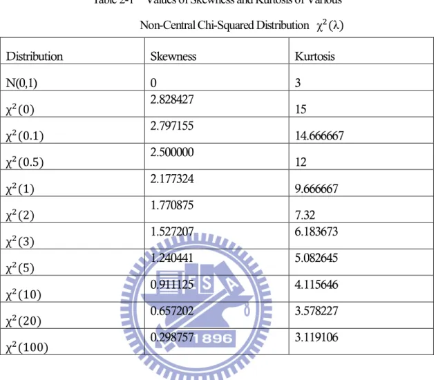
Denote the family of non-central chi-squared distributions with mean (1 + λ) and degree of freedom 1 by χ (λ). The non-central chi-squared distributions are skewed. To see how this distribution is different from the standard normal distribution in terms of skewness and kurtosis, Table 2-1 presents the values of skewness and kurtosis (which are defined as the third and fourth moments of the standardized distribution, respectively) of the non-central chi-squared distributions under study. The skewness and kurtosis of χ (λ) are √8(1 + 3λ) (1 + 2λ) / _and

3+12(1 + 4λ) (1 + 2λ)⁄ respectively. We can find in Table 2-1 when the λ decreases, the corresponding values of skewness and kurtosis will become large and far away from the values of the standard normal distribution. The result through these distributions, we can get some insights of the effects of non-normality in terms of skewness and kurtosis. Fig. 2-1 presents several non-central chi-squared distributions along with a normal distribution for the same mean and variance. In this study, we let λ= 0.1, 0.5, 1, 2, 3, 5, 10, 20 and 100, when ν=1. As can be seen from Fig. 2-1 a–f, as λ increases, the non-central chi-squared distribution appears more nearly normal distribution. In fact, we demonstrate this convergence property in Table 2-1, by calculating the skewness and kurtosis. It can be seen that as λ increases, the skewness and kurtosis of non-central chi-squared distribution are very close to those of normal distribution. Through these distributions, we wish to get some insights of the effects of non-normality on the detection power in terms of skewness and kurtosis in Section 2.

(14)

6

Table 2-1 Values of Skewness and Kurtosis of Various Non-Central Chi-Squared Distribution χ (λ)

Distribution Skewness Kurtosis

N(0,1) 0 3 χ (0) 2.828427 15 χ (0.1) 2.797155 14.666667 χ (0.5) 2.500000 12 χ (1) 2.177324 9.666667 χ (2) 1.770875 7.32 χ (3) 1.527207 6.183673 χ (5) 1.240441 5.082645 χ (10) 0.911125 4.115646 χ (20) 0.657202 3.578227 χ (100) 0.298757 3.119106

(15)

7

Fig. 2-1 (a) Probability density functions for χ (0.1) and N(1.1, 2.4). (b) Probability density functions for χ (1) and N(2, 6). (c) Probability density functions for χ (5) and N(6, 22). (d) Probability density functions for χ (10) and N (11, 42). (e) Probability density functions for χ (100) and N(102, 402). (f) Probability density functions for χ (1000) and N(1001, 4002).

(16)

8

2.2 Statistical Properties of Non-Central Squared Distribution

The non-central chi-squared distribution has a reproductive property: If X1 and X2 are

independent random variables and each has a non-central chi-squared distribution with possible different values of ν1, ν2 of ν, and λ1, λ2 of λ, then X1+X2 also has a non-central chi-squared

distribution, with ν=ν1+ν2, and with λ=λ1+λ2. Applying this property, let X1, X2, …, Xn be a

sequence of independent distribution of χ (λ)_{and then the distribution of X}1+X2+…+Xn is

χ (nλ) . Using simply statistical technique, we can conclude that Xn~χ (nλ) n⁄ .

The standard deviation of the Xn distribution, σ ，is calculated from its relationship to the

distribution parameters and the subgroup size n as follows:

1

(1 2 )

X _n



 



Let X1, X2, …, Xn be a sequence of independent distribution of χ (3) and we plot the probability

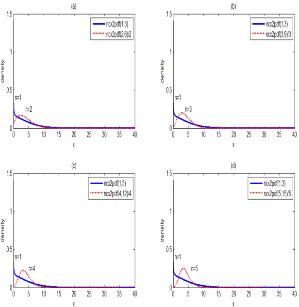
density function of the average Xn for subgroup size n=2(1)5 in Fig. 2-2 a–d. We can find that the variance of average Xn will get smaller as subgroup size n increases. This situation means that the distribution of Xn is more centralized when n>1. Also, Fig. 2-3 a-d presents several non-central chi-squared distributions of the average Xn for subgroup size n=2(1)5 along with a normal distribution for the same mean and variance. As can be seen from Fig. 2-3 a–d as n increases, the non-central chi-squared distribution of the average Xn appears more nearly normal distribution.

(17)

9

Fig. 2-2 (a) Probability density functions for χ (3) and Xn_{for n =2. (b) Probability density}

functions for χ (3) and Xn_{for n =3. (c) Probability density functions for χ (3) and}

(18)

10

Fig. 2-3 (a) Probability density functions of Xn_{for n =2, χ (2,6)/2, and N(4,7). (b) Probability}

density functions of Xn_{for n =3, χ (3,9)/3, and N(4,14/3). (c) Probability density}

functions of Xn_{for n =4, χ (4,14)/4, and N(4,4).(d) Probability density functions of}

(19)

11

3 Process Mean Shift Investigation for Non-Central

Chi-Squared Process

3.1 The Detection Power of Non-Central Chi-Squared Process

Under Bothe’s Adjustment

The major purpose of individuals control chart is assisting on identifying shifts and drifts in processes and it is easily to be implemented. But, some assumptions should be satisfied before control charts are used. The assumptions include that the process characteristics must follow normal distributions. Actually, non-normal processes occur frequently in practice. Due to above-mentioned statements, we replace the traditional, μ ± 3σ, to be the upper or lower control limits by the quantile of cumulative distribution function for different parameters of χ_υ(λ) ( F _. _{, ,} and F . , , ) and detect the power of non-central chi-squared process under Bothe’s capability

adjustments.

Let X1, X2, …, Xn be a sequence observations of independent and identically distributed

in χ (λ). Using the reproductive property of non-central chi-squared distribution, the mean of the observations is Xn which is distributed in χ (nλ) n⁄ . Also, we can obtain that μ = μ =1+λ, σ = 2(1 + 2λ) and σ = 2(1 + 2λ) n⁄ . Consequently, we derived the power of non-central chi-squared process as follows. Since the type II error β is

1 0 0.00135, , 0.99865, , ( , ) 0.99865, , ( , ) 0.00135, , ( | ) ( ) = ( ) ( ) , i i i i i i n _X n n n X X n n X n n n X n n n X P LCL X UCL k P F k X k F k F k F k                               

(20)

12

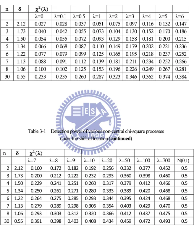
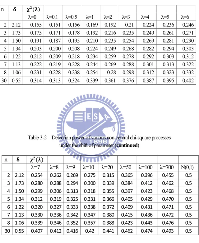
where 1-β is the detection power of the process, Φ_{( ,λ)}(∙) is the cumulative distribution function of χ (nλ)/n.The control limits LCL and UCL are calculated as _. _{, ,} and _. _{, ,} , respectively. Table 3-1presents the detection power under the alternative hypothesis test, the mean shift caused by the shift of location δ, when data comes from non-central chi-squared distribution with λ=0, 0.1, 0.5, 1(1)10, 20, 50, 100, and 700. Table 3-2 presents the detection power under the alternative hypothesis test, the mean shift caused by the shift of the parameter λ, when data comes from non-central chi-squared distribution with λ=0, 0.1, 0.5, 1(1)10, 20, 50, 100, and 700. The magnitude of shift in the second row on the left is Bothe’s capability adjustments determined when data comes from normal distribution and the detection power is 0.5. From Table 3-1, we can find that the detection power is less than 0.5 when data comes from non-central chi-squared distribution under Bothe’s capability adjustments. Our study shows that the detection power gets closer to 0.5 as λ increases, which is reasonable since the corresponding distributions get closer to the standard normal distribution. This is due to Bothe’s (2002) approach is based on the normality assumption of the data and the detection power is 0.5. The skewness of χ (λ) is √8(1 + 3λ) (1 + 2λ) / _.

Therefore, as λ decreases the non-central chi-squared distribution is more skewed and the detection power is poorer. For example, when λ= 0.5 and the subgroup size n=2, the detection power is 0.037. It implies Bothe’s adjustments are inadequate when we have skewed processes. Consequently, in our study, we determined the capability adjustment and calculation when process data comes from non-central chi-squared distribution.

(21)

13

Table 3-1 Detection power of various non-central chi-square processes under the shift of location

n ( ) λ=0 λ=0.1 λ=0.5 λ=1 λ=2 λ=3 λ=4 λ=5 λ=6 2 2.12 0.027 0.028 0.037 0.051 0.075 0.097 0.116 0.132 0.147 3 1.73 0.040 0.042 0.055 0.073 0.104 0.130 0.152 0.170 0.186 4 1.50 0.054 0.055 0.072 0.093 0.129 0.158 0.181 0.200 0.215 5 1.34 0.066 0.068 0.087 0.110 0.149 0.179 0.202 0.221 0.236 6 1.22 0.077 0.079 0.099 0.125 0.165 0.195 0.218 0.237 0.252 7 1.13 0.088 0.091 0.112 0.139 0.181 0.211 0.234 0.252 0.266 8 1.06 0.100 0.102 0.125 0.153 0.196 0.226 0.249 0.267 0.281 30 0.55 0.233 0.235 0.260 0.287 0.323 0.346 0.362 0.374 0.384

Table 3-1 Detection power of various non-central chi-square processes under the shift of location (continued)

n ( ) λ=7 λ=8 λ=9 λ=10 λ=20 λ=50 λ=100 λ=700 N(0,1) 2 2.12 0.160 0.172 0.182 0.192 0.256 0.332 0.377 0.452 0.5 3 1.73 0.200 0.212 0.222 0.232 0.293 0.360 0.398 0.460 0.5 4 1.50 0.229 0.241 0.251 0.260 0.317 0.379 0.412 0.466 0.5 5 1.34 0.250 0.261 0.271 0.280 0.333 0.389 0.420 0.468 0.5 6 1.22 0.264 0.275 0.285 0.293 0.344 0.395 0.424 0.468 0.5 7 1.13 0.279 0.289 0.298 0.306 0.354 0.403 0.429 0.470 0.5 8 1.06 0.293 0.303 0.312 0.320 0.366 0.412 0.437 0.475 0.5 30 0.55 0.391 0.398 0.403 0.408 0.434 0.459 0.472 0.493 0.5

(22)

14

Table 3-2 Detection power of various non-central chi-square processes under the shift of parameter

n ( ) λ=0 λ=0.1 λ=0.5 λ=1 λ=2 λ=3 λ=4 λ=5 λ=6 2 2.12 0.155 0.151 0.156 0.169 0.192 0.21 0.224 0.236 0.246 3 1.73 0.175 0.171 0.178 0.192 0.216 0.235 0.249 0.261 0.271 4 1.50 0.191 0.187 0.195 0.210 0.235 0.254 0.269 0.281 0.290 5 1.34 0.203 0.200 0.208 0.224 0.249 0.268 0.282 0.294 0.303 6 1.22 0.212 0.209 0.218 0.234 0.259 0.278 0.292 0.303 0.312 7 1.13 0.222 0.219 0.228 0.244 0.269 0.288 0.301 0.313 0.322 8 1.06 0.231 0.228 0.238 0.254 0.28 0.298 0.312 0.323 0.332 30 0.55 0.314 0.313 0.324 0.339 0.361 0.376 0.387 0.395 0.402

Table 3-2 Detection power of various non-central chi-square processes under the shift of parameter (continued)

n ( ) λ=7 λ=8 λ=9 λ=10 λ=20 λ=50 λ=100 λ=700 N(0,1) 2 2.12 0.254 0.262 0.269 0.275 0.315 0.365 0.396 0.455 0.5 3 1.73 0.280 0.288 0.294 0.300 0.339 0.384 0.412 0.462 0.5 4 1.50 0.299 0.306 0.313 0.318 0.355 0.397 0.423 0.468 0.5 5 1.34 0.312 0.319 0.325 0.331 0.366 0.405 0.429 0.470 0.5 6 1.22 0.320 0.327 0.333 0.338 0.372 0.409 0.431 0.471 0.5 7 1.13 0.330 0.336 0.342 0.347 0.380 0.415 0.436 0.472 0.5 8 1.06 0.339 0.346 0.352 0.357 0.388 0.423 0.443 0.476 0.5 30 0.55 0.407 0.412 0.416 0.42 0.441 0.462 0.474 0.493 0.5

(23)

15

3.2 The Modified Mean Adjustments for Non-Central

Chi-Squared Process

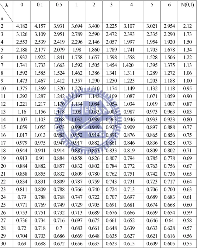
The undetected mean shift adjustment cause by the shift of location δ in Table 3-3 is called AS50

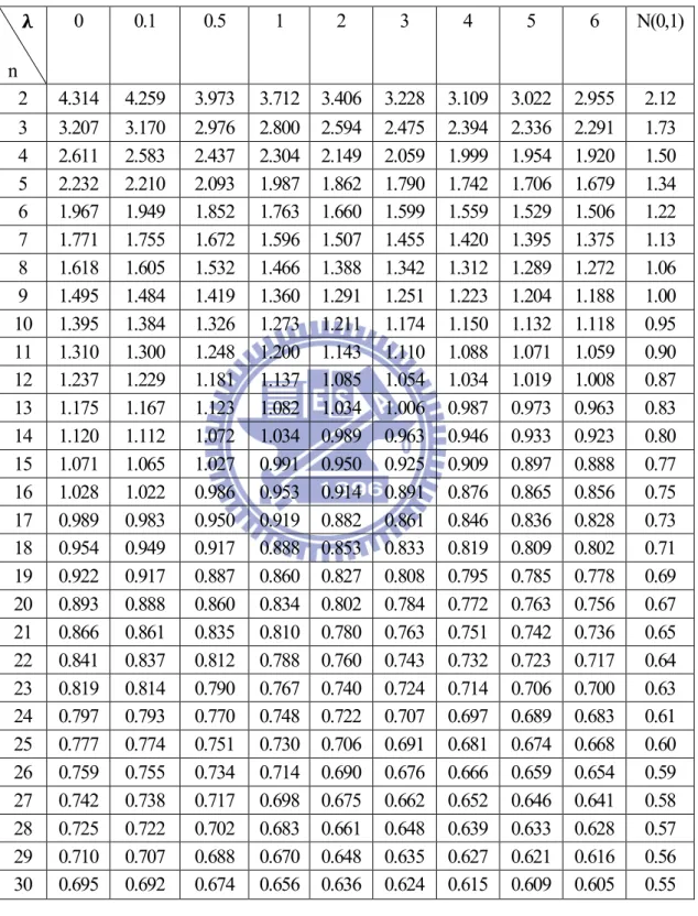
which is the magnitude of shift we need to adjust based on designated detection power is 0.5 and process data comes from non-central chi-squared distribution. The undetected mean shift adjustment causeby the shift of parameter λ in Table 3-4 is called AS50 which is the magnitude of

shift we need to adjust based on designated detection power is 0.5 and process data comes from non-central chi-squared distribution. Table 3-3 and Table 3-4 display the magnitude of adjustments AS50 based on the detection power is 0.5 and data comes from χ (λ) with various values of

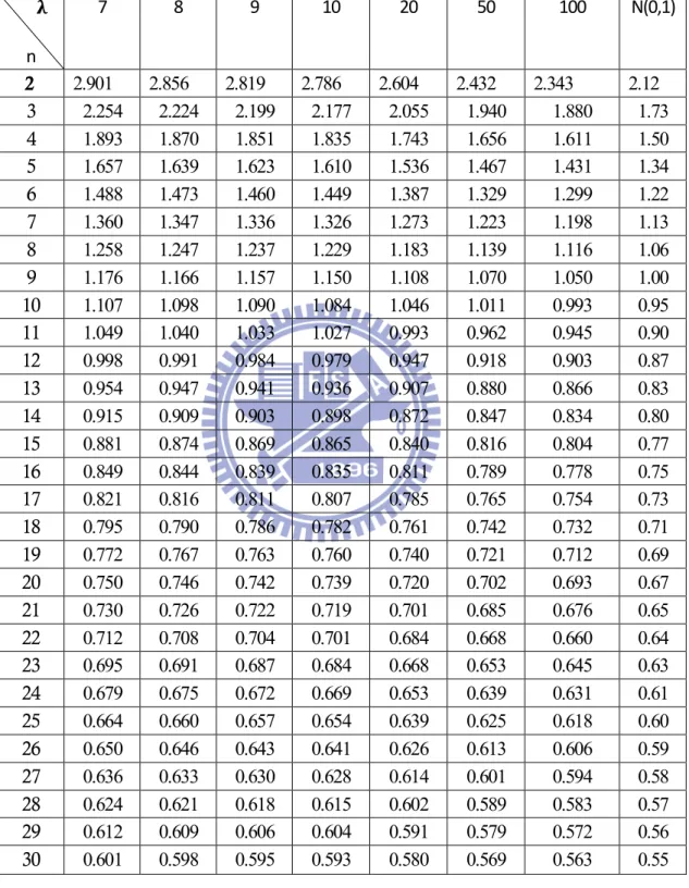
λ(=0.1, 0.5, 1(1)10, 20, 50, and 100 ) and n=2(1)30. For example, if we set λ=3 and n=5, then the adjustment from Table 3-3 is AS50=1.79. We conclude that the adjustment AS50σ (=1.79σ) is

required based on the detection power is 0.5 and data comes from χ (λ). It also shows from Table 3-3 that the adjustments AS50 get closer to Bothe’s adjustments as λ increases (when n=2(1)10),

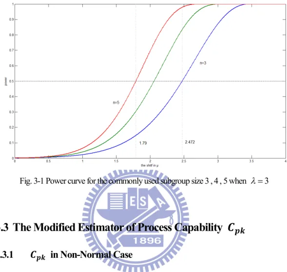
which is reasonable since the corresponding distributions get closer to the standard normal distribution. However, we should notice that when λ is small (distribution is strongly skewed), the required adjustment in the capability index formula is much greater than those for normal processes. Using the adjusted process capability formula, the engineers can determine the actual process capability more accurately. Fig. 3-1 presents the power curves, these lines on the graph depict the probabilities of detecting a shift in μ for the commonly used subgroup size n=3, 4, 5 (expressed in σ units on the horizontal axis) when λ=3. All these lines are close to zero for small shifts in μ. It can be found that the power of the chart with all three curves eventually leveling off close to 100% as the size of the shifts in excess of 3.5σ. The dashed horizontal line drawn in Fig. 3-1 shows that there is a 50% probability of missing a 1.79σ shift in μ when n is 5, while μ must move by 2.472σ to have this same probability when n is only 3. The shift sizes that have a 50% probability

(24)

16

of remaining undetected, called AS50 values are listed in Table 3-3 for subgroup sizes n=2(1)30.

Momentary movements in μ smaller than AS50σ are more than likely to be missed by a control

chart. Therefore our adjustment AS50 takes into account those shifts that are not detected by the

(25)

17

Table 3-3 AS50 values for several subgroup size n and various λ values

under the shift of location n 0 0.1 0.5 1 2 3 4 5 6 N(0,1) 2 4.182 4.157 3.931 3.694 3.400 3.225 3.107 3.021 2.954 2.12 3 3.126 3.109 2.951 2.789 2.590 2.472 2.393 2.335 2.290 1.73 4 2.553 2.539 2.419 2.296 2.146 2.057 1.997 1.954 1.920 1.50 5 2.188 2.177 2.079 1.98 1.860 1.789 1.741 1.705 1.678 1.34 6 1.932 1.922 1.841 1.758 1.657 1.598 1.558 1.528 1.506 1.22 7 1.741 1.733 1.663 1.592 1.505 1.454 1.420 1.395 1.375 1.13 8 1.592 1.585 1.524 1.462 1.386 1.341 1.311 1.289 1.272 1.06 9 1.473 1.467 1.412 1.357 1.290 1.250 1.223 1.203 1.188 1.00 10 1.375 1.369 1.320 1.270 1.210 1.174 1.149 1.132 1.118 0.95 11 1.292 1.287 1.242 1.197 1.142 1.109 1.087 1.071 1.059 0.90 12 1.221 1.217 1.176 1.134 1.084 1.054 1.034 1.019 1.007 0.87 13 1.16 1.156 1.118 1.08 1.033 1.005 0.987 0.973 0.963 0.83 14 1.107 1.103 1.068 1.032 0.989 0.963 0.946 0.933 0.923 0.80 15 1.059 1.055 1.023 0.990 0.949 0.925 0.909 0.897 0.888 0.77 16 1.017 1.013 0.983 0.952 0.914 0.891 0.876 0.865 0.856 0.75 17 0.979 0.975 0.947 0.917 0.882 0.861 0.846 0.836 0.828 0.73 18 0.944 0.941 0.914 0.887 0.853 0.833 0.819 0.809 0.802 0.71 19 0.913 0.91 0.884 0.858 0.826 0.807 0.794 0.785 0.778 0.69 20 0.884 0.882 0.857 0.832 0.802 0.784 0.772 0.763 0.756 0.67 21 0.858 0.855 0.832 0.809 0.780 0.762 0.751 0.742 0.736 0.65 22 0.834 0.831 0.809 0.787 0.759 0.743 0.731 0.723 0.717 0.64 23 0.811 0.809 0.788 0.766 0.740 0.724 0.713 0.706 0.700 0.63 24 0.79 0.788 0.768 0.747 0.722 0.707 0.697 0.689 0.683 0.61 25 0.771 0.769 0.749 0.729 0.705 0.691 0.681 0.674 0.668 0.60 26 0.753 0.751 0.732 0.713 0.689 0.676 0.666 0.659 0.654 0.59 27 0.736 0.734 0.716 0.697 0.675 0.661 0.652 0.646 0.64 0.58 28 0.72 0.718 0.7 0.683 0.661 0.648 0.639 0.633 0.628 0.57 29 0.704 0.703 0.686 0.669 0.648 0.635 0.627 0.621 0.616 0.56 30 0.69 0.688 0.672 0.656 0.635 0.623 0.615 0.609 0.605 0.55

(26)

18

under the shift of location (continued) n 7 8 9 10 20 50 100 N(0,1) 2 2.900 2.856 2.818 2.786 2.604 2.432 2.343 2.12 3 2.254 2.224 2.199 2.177 2.055 1.940 1.880 1.73 4 1.893 1.870 1.851 1.835 1.743 1.656 1.611 1.50 5 1.656 1.638 1.623 1.610 1.536 1.467 1.431 1.34 6 1.487 1.472 1.460 1.449 1.387 1.329 1.299 1.22 7 1.359 1.346 1.336 1.326 1.273 1.223 1.198 1.13 8 1.258 1.247 1.237 1.229 1.183 1.139 1.116 1.06 9 1.176 1.166 1.157 1.150 1.108 1.070 1.050 1.00 10 1.107 1.098 1.090 1.084 1.046 1.011 0.993 0.95 11 1.049 1.040 1.033 1.027 0.993 0.962 0.945 0.90 12 0.998 0.991 0.984 0.979 0.947 0.918 0.903 0.87 13 0.954 0.947 0.941 0.936 0.907 0.880 0.866 0.83 14 0.915 0.909 0.903 0.898 0.872 0.847 0.834 0.80 15 0.880 0.874 0.869 0.865 0.840 0.816 0.804 0.77 16 0.849 0.844 0.839 0.835 0.811 0.789 0.778 0.75 17 0.821 0.816 0.811 0.807 0.785 0.765 0.754 0.73 18 0.795 0.790 0.786 0.782 0.761 0.742 0.732 0.71 19 0.772 0.767 0.763 0.759 0.740 0.721 0.712 0.69 20 0.750 0.746 0.742 0.739 0.720 0.702 0.693 0.67 21 0.730 0.726 0.722 0.719 0.701 0.685 0.676 0.65 22 0.712 0.708 0.704 0.701 0.684 0.668 0.660 0.64 23 0.695 0.691 0.687 0.684 0.668 0.653 0.645 0.63 24 0.679 0.675 0.672 0.669 0.653 0.639 0.631 0.61 25 0.664 0.660 0.657 0.654 0.639 0.625 0.618 0.60 26 0.650 0.646 0.643 0.640 0.626 0.613 0.606 0.59 27 0.636 0.633 0.630 0.628 0.614 0.601 0.594 0.58 28 0.624 0.621 0.618 0.615 0.602 0.589 0.583 0.57 29 0.612 0.609 0.606 0.604 0.591 0.579 0.572 0.56 30 0.601 0.598 0.595 0.593 0.580 0.569 0.563 0.55

(27)

19

under the shift of parameter n 0 0.1 0.5 1 2 3 4 5 6 N(0,1) 2 4.314 4.259 3.973 3.712 3.406 3.228 3.109 3.022 2.955 2.12 3 3.207 3.170 2.976 2.800 2.594 2.475 2.394 2.336 2.291 1.73 4 2.611 2.583 2.437 2.304 2.149 2.059 1.999 1.954 1.920 1.50 5 2.232 2.210 2.093 1.987 1.862 1.790 1.742 1.706 1.679 1.34 6 1.967 1.949 1.852 1.763 1.660 1.599 1.559 1.529 1.506 1.22 7 1.771 1.755 1.672 1.596 1.507 1.455 1.420 1.395 1.375 1.13 8 1.618 1.605 1.532 1.466 1.388 1.342 1.312 1.289 1.272 1.06 9 1.495 1.484 1.419 1.360 1.291 1.251 1.223 1.204 1.188 1.00 10 1.395 1.384 1.326 1.273 1.211 1.174 1.150 1.132 1.118 0.95 11 1.310 1.300 1.248 1.200 1.143 1.110 1.088 1.071 1.059 0.90 12 1.237 1.229 1.181 1.137 1.085 1.054 1.034 1.019 1.008 0.87 13 1.175 1.167 1.123 1.082 1.034 1.006 0.987 0.973 0.963 0.83 14 1.120 1.112 1.072 1.034 0.989 0.963 0.946 0.933 0.923 0.80 15 1.071 1.065 1.027 0.991 0.950 0.925 0.909 0.897 0.888 0.77 16 1.028 1.022 0.986 0.953 0.914 0.891 0.876 0.865 0.856 0.75 17 0.989 0.983 0.950 0.919 0.882 0.861 0.846 0.836 0.828 0.73 18 0.954 0.949 0.917 0.888 0.853 0.833 0.819 0.809 0.802 0.71 19 0.922 0.917 0.887 0.860 0.827 0.808 0.795 0.785 0.778 0.69 20 0.893 0.888 0.860 0.834 0.802 0.784 0.772 0.763 0.756 0.67 21 0.866 0.861 0.835 0.810 0.780 0.763 0.751 0.742 0.736 0.65 22 0.841 0.837 0.812 0.788 0.760 0.743 0.732 0.723 0.717 0.64 23 0.819 0.814 0.790 0.767 0.740 0.724 0.714 0.706 0.700 0.63 24 0.797 0.793 0.770 0.748 0.722 0.707 0.697 0.689 0.683 0.61 25 0.777 0.774 0.751 0.730 0.706 0.691 0.681 0.674 0.668 0.60 26 0.759 0.755 0.734 0.714 0.690 0.676 0.666 0.659 0.654 0.59 27 0.742 0.738 0.717 0.698 0.675 0.662 0.652 0.646 0.641 0.58 28 0.725 0.722 0.702 0.683 0.661 0.648 0.639 0.633 0.628 0.57 29 0.710 0.707 0.688 0.670 0.648 0.635 0.627 0.621 0.616 0.56 30 0.695 0.692 0.674 0.656 0.636 0.624 0.615 0.609 0.605 0.55

(28)

20

under the shift of parameter (continued) n 7 8 9 10 20 50 100 N(0,1) 2 2.901 2.856 2.819 2.786 2.604 2.432 2.343 2.12 3 2.254 2.224 2.199 2.177 2.055 1.940 1.880 1.73 4 1.893 1.870 1.851 1.835 1.743 1.656 1.611 1.50 5 1.657 1.639 1.623 1.610 1.536 1.467 1.431 1.34 6 1.488 1.473 1.460 1.449 1.387 1.329 1.299 1.22 7 1.360 1.347 1.336 1.326 1.273 1.223 1.198 1.13 8 1.258 1.247 1.237 1.229 1.183 1.139 1.116 1.06 9 1.176 1.166 1.157 1.150 1.108 1.070 1.050 1.00 10 1.107 1.098 1.090 1.084 1.046 1.011 0.993 0.95 11 1.049 1.040 1.033 1.027 0.993 0.962 0.945 0.90 12 0.998 0.991 0.984 0.979 0.947 0.918 0.903 0.87 13 0.954 0.947 0.941 0.936 0.907 0.880 0.866 0.83 14 0.915 0.909 0.903 0.898 0.872 0.847 0.834 0.80 15 0.881 0.874 0.869 0.865 0.840 0.816 0.804 0.77 16 0.849 0.844 0.839 0.835 0.811 0.789 0.778 0.75 17 0.821 0.816 0.811 0.807 0.785 0.765 0.754 0.73 18 0.795 0.790 0.786 0.782 0.761 0.742 0.732 0.71 19 0.772 0.767 0.763 0.760 0.740 0.721 0.712 0.69 20 0.750 0.746 0.742 0.739 0.720 0.702 0.693 0.67 21 0.730 0.726 0.722 0.719 0.701 0.685 0.676 0.65 22 0.712 0.708 0.704 0.701 0.684 0.668 0.660 0.64 23 0.695 0.691 0.687 0.684 0.668 0.653 0.645 0.63 24 0.679 0.675 0.672 0.669 0.653 0.639 0.631 0.61 25 0.664 0.660 0.657 0.654 0.639 0.625 0.618 0.60 26 0.650 0.646 0.643 0.641 0.626 0.613 0.606 0.59 27 0.636 0.633 0.630 0.628 0.614 0.601 0.594 0.58 28 0.624 0.621 0.618 0.615 0.602 0.589 0.583 0.57 29 0.612 0.609 0.606 0.604 0.591 0.579 0.572 0.56 30 0.601 0.598 0.595 0.593 0.580 0.569 0.563 0.55

(29)

21

Fig. 3-1 Power curve for the commonly used subgroup size 3 , 4 , 5 when  3

3.3 The Modified Estimator of Process Capability

3.3.1 in Non-Normal Case

The index Cpk has been viewed as a yield-based index since it provides bounds on the process

yield for a normally distributed process with a fixed value of Cpk. This index Cpk is defined as:

C

min{

,

} ,

3

pk

USL

 

LSL







where as above USL is the upper specification limit, LSL is the lower specification limit, μ is the process mean and σ is the process standard deviation. The proper use of process capability indices, which are statistical measures of process capability, is based on several assumptions. One of the most essential is that the process monitored is supposed to be stable and the output is approximately

(30)

22

normally distributed. When the distribution of a process characteristic is non-normal, PCIs calculated using conventional methods could often lead to erroneous and misleading interpretation of the process’s capability.

In the recent years, several approaches to problems of PCIs for the non-normal populations have been suggested. A widely accepted approach for PCI computation is to use the popular normal plot so that the normality assumption can be verified simultaneously. Analogous to the normal probability plot, where the “nature” process width is between the 0.135 percentile and 99.865 percentile, surrogate PCI values may be obtained via appropriately selected probability plots. Since the median is usually the preferable central value for a skewed distribution, the corresponding Cpu

and Cpl are defined as:

0.5 0.99865 0.5

(

0.135% point)

pu

USL

F

USL

median

C

upper

median

F







0.5 0.5 0.00135

(

0.135% point)

pl

F

LSL

median

LSL

C

median

lower

F







Then the index Cpk would be calculated as the minimum of Cpu and Cpl, namely:

0.5 0.5 0.99865 0.5 0.5 0.00135 min{ , } min{ , } pk pu pl USL F F LSL C C C F F F F      

so that the normality assumption can be verified simultaneously

.

We can obtain more accurate measures of these percentile points (F0.00135, F0.5 and F0.99865)

under consideration in the non-normal case, if we are able to find a better distributional form for the data, which provides a very satisfactory fit. This involves modeling the process data with alternative probability plot models, such as the Weibull or gamma ones (see e.g. Dudewicz and Mishra, 1998;

(31)

23

Kotz and Lovelace, 1998). Nevertheless, an obvious disadvantage of probability plotting is that it is not a truly objective procedure. It is quite possible for two analysts to arrive at different conclusions using the same data. Accordingly, it is often desirable to supplement probability plots with goodness-of-fit tests, which possess more formal statistical foundations (see, e.g., Shapiro, 1995). Choosing proper distribution to fit the data is an important step in probability plotting. Sometimes one can use the available knowledge of the physical phenomenon or the past experience to suggest a choice of the distribution.

3.3.2 Adjustment of

Acknowledging that a process will experience shift in F0.5 of various magnitudes and knowing

that not all of these will be discovered, some allowance for them must be made when estimating outgoing quality so customers are not disappointed. Because shifts ranging in size from 0 to AS50σ

are the ones likely to remain undetected (large moves should be caught by the chart), a conservative approach is to assume that every missed shift is as large as AS50.

Considering the undetected process mean shift as large as AS50σ, we use F0.5 minus AS50σ to

evaluate how well the process output meets the LSL and F0.5 plus AS50σ for determining

conformance to the USL when estimating the index Cpk . Incorporating both of these adjustments

into the basic Cpk formula we obtained the ‘‘dynamic’’ Cpk index by making the following

modifications: 0.5 50 0.5 50 0.99865 0.5 0.5 0.00135 0.5 50 0.5 50 0.99865 0.5 0.99865 0.5 0.5 0.00135 0.5 0.00135

(

) (

)

min{

,

}

(

= min{

,

}

pk

USL

F

AS

F

AS

LSL

C

F

USL

F

AS

F

LSL

AS

F













(32)

24

By considering an adjustment AS50σ in this assessment for undetected shifts in process median, the

estimate of dynamic index Cpk will decrease and the expected total number of nonconforming parts

will increase. It must be noticed that this nonconforming level assumes that undetected shifts are happening almost constantly and that everyone is equal to AS50σ. From Table 3-3, the practitioners

can find the AS50 to calculate the dynamic index Cpk for determining whether their process meets

(33)

25

4 Application

Recently, due to the excellent current driving capability and microwave performances, heterojunction bipolar transistors (HBTs) have extensively employed on digital and analogy applications and are recognized as promising electronic devices for high frequency and high performance circuit applications, such as monolithic microwave integrated circuit and optoelectronic integrated circuit. For successful process control, process optimization, circuit design, and compact transistor modeling, there are several problems that must be overcome to realize practical high speed ICs. One of the problems is a current gain reduction associated with the scaling down of transistor size. Since the emitter dimension must be minimized for higher switching speed operation, elimination of the current gain reduction is very important for HBT designs. Also, Cutoff frequency and maximum oscillation frequency were changed with emitter dimension, and this was attributed to the variation of resistances and junction capacitances with emitter structure.

Therefore, we should address on one of the characteristics of HBTs, the emitter area. The upper and lower manufacturing specific limits are set to USL=45 um2 and LSL=5 um2, respectively. If the characteristic data does not fall within the tolerance (LSL, USL) , the component of the emitter area is consider to nonconforming/defective, and will not be used to make the emitter area of that particular model.

As shown in Table 4-1, a part of historical data is collected. Fig. 4-2displays the histogram, and Fig. 4-1 displays the normal probability plot of these historical data. From the Fig. 4-1 and Fig. 4-2 , it is evident to conclude the data collected from the factory are not normal distributed. The data analysis results justify that the process is significantly away from the normal distribution. By the goodness-of-fit tests, the historical data indicates that the process pretty approximates to be distributed as non-central chi-squared. The parameter ν and λ of non-central chi-squared

(34)

26

distribution could be calculated from historical data giving ν=1 and λ=20. Therefore, it is approximate to use this approach and we can obtain more accurate measures of the three quantile:

F0.00135 , F0.5 (median) , and F0.99865 for

1 1

(1 2 ) (1 2 20) 4.1 2.025 10

n



 



    

under consideration. Then “dynamic” Cpk index can be calculated as follows:

0.5 50 0.5 50 0.99865 0.5 0.5 0.00135

)

min{

,

}

45 20 1.046 2.025 20 1.046 2.025 5

=min{

,

}

55.832 20

20 2.167

min{0.64, 0.72}

pk

USL F

AS

F

AS

LSL

dynamic C

F



















=0.64

with AS50=1.046 for n=10 from Table 3-3. Compared it to the value of the following conventional

index: 0.5 0.5 0.99865 0.5 0.5 0.00135

min{

,

}

min{

,

}

45 20

20-5

=min{

,

}

55.832-20 20-2.167

min{ 0.70,0.84}=0.70

pk pu pl

USL

F

LSL

C

F









calculated by a traditional capability study (the shift of process mean is not considered), we can find that the value of the modified Cpk is much smaller. This result indicates if the process mean shifts

that are not detected then unadjusted Cpk would overestimate the actual process yield which is not

derisible. Our adjustment takes into account those shifts that are not detected so that the practitioner would be able to keep its quality promise for this process. As the adjusted process capability drops below the desired quality level, the practitioner should stop the process because the process does not

(35)

27

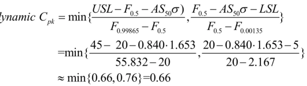
meet his preset capability requirement. As the subgroup size n increases, the shift in process mean have a higher probability of detection. For example, if n=15, the AS50 would be 0.840 for χ (20)

from Table 3-3, and then the ‘‘dynamic’’ Cpk index is

0.5 50 0.5 50 0.99865 0.5 0.5 0.00135

)

min{

,

}

45 20 0.840 1.653 20 0.840 1.653 5

=min{

,

}

55.832 20

20 2.167

min{0.66, 0.76}=0.66

pk

USL F

AS

F

AS

LSL

dynamic C

F



















Changing n from 10 to 15 increases the dynamic Cpk index from 0.64 to 0.66, and the total number

of nonconforming parts would be reduced.

Table 4-1 The 100 observations are collected from the historical data

32.955 15.736 25.510 18.311 6.255 19.248 16.3 32.922 17.451 11.374 9.858 18.385 14.725 37.943 27.512 20.158 23.992 24.408 19.497 20.954 28.506 16.812 31.125 34.926 21.003 8.116 19.456 18.011 16.695 23.67 18.49 9.844 11.532 25.789 22.311 19.973 17.759 24.597 15.493 16.397 17.771 24.566 24.018 6.658 14.296 20.389 29.304 10.274 13.462 17.752 33.647 23.895 20.944 30.906 10.373 26.093 21.52 20.644 29.198 24.368 31.458 13.159 23.962 27.004 24.527 23.57 15.256 20.438 24.599 9.911 12.983 8.23 26.109 22.977 10.126 41.423 8.854 16.815 17.774 13.339 11.316 18.924 5.114 33.823 22.43 20.686 31.242 11.123 9.868 37.314 14.859 43.001 17.45 35.999 17.945 16.318 12.035 11.187 19.182 19.607

(36)

28 -2 -1 0 1 2 1 0 2 0 3 0 4 0

Quantiles of Standard Norm

H is to ri c a l d a ta Historical data 10 20 30 40 0 5 1 0 1 5 2 0 2 5

Fig. 4-1 Normal probability plot of the historical data

(37)

29

5 Conclusions

In this paper, we considered the problem of how to determine the adjustments for process capability with mean shift when data follows the non-central chi-squared distribution. We first examined Bothe’s approach and found the detection power is less than 0.5 when data comes from the non-central chi-squared distribution, showing that Bothe’s adjustments are inadequate when we have non-central chi-squared processes. For non-central chi-squared processes, we calculated the adjustments for various sample sizes (n) and non-central chi-square parameter (ν, λ) with detection power fixed to 0.5. For small value of λ (distribution is strongly skewed), the required adjustment in the capability index formula is much greater than those for normal processes. Using the adjusted process capability formula, the engineers can determine the actual process capability more accurately. Tables are also provided for engineers/practitioners to use in their in-plant applications. A real-world semi-conductor production plant is investigated and presented to illustrate the applicability of the proposed approach.

(38)

30

Reference

[1] Bender, A. (1975). Statistical tolerancing as it relates to quality control and the designer.

Automotive Division Newsletter of ASQC.

[2] Bothe, D.R. (2002). Statistical reason for the 1.5σ shift. Quality Engineering , 14 (3), 479–487.

[3] Chan, L.K., Cheng, S.W., Spiring, F. A. (1988). A new measure of process capability Cpm.

Journal of Quality Technology 20 (3), 162–175.

[4] Choi, K.C., Nam, K.H., Park, D.H., (1996). Estimation of capability index based on bootstrap method. Microelectronics Reliability 36 (9), 1141–1153.

[5] Clements, J.A. (1989). Process capability calculations for non-normal distributions. Quality Progress, 95–100.

[6] Ding, J. (2004). A method of estimating the process capability index from the first four moments of non-normal data. Quality and Reliability Engineering International 20, 787–805. [7] Dudewicz, E.J., Mishra, S.N. (1998). Modern Mathematical Statistics. John Wiley, New York. [8] Evans, D.H. (1975). Statistical tolerancing: The state of the art, Part III: Shifts and drifts.

Journal of Quality Technology 7 (2), 72–76.

[9] Franklin, L.A., Wasserman, G.S. (1992). Bootstrap lower confidence limits for capability indices. Journal of Quality Technology 24 (4), 196–210.

[10] Gilson, J.A. (1951). New Approach to Engineering Tolerances. Machinery Publishing Co., London.

[11] Kane, V.E. (1986). Process capability indices. Journal of Quality Technology 18 (1), 41–52. [12] Kocherlakota, S., Kocherlakota, K., Kirmani, S.N.U.A. (1992). Process capability index

under non-normality. International Journal of Mathematical Statistics 1 (2), 175–210.

(39)

31

London, UK.

[14] Lucas, J.M. (1976). The design and use of cumulative sum quality control schemes. Journal

of Quality Technology 8, 1–12.

[15] Lucas, J.M., Crosier, R.B. (2000). Fast initial response for CUSUM Quality-Control schemes: Give your CUSUM a head start. Technometrics 42 (1), 102–107.

[16] Luceno, A., Puig-Pey, J. (2002). Computing the run length probability distribution of CUSUM charts. Journal of Quality Technology 34(2), 209–215.

[17] Pal, S. (2005). Evaluation of non-normal process capability indices using generalized lambda distribution. Quality Engineering 17, 77–85.

[18] Pearn, W.L., Chen, K.S. (1997). Capability indices for non-normal distributions with an application in electrolytic capacitor manufacturing. Microelectronics and Reliability 37 (12), 1853–1858.

[19] Pearn, W.L., Kotz, S., Johnson, N.L. (1992). Distributional and inferential properties of process capability indices. Journal of Quality Technology 24 (4), 216–233.

[20] Polansky, A.M. (1998). A smooth nonparametric approach to process capability. Quality

and Reliability Engineering International 14, 43–48.

[21] Pyzdek, T. (1992). Process capability analysis using personal computers. Quality

Engineering 4 (3), 419–440.

[22] Ross, S. (2005). A First Course in Probability Theory, seventh ed. Academic Press, New York.

[23] Schilling, E.G., Nelson, P.R. (1976). The effect of non-normality on the control limits of charts. Journal of Quality Technology 8, 183–188.

[24] Shapiro, S.S. (1995). Goodness-of-fit tests. In: Balakrishnan, N., Basu, A.P. (Eds.), The Exponential Distribution: Theory Methods and Applications. Gordon and Breach, Langhorne, Pennsylvania, Chapter 13.

(40)

32

[25] Shore, H. (1998). A new approach to analyzing non-normal quality data with application to process capability analysis. International Journal of Production Research 36 (7), 1917–1933.

[26] Somerville, S.E., Montgomery, D.C. (1996). Process capability indices and non-normal distributions. Quality Engineering 9 (2), 305–316.

考慮非中心卡方製程的製程平均發生偏移下之製程能力調整

國 立 交 通 大 學

統計學研究所

碩 士 論 文