數位相機彩色濾鏡陣列影像雜訊消除方法

國

立

交

通

大

學

電機學院 電機與控制學程

碩 士 論 文

數位相機彩色濾鏡陣列影像雜訊消除方法

Color Filter Array Denoising Method for Digital Cameras

研 究 生：唐學用

指導教授：林昇甫 博士

數位相機彩色濾鏡陣列影像雜訊消除方法

Color Filter Array Denoising Method for Digital Cameras

研 究 生：唐學用 Student：Hsueh-Yung Tang

指導教授：林昇甫 博士 Advisor：Dr. S. F. Lin

國 立 交 通 大 學

電機學院 電機與控制學程

碩 士 論 文

A Thesis

Submitted to College of Electrical and Computer Engineering National Chiao Tung University

in partial Fulfillment of the Requirements for the Degree of

Master of Science in

Electrical and Control Engineering January 2008

數 位 相 機 彩 色 濾 鏡 陣 列 影 像 雜 訊 消 除 方 法

學生：唐學用 指導教授

：

林昇甫 博士

國 立 交 通 大 學 電 機 學 院 電 機 與 控 制 學 程 碩 士 班

摘

要

當今時下，數位相機已幾乎完全取代傳統底片相機，舊有的底片也有

產品將之翻拍成數位照片，這個趨勢已如潮水般滾滾而來，不只是數位相

機，舉凡能數位化的產品都逃不過數位化的命運，只因數位資訊便於處理、

儲存以及傳遞。

數位相機中的影像處理是經過了很多道的程序而成，幾乎所有的程序都

會增強雜訊的作用，所以降低雜訊的影響最好的辦法就是在任何影像處理

的程序之前就先將影像來源本身具有的雜訊濾除掉，而影像雜訊濾除最困

難的就是在濾除雜訊的同時也保存了影像的輪廓和高頻訊號。本篇論文提

出了另一種消除影像雜訊的架構，由三個想法所組成，一個是在影像區塊

中將正在處理的像素歸類給某一預設圖樣，既然可被歸類給某一圖樣，就

可以對這圖樣中的元素平均以降低雜訊，另一個是獲取校正過後的相機雜

訊特性，掃瞄出其雜訊特性並以標準差來表示，以便於用來判別正在處理

的影像區塊是否可以判定為均勻影像，進而做出最強的濾除效果。最後一

個是運用肉眼視覺系統不易察覺到那些藏在多紋路、高反差區域的影像雜

訊，所以不去濾除那些不易被察覺的雜訊以保存更多的影像輪廓訊號。

Color Filter Array Denoising Method for Digital Cameras

Student：Hsueh-Yung Tang Advisors：Dr. S. F. Lin

Degree Program of Electrical and Computer Engineering

National Chiao Tung University

ABSTRACT

Nowadays, traditional film camera has almost been replaced by digital

camera in commercial market. This trend is not only on camera, but also on any

product in which the signal can be digitalized, since digital information would

be much convenience to be processed, stored, and transmitted.

Image processing in digital camera consists of many processes. Almost all

of the processes would enhance noise added in images. The best way to make

noise strength be minimized is to reduce noise in front of any image processing.

The difficulty of image denoising is always to preserve edge information, and

filters out noise in flat area simultaneously. In this paper, we have presented a

denoising method which consists of three ideas. One is to filter noisy pixel based

on nearest pattern to keep edge information, another one is to use camera noise

characteristic to judge the uniformity of current processed area and the last one

is to make use of the property of spatial masking to keep edge information again

on the highly texture area.

誌

謝

這篇論文的完成要感謝的人很多，有些是實質在論文上的指導，有些則是精神上的 體貼和關心。首先最要感謝的是幫助我很多的指導教授 林昇甫博士，感謝林教授的多 方幫助，包含論文的研究、生活處事哲理上的一切耐心教導，讓我受用無窮，有了林教 授的體諒和鼓勵，我們這些學生們才有辦法工作、家庭與學業兼顧，並完成此論文。也 深深感受到口試委員廖德誠教授、潘晴財教授、張翔教授等口試委員的用心和一絲不笱 的作論文態度，他們訂正了我許多地方，所提供的寶貴意見讓我受益良多。 感謝亞洲光學集團-世界宏景主管的體諒，同意讓我繼續進修，感謝同仁們分擔掉我 的工作量，特別感謝同仁林璟憲修改了相機的程式，讓我可以運用真實相機方便的比較 不同的濾雜訊方法。能進到數位相機這領域也要感謝前一家公司華晶科技，華晶科技提 供的舞台讓我和數位相機結下不解之緣，也感謝學長彭永薰和呂龍騰，由於他們的引進 才讓我可以進入這行。還有多位同仁彼此間多年下來建立出來的信任和情感，無形中也 成為我的精神支柱，感謝他們。 感謝我的父母、大哥、大嫂及家人們的關心和幫忙，也感謝恩師王瑞材教授多年來 一再的關心和噓寒問暖，每次接到王教授的電話都會有暖上心房的感覺。最後要感謝我 的太太，五年前她幫我偷偷買了簡章，在不知情的情況下，幫我把大部分的報考資料準 備好了，雖然一路上在工作、家庭和學業都要兼顧很辛苦，但她總會在需要時給我一整 段的時間讓我好好準備課業，才有完成學業的可能！ 要感謝的親朋好友很多，不及備載，儘致上最深的謝意，謝謝您們！

Contents

Abstract in Chinese ……….……….……….….i

Abstract in English ……….……….….….ii

Acknowledgements in Chinese ………..……..iii

Contents ……….…….…………...……….……….….………iv

List of Tables ………..……….….…….….v

List of Figures ……….……….………….vi

Chapter 1 Introduction ... 1

1.1 Motivation and Contribution ...1

1.2 Outline ...2

Chapter 2 Review of Related Works... 3

2.1 Color Filter Array ...3

2.2 Bilinear Method...5

2.3 Human Visual System ...5

2.4 Bosco-and-Mancuso Filter for Image Denoising ...6

2.5 Peak Signal to Noise Ratio ... 11

2.6 Structural Similarity ...12

Chapter 3 Proposed Image Noise Reduction System ... 13

3.1 Overview of Image Processing on Digital Camera ...13

3.2 Block Diagram of Proposed Denoising Method ...17

3.3 Algorithm of Proposed Denoising Method...18

Chapter 4 Experiments ... 24

4.1 Test Results of the Images with Additive Noise:...24

4.2 Test Results of the CFA Raw Images: ...53

Chapter 5 Conclusions ... 61

List of Tables

Table 01 Proposed SSIM and PSNR compare with other filters for the images with additive Gaussian random noise……….…………25 Table 02 Proposed SSIM and PSNR compare with other filters for the images with additive

Rayleigh random noise……….………26 Table 03 Proposed SSIM and PSNR compare with other filters for the images with additive

Gamma random noise………...…………27 Table 04 Proposed SSIM and PSNR compare with other filters for the images with additive

Exponential random noise……….………28 Table 05 Proposed SSIM and PSNR compare with other filters for the images with additive

Uniform random noise………...…………...…29 Table 06 Proposed SSIM and PSNR compare with other filters for the images with additive

Pepper-and-Salt random noise………..……30 Table 07 Test result of filtering image “4.1.08-jellybeansg” with additive σ=7.1875 and

σ=3.125 Gaussian noise………..…..41 Table 08 Use image “1.2.03-straw” as an example to explain the proposed filter has worst

SSIM on texture images under high Gamma noise condition……….….41 Table 09 Proposed SSIM and PSNR compare with other filters for the pattern images with

additive Gaussian noise……….…………47 Table 10 Proposed SSIM and PSNR compare with other filters for the pattern images with

additive Rayleigh noise……….…………48 Table 11 Proposed SSIM and PSNR compare with other filters for the pattern images with

additive Gamma noise………...…………49 Table 12 Proposed SSIM and PSNR compare with other filters for the pattern images with

additive Exponential noise………....…………50 Table 13 Proposed SSIM and PSNR compare with other filters for the pattern images with

additive Uniform noise………..…...….…………51 Table 14 Proposed SSIM and PSNR compare with other filters for the pattern images with

List of Figures

Fig. 01 Capture an image by three image sensors structure………4

Fig. 02 Capture an image by one image sensor structure……….…...4

Fig. 03 Reproduced an unknown value C(u+du,v+dv) from its neighboring pixels by using bilinear method………..5

Fig. 04 Spatial Masking effect……….6

Fig. 05 System block diagram of Bosco-and-Mancuso filter………..7

Fig. 06 Two kinds of operating windows established from Bayer pattern...8

Fig. 07 A candidate of Kn curve………...9

Fig. 08 Kn curve for G channel in Bosco and Mancuso’s patents………..10

Fig. 09 Kn curve for R/B channel in Bosco and Mancuso’s patents………..10

Fig. 10 Similarity derived from distance D of neighboring pixel to C_i 0……….11

Fig. 11 Typical block diagram of image processing in digital camera………..14

Fig. 12 Noise distribution illustration from real camera………15

Fig. 13 Block diagram of proposed denoising method……….….17

Fig. 14 Two kinds of operating windows………..18

Fig. 15 Pre-set twelve patterns when current processed pixel is green………..19

Fig. 16 Pre-set twelve patterns when current processed pixel is red or blue……….21

Fig. 17 Curve fitting for noise characteristic in terms of standard deviation……….22

Fig. 18 An example illustrated that noisy texture image has better SSIM and PSNR than filtered images………...33

Fig. 19 Another example illustrated that noisy aerial image has better SSIM and PSNR than filtered images………...34

Fig. 20 An example illustrated that bilinear filter has better SSIM than proposed filter…...35

Fig. 21 Proposed filter has worse PSNR even if it has better SSIM than others…………...37

Fig. 22 Proposed filter has better filtering result under σ=7.1875 Gaussian noise…………39

Fig. 23 Proposed filter has better filtering result under σ=3.125 Gaussian noise. …………40

Fig. 24 σ=18.75 Gamma noise yielded too much edge information which is not able to be recovered by proposed filter……….42

Fig. 25 Proposed filter is not able to filter Pepper-and-Salt noise……….45

Fig. 26 4 kinds of step wedge test pattern in USC web site………...46

Fig. 27 CFA image captured by K1003 under ISO 100 condition………54 v

Chapter 1

Introduction

Nowadays, traditional film camera has almost been replaced by digital camera in commercial market. This trend is not only on camera, but also on any product in which the signal can be digitalized, since digital information would be more convenient to be processed, stored, and transmitted. The forecast volume of digital camera will be more than 130 million in year 2008 by statistical investigation. In general, once the camera has a good image quality under high ISO condition, it will have a big sale, since the high ISO performance is one of the important terms to attract user to buy it. The phenomenon is more obvious for high-end model. Nonetheless, once users buy it and take picture with high ISO condition, usually a lot of random noise can be seen all over the photo even though the camera had been claimed as a high ISO camera.

1.1 Motivation and Contribution

The trend of image resolution of digital camera is increasing nonstop and whereas the camera size tends to slim-down, so that the area of CCD photodiode is getting smaller. In this case, the sensitivity of CCD is getting down and down in consequence. That is to say, low SNR CCD has been made use of producing high ISO camera. Nonetheless, users won’t accept grainy image when taking a high ISO picture. To tackle this difficult problem, an advanced denoising method of digital image is required.

Bosco and Mancuso [1]-[3] provided an adaptive filtering for image denoising in front of image interpolation. Their paper and patents provided a good denoising method. They invented a local feature detector to compute texture degree of the area so that it is feasible to

determine the strength of the filter. If the area under processing is highly textured then the filtering strength has to be low, whereas the filtering strength is high when the area is almost uniform. However, we have found Bosco and Mancuso’s method [1]-[3] didn’t filter out noise as we expected when we have implemented their algorithm.

According to above situation we mentioned, it’s valuable to develop a new denoising method which is to reduce more random noise and preserve more edge information of image simultaneously.

1.2 Outline

This thesis is structured as following: An overview of related works about random noise reduction would be given in Chapter 2. Chapter 3 would introduce proposed method represented in system block diagram and algorithms. Based on the proposed method, we would like to discuss experimental results in Chapter 4. At the end of this work, we draw a conclusion in Chapter 5.

Chapter 2

Review of Related Works

Image acquisition devices made up of many kinds of different ways. In this chapter, some specific prior works related to this proposed denoising method will be reviewed. In Section 2.1, we would like to explain why Color Filter Array (CFA) is necessary and what kind of CFA we have taken. In Section 2.2, two of HVS models which have been used in the proposed denoising method would be reviewed. Then, Two kinds of image denoising methods in spatial domain such as bilinear, texture detection based denoising algorithm would be brought up in Section 2.3 and 2.4 respectively since we used them to compare the performance. Finally, what we would like to review are the methods of image quality assessment. They are PSNR and Structural Similarity (SSIM) stated in Section 2.5 and 2.6 respectively.

2.1 Color Filter Array

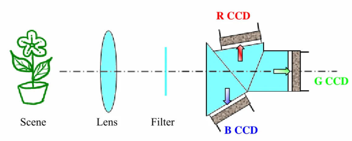
In general, there are two types of images sensing structure for commercial digital camera. One is to use 3 or 4 image sensors to capture image of a scene as shown in Fig. 1. In order to make this structure work, optical paths, optical filters and image sensors for each color channel have to be separated to sense the image of a scene. Once image sensors got R, G and B color information, what we need to reproduce color is just picking up R, G and B color information for each corresponding coordinate without doing color interpolation. It works well! However, it’s a very expensive approach, so that only professional digital cameras use this structure.

Fig. 1. Capture an image by three image sensors structure.

The other one, a single image sensor is used to capture image of a scene as shown in Fig. 2. The structure is much simple so as to reduce camera cost. In order to make this structure work, a color filter with mosaic pattern in front of image sensor to separate color information is necessary. So definitely, the resolution is reduced. To reproduce original color and resolution, interpolation is needed accordingly. At the right hand side of Fig. 2, each small square is representing a pixel. Basically, the pixels beneath color filters are light sensitive cells to respond the intensity of light falling on them. Color filter is aligned to sub-sample color information of a scene. There are many kinds of CFA. In digital camera, Bayer pattern CFA [4] with 3 primary colors R, G and B (as known as Bayer pattern) is widely used. As mention before, this thesis is going to discuss noise reduction method mainly based on this Bayer pattern domain.

R CCD

G CCD

B CCD Lens Filter

Scene

2.2 Bilinear Method

Bilinear is widely used in smoothing edge, typically in the application of re-scaling image size. Also, it can be used in denoising application. The method is described as following equation, ) 1 ( ), , ( * ) 1 )( 1 ( ) 1 , ( * ) 1 ( ) , 1 ( * ) 1 ( ) 1 , 1 ( * ) , ( v u C dv du v u C dv du v u C dv du v u C dudv dv v du u C − − + + − + + − + + + = + +

and illustrated as Fig. 3.

Fig. 3. Reproduced an unknown value C(u+du,v+dv) from its neighboring pixels by using bilinear method.

2.3 Human Visual System

Human Visual System (HVS) is complex and not fully understood yet. It’s difficult to use a mathematical function to represent it. It would be more realistic to get some useful information by experiments. There are two important observations on monochrome image which can be used for noise reduction. The first one is Just Noticeable Difference (JND) which is the minimum amount of stimulus intensity must be changed to cause a noticeable difference in sensory experience.

Ernst Weber (1795~1878), an experimental psychologist in 19th century, observed that the size of the JND threshold is related to initial stimulus magnitude. This relationship, had been simplified as Weber's Law by Gustav Theodor Fechner(1801~1887), can be expressed as

C(u,v) C(u+1,v) C(u+1,v+1) C (u,v+1) du dv C(u+du,v+dv)

Easier to detect noise

Noise is less detectable along this edge

Noise is almost undetectable here It’s difficult to detect noise along this edge

ΔI/I = k. where ΔI represents JND threshold, I represents the initial stimulus intensity and k

stands for the proportional constant. In other words, Weber's Law states that the size of the JND (i.e., ΔI) is a constant which is proportional to the original stimulus value.

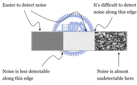
The second one is spatial masking. Natural images contain large changes in luminance, and these changes suppress the ability of the eyes to detect distortions spatially adjacent to them, this is so-called spatial masking. As a result of masking, noises in images are less detectable along strong edges and in highly textured areas, than in smooth areas of the image as illustrated in Fig. 4.

Fig. 4. Spatial Masking effect.

2.4 Bosco-and-Mancuso Filter for Image Denoising

Bosco and Mancuso [1]-[3] invented an adaptive image filter which is used to reduce the amount of noise in images captured by sensors in Bayer pattern format. The concept of this filter acts mainly on smoothing the high spatial frequency components which are hardly

In Bosco and Mancuso’s paper [1] and patent [2],[3], they made use of the Weber’s Law to determine the JND, ΔI, which could be differentiated between intensity I and I+ΔI. Bosco and Mancuso’s HVS model assume that the uniform areas are the ones with details amplitude under JND. Having these considerations in mind they designed an algorithm that can distinguish if the current processed area is uniform area or not. Once the current processed area is not uniform, the algorithm will go to detect how textural the area is and adapts its filtering strength for the noisy pixel.

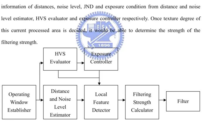
The system block diagram they designed is illustrated in Fig. 5. As mentioned above, the

local feature detector is to compute texture degree of the area. The estimation is based on the

information of distances, noise level, JND and exposure condition from distance and noise level estimator, HVS evaluator and exposure controller respectively. Once texture degree of this current processed area is decided, it would be able to determine the strength of the filtering strength.

Fig. 5. System block diagram of Bosco-and-Mancuso filter.

The algorithm they proposed is to use two different filter masks, depending on which color is current processed pixel. One mask is for green pixels exclusively, the other one is for red/blue pixels, but not operated simultaneously. Fig. 6 is to illustrate those two kinds of operating windows established from Bayer pattern through 2 masks.

Operating Window Establisher Distance and Noise Level Estimator HVS Evaluator Local Feature Detector Filtering Strength Calculator Exposure Controller Filter

G R G1 R G B G2 B G3 B G4 R G0 R G5 B G6 B G7 B G R G8 R G R1 G R2 G R3 G B G B G R4 G R0 G R5 G B G B G R6 G R7 G R8 B1 G B2 G B3 G R G R G B4 G B0 G B5 G R G R G B6 G B7 G B8 G1 G2 G3 G4 G0 G5 G6 G7 G8 R1 R2 R3 R4 R0 R5 R6 R7 R8 1 1 1 1 1 1 1 1 1 × = 1 1 1 1 1 1 1 1 1 × = B1 B2 B3 B4 B0 B5 B6 B7 B8 Bayer pattern Masks Operating windows Fig. 6. Two kinds of operating windows established from Bayer pattern.

Definitely, green operating window is established when current pixel is green. Red and blue operating window will also be established once current pixel is red or blue respectively. The green operating window is different from red and blue, since the green channel has double information comparing with either red or blue channel in Bayer pattern format.

In each case of operating window for red, green and blue, let’s define the current pixel C0 and eight neighboring pixels C1 to C8 respectively. C will also represent for C_i 1 to C8 to describe easier in many cases. So now we have symbol C0 to C8 or C0 and C to stand for i

C0 is the current pixel with noise needed to be filtered. As described in Bosco and Mancuso’s paper and patent, C0 will be filtered and replaced with a weighted average of C1 to

C8. However, how much is the weight of C1 to C8? That will depend on how similar of them to C0. In the design, the higher similarity degree of neighboring pixels, the bigger weight of them to C0. The similarity degree is calculated based on the brightness of current processed pixel and takes into account of the predicted noise level NL of current area as following:

( )

*

[

1

]

*

( )

1, (2) 0

0 t =K Dmax + −K NL t−

NL_{c n n c}

where, Dmax is the maximum distance derived from calculating each distance D of i

neighboring pixel C to C_i 0 and Kn is a parameter to determine the strength of filtering. In the definition, Kn=1 stands for almost flat area since this area could be filtered strongly, and Kn=0 stands for highest texture area as this area could not be filtered too much.

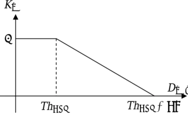
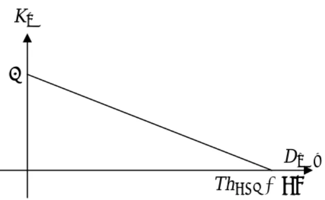
Recall the assumption of uniform area by using Weber’s Law and refers to the Kn definition as above, we can assume the curve of Kn versus Dmax can be drawn as Fig. 7. That’s to say, filter current pixel strongly if Dmax not greater than HVS threshold ThHVS and filter current pixel lighter depending on how noisy the current area is. If Dmax is greater than ThHVS + NL, then the area has to look as a highly texture area without strongly filter needed. However, they used Figs. 8 and 9 instead.

Fig. 7. A candidate of Kn curve.

Kn

Dmax

ThHVS ThHVS + NL 1

Fig. 8. Kn curve for G channel in Bosco and Mancuso’s patents.

Fig. 9. Kn curve for R/B channel in Bosco and Mancuso’s patents.

Kn is the overall filtering strength of current processed area. Although the filtering strength is given, we still need to determine the filtering strength of each neighboring pixel

i

C to target pixel C0. Therefore, in order to evaluate similarity of each neighboring pixel C _i to the target pixel C0, two boundary thresholds refer to Th1 and Th2 are used to stand for most similar and least similar according to following equations:

(

1

)

* , (3) * _{max min} 1 K D K D Th = _n + − _n

(

)

, (4) 2 * 1 * max min max 2 ⎟ ⎠ ⎞ ⎜ ⎝ ⎛ + − + =K D K D D Th _{n n}

where, Dmin is the minimum distance between C0 to C . The value of similarity _i K_i can be determined by Dmax Kn ThHVS + NL 1 Kn NL ThHVS + NL Dmax 1

) 5 ( , for , , if , 0 , if , 1 2 1 1 2 2 2 1 ⎪ ⎪ ⎩ ⎪ ⎪ ⎨ ⎧ < < − − ≥ ≤ = Th D Th Th Th D Th Th D Th D K i i i i i

and Fig. 10 is the illustration for it. At the end, the result of pixel out is expressed as

(

)

[

* 1 *

]

. (6) 8 1 8 1 0

∑

+ − = K C K C PixelOut _{i i i}

Fig. 10. Similarity derived from distance D of neighboring pixel to C_i 0.

2.5 Peak Signal to Noise Ratio

Generally, Peak Signal to Noise Ratio (PSNR) is the most regular way used in the metric of distortion level. It is defined as a ratio between possible maximum power of image intensity and the power of distorted difference in terms of logarithmic decibel scale. In our application, given an original image OM*N and processed image PM*N with dimension of M*N, the PSNR is defined as ) 7 ( , log 10 2 max 10 ⎟⎟ ⎠ ⎞ ⎜ ⎜ ⎝ ⎛ = MSE I PSNR

where, Imax represents for the possible maximum power of image intensity and MSE is defined as

(

) (

)

[

]

) 8 ( . * , , 1 1 2 N M n m O n m P MSE N n M m

∑∑

= = − = i K i D Th1 Th2 1

2.6 Structural Similarity

In many cases, the objective metric of PSNR and MSE could not correlate well with subjective perception. Therefore, Wang [5] developed Structural Similarity (SSIM) which is based on an assumption that HVS is highly sensitive to structural information of a scene, and is defined as

[

( , )

] [

( , )

] [

( , )

]

, (9) ) , (O P l O P α c O P β s O P γ SSIM = ⋅ ⋅

where α, β and γ are the parameters to define the relative importance of the three components. The equation l(O,P), c(O,P) and s(O,P) are defined as

) 10 ( , 2 ) , ( 1 2 2 1 k k P O l P O P O + + + = μ μ μ μ ) 11 ( , 2 ) , ( 2 2 2 2 k k P O c P O P O + + + = σ σ σ σ ) 12 ( , ) , ( 3 3 k k P O s P O OP + + = σ σ σ

Chapter 3

Proposed Image Noise Reduction System

The proposed denoising method would be introduced in this chapter. At the beginning, we would like to have brief description of the image processing on digital camera and the noise category we encountered in Section 3.1. Section 3.2 brings up system block diagram of proposed denoising method. At the end, Section 3.3 explains the detail algorithms.

3.1 Overview of Image Processing on Digital Camera

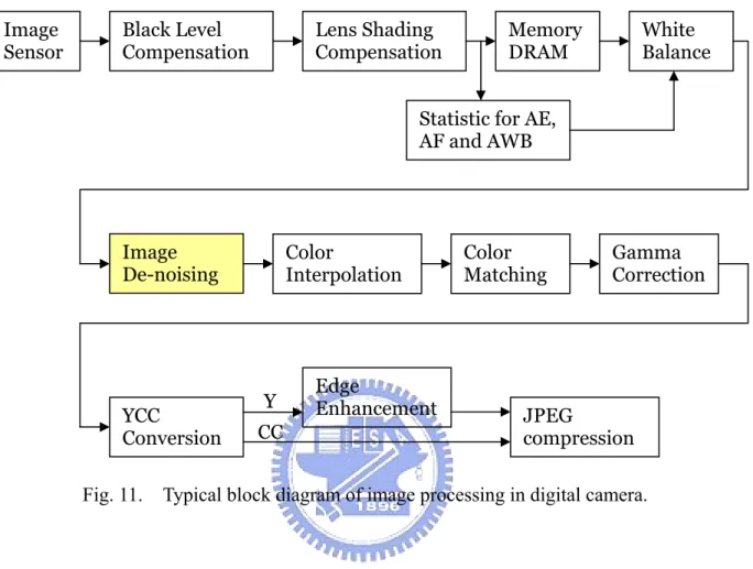
In general, the image processing flow of digital camera is shown as Fig. 11. Once user pressed the shutter button to take an image, the scene in front of camera would be captured by an image sensor, and converted to digital information by analog front end. Normally, black level compensation must be done in front of any processing to calibrate optical black. At the second, lens shading compensation sometimes could be applied. Meanwhile, statistic information for AE, AF and AWB is calculated and stored. And then, save the raw image to memory. What we are going to handle is this raw image. The format of input image is Bayer pattern, and output format of filtered image is Bayer pattern again without any formatting change.

Succeeding to the step of image denoising, color interpolation is normally applied to reproduce the missing color components for each pixel. Since every image sensor has a unique electrical response to light, color matching block is to compensate such kind of deviation. Then, gamma correction is to compensate the non-linearity of display device. YCC conversion block is to transform RGB color domain to YCbCr color domain. Usually, the Y channel will be used to enhance the edge of image. The final step is to perform JPEG compression to output JPEG image.

Fig. 11. Typical block diagram of image processing in digital camera.

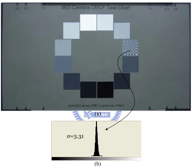
As stated in Chapter 1 that we are interested in random noise. Fig. 12 is an example showing the noisy image captured by a digital camera. Gaussian noise distribution is shown in the histogram as Figs. 12 (b), (d), and (f).

Basically, not only random noise but also fix pattern noise in digital camera need to be handled. However fix pattern noise is much smaller than random noise if the camera made used of CCD sensor to capture image. Therefore, for the noise problem of digital camera, the most headache thing is dealing with Gaussian random noise.

Image Sensor Black Level Compensation Lens Shading Compensation

Statistic for AE, AF and AWB White Balance Memory DRAM Image

De-noising Color Interpolation Color Matching Gamma Correction

YCC Conversion Edge Enhancement _JPEG compression Y CC

σ=3.31

(a)

(b)

Fig. 12. Noise distribution illustration from real camera. (a), (b) Image “OECF” be taken under ISO 100 condition, and its noise distribution; (c), (d) Image “OECF” be taken under ISO 400 condition, and its noise distribution; (e), (f) Image “OECF” be taken under ISO 1600 condition, and its noise distribution.

σ=4.01

σ=6.18 (c)

(d)

3.2 Block Diagram of Proposed Denoising Method

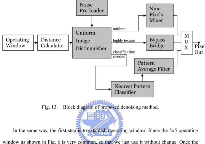
Fig. 13. Block diagram of proposed denoising method.

In the same way, the first step is to establish operating window. Since the 5x5 operating window as shown in Fig. 6 is very common, so that we just use it without change. Once the operating window is determined, a distance calculator is to calculate distance information based on operating window. By feeding the distance information to uniform image distinguisher, the current processed area can be judged as a uniform area, highly texture area or pattern classification needed area based on pre-loaded noise information. Once the processed area has been judged as a uniform area, the succeeding nine pixel mixer will be in charge to output final result and whereas the succeeding bypass bridge will be in charge to output final result while the processed area has been judged as a highly texture area without filtering needed. In the case of processed area is neither a uniform area nor a highly texture area, the succeeding nearest pattern classifier with pattern average filter will be used to output final result. Following Section 3.3 is going to explain the detail about how do they work.

Operating Window Distance Calculator Noise Pre-loader Uniform Image Distinguisher Nearest Pattern Classifier Pattern Average Filter Pixel Out Nine Pixels Mixer Bypass Bridge M U X uniform highly texture classification needed

C1 C2 C3 C4 C0 C5 C6 C7 C8 C1 C2 C3 C4 C0 C5 C6 C7 C8

3.3 Algorithm of Proposed Denoising Method

The same as Chapter 2, the elements C0 ~ C8 of operating window are generically represented for G0 ~ G8, R0 ~ R, and B0 ~ B8 respectively depending on which color is the current pixel to be processed. Fig. 14 is to illustrate the two operating windows which are referred to C0 ~ C8.

(a) (b)

Fig. 14. Two kinds of operating windows. (a) Operating window when current processed color channel is green; (b) Operating window when current processed color channel is red or blue.

Once the operating window is established, the next step is to calculate distance. Distance calculator is going to calculate the distances D of each neighboring pixel to current pixel C_i 0 defined as ) 13 ( 8 2 1 , 0 i , , , . C C D_i = _i − = _L

Also, Dmax and Dmin respectively represent for maximum and minimum distances which can be found once D derived. _i

There are twelve pre-set patterns as shown in Fig. 15. Eqs. (14)-(25) are the equations to calculate the distance of those twelve pre-set patterns to C0 when current processed pixel is green.

(a) (b) (c)

(d) (e) (f)

(g) (h) (i)

(j) (k) (l)

Fig. 15. Pre-set twelve patterns when current processed pixel is green. (a) Horizontal line; (b) Vertical line; (c) Rising line; (d) Falling line; (e) Left-Bottom corner; (f) Bottom-Left corner; (g) Right-Bottom corner; (h) Bottom-Right corner; (i) Right-Top corner; (j) Top-Right corner; (k) Left-Top corner; (l) Top-Left corner.

) 25 ( . ) 24 ( , ) 23 ( , ) 22 ( , ) 21 ( , ) 20 ( , ) 19 ( , ) 18 ( , ) 17 ( , ) 16 ( , ) 15 ( , ) 14 ( , 2 4 2 4 2 1 2 1 3 1 3 1 3 5 3 5 7 5 7 5 7 8 7 8 6 8 6 8 6 4 6 4 6 3 6 3 7 2 7 2 8 1 8 1 5 4 5 4 C C D D D C C D D D C C D D D C C D D D C C D D D C C D D D C C D D D C C D D D C C D D D C C D D D C C D D D C C D D D LT TL TR RT RB BR BL LB RL FL VL HL − + + = − + + = − + + = − + + = − + + = − + + = − + + = − + + = − + + = − + + = − + + = − + + =

When current pixel is red or blue, the pre-set patterns are shown in Fig. 16 and Eqs. (26)-(37) are the equations to calculate distance of those twelve pre-set patterns to C0. The reason of having 2 sets of pattern distance equation is because the index of element is different between green channel and either red or blue channel.

) 37 ( . ) 36 ( , ) 35 ( , ) 34 ( , ) 33 ( , ) 32 ( , ) 31 ( , ) 30 ( , ) 29 ( , ) 28 ( , ) 27 ( , ) 26 ( , 1 4 1 4 1 2 1 2 3 2 3 2 3 5 3 5 8 5 8 5 8 7 8 7 6 7 6 7 6 4 6 4 6 3 6 3 8 1 8 1 7 2 7 2 5 4 5 4 C C D D D C C D D D C C D D D C C D D D C C D D D C C D D D C C D D D C C D D D C C D D D C C D D D C C D D D C C D D D LT TL TR RT RB BR BL LB RL FL VL HL − + + = − + + = − + + = − + + = − + + = − + + = − + + = − + + = − + + = − + + = − + + = − + + =

(a) (b) (c)

(d) (e) (f)

(g) (h) (i)

(j) (k) (l)

Fig. 16. Pre-set twelve patterns when current processed pixel is red or blue. (a) Horizontal line; (b) Vertical line; (c) Rising line; (d) Falling line; (e) Left-Bottom corner; (f) Bottom-Left corner; (g) Right-Bottom corner; (h) Bottom-Right corner; (i) Right-Top corner; (j) Top-Right corner; (k) Left-Top corner; (l) Top-Left corner.

In each case of pattern sets, once the distances of those patterns to C0 are derived,

DmaxPattern and DminPattern which represent for maximum and minimum distances of those patterns to C0 can be found at the same time.

In addition to the distance information, we still need camera noise characteristic which can be obtained by doing noise scanning as a curve shown in Fig. 17.

Fig. 17. Curve fitting for noise characteristic in terms of standard deviation.

Noise pre-loader is doing the job of loading pre-scanned noise level in terms of standard deviation σ which could be obtained by calculating on several flat areas from dark to bright as the small circles shown in Fig. 17. However we would like to use a curve fitted model which has the similar value to the reality noise instead of loading pre-scanned value. Curve fitting

σ

Intensity

Curve Fitting for standard deviation

σmax

max

_σ

yield I

) 38 ( , * 4096 ) ( 1 ) ( _max 2 _ 0 0 max σ σ σ ⎪⎭ ⎪ ⎬ ⎫ ⎪⎩ ⎪ ⎨ ⎧ ⎥ ⎦ ⎤ ⎢ ⎣ ⎡ − − = C Iyield C where, max _σ yield

I is intensity of the flat area which has the maximum standard deviation there as shown in Fig. 17. In the sense, σmax will be different under different ISO speed. Therefore, σmax has to be found for each ISO speed from pre-scanned noise information.

Having both distance information and camera noise characteristic information, we now can distinguish if the current area is uniform or not by using multiple of σ to be the threshold as

( )

C₀ , (39)

m Th_uniform = ∗σ

where, m is a different constant depend on color channel, ISO speed, and also how much captured images like to be filtered. Generally, if DmaxPattern is less than Thuniform, we would consider current area as a uniform image so that the result of output pixel is the average of C0 to C8. On the other hand, if both DmaxPattern and DminPattern are greater than Thuniform, the current area must be a highly texture area without noise reduction needed since the spatial masking of HVS will work fine here. While the Thuniform is between DmaxPattern and DminPattern, the value of

DminPattern will help us to find out which pattern is the nearest pattern. By averaging the element in nearest pattern, the end result of output pixel can be derived. Eq. (40) can help us understand criteria easier.

) 40 ( . f , 3 1 , f , , f , 9 1 min max 3 1 min max 0 max 9 1 ⎪ ⎪ ⎩ ⎪ ⎪ ⎨ ⎧ ≤ ≥ ⋅ ≥ ≥ ≤ ⋅ =

∑

∑

= = uniform Pattern uniform Pattern n n uniform Pattern uniform Pattern uniform Pattern n n Th D and Th D i C Th D and Th D i C Th D i C PixelOut

Chapter 4

Experiments

In this chapter, we would like to discuss the experiment results. The proposed method is implemented in matlab language. There are 148 pieces of test images downloaded from USC, and have been classified to miscellaneous, texture and aerial images. Some of them are monochrome, and some are colored. Those color images have been separated into R, G and B raw information. Hence, 254 pieces of images we have tested in total. Also, the testing images have been classified to miscellaneous, texture and aerial images. Section 4.1 is going to discuss the test results of those images. As for Bayer pattern test images, they were captured by real camera, model: K1003, from market, and will be discussed in Section 4.2.

4.1 Test Results of the Images with Additive Noise:

Tables 1~6 show the noise filtering results for those images with additive Gaussian, Rayleigh, Gamma, Exponential, Uniform and Pepper-and-Salt noises. As shown in the tables, we use 3.125, 7.1875 and 18.75 instead of 5, 10 and 20 of the standard deviation to be the additive random noise. That is because the real camera K1003 we tested has a corresponding relation of ISO 100, 400 and 1600 induce standard deviation σ=3.125, 7.1875 and 18.75 Gaussian noise respectively. It will be more convenient to compare test results of downloaded images and Bayer pattern images by using the same standard deviation.

In order to compare the testing result easier, once the testing result is the maximum value in its own comparing block, the word will be shown in blue. For example, the proposed filter

Table 1.

Proposed SSIM and PSNR compare with other filters for the images with additive Gaussian random noise.

Method

SSIM MSE(12bit) PSNR(dB) SSIM MSE(12bit) PSNR(dB) SSIM MSE(12bit) PSNR(dB)

Original Image

1

0

1

0

1

0

Noisy Image 0.9345215 2635.3187 38.078523 0.7602482 13063.999 31.117336 0.4132095 85827.13 22.940767

Bilinear Filter 0.9458909 8751.3833 35.985395 0.8668262 12459.015 32.961046 0.598386 37903.299 26.78399

BoscoMancuso 0.94303 3211.7889 37.512465 0.8396472 9438.6921 32.709541 0.7069787 25403.612

28.47603

Proposed Filter

0.955219

2369.0048

38.82792 0.877256

7998.7579

33.55646 0.721585

26745.156 28.351483

Method

SSIM MSE(12bit) PSNR(dB) SSIM MSE(12bit) PSNR(dB) SSIM MSE(12bit) PSNR(dB)

Original Image

1

0

1

0

1

0

Noisy Image

0.977307

2692.0342

37.94795

0.9054758 13256.236

31.02415

0.68008 86799.959 22.86681

Bilinear Filter 0.9511116 19645.974 32.04139

0.921281

23277.948 30.299642

0.789722

48656.289

25.76058

BoscoMancuso 0.96658 7787.917 34.328642 0.9108355 20131.951 30.055265 0.7844042 65511.752 25.445342

Proposed Filter0.9710045 3577.3602 36.745723 0.9145903 14094.103 30.941432 0.7851884 67157.284 25.322661

Method

SSIM MSE(12bit) PSNR(dB) SSIM MSE(12bit) PSNR(dB) SSIM MSE(12bit) PSNR(dB)

Original Image

1

0

1

0

1

0

Noisy Image

0.944267

2735.3849

37.87538

0.7844696 13493.13 30.944135 0.4271327 90031.875 22.701765

Bilinear Filter 0.9299304 6294.7093 35.401446

0.859433

9859.6851 32.759052 0.6002676 35215.982 26.819875

BoscoMancuso 0.9407586 4001.8892 36.596138 0.8356556 11066.248 32.068922 0.6667525 29015.028 28.068872

Proposed Filter0.9442624 3093.7263 37.452481 0.8583594 9603.6531

32.76298 0.669239

30138.787

28.11235

Method

SSIM MSE(12bit) PSNR(dB) SSIM MSE(12bit) PSNR(dB) SSIM MSE(12bit) PSNR(dB)

Original Image

1

0

1

0

1

0

Noisy Image 0.9520319 2687.5793

37.96728

0.8167312 13271.122 31.028542 0.5068074 87552.988 22.836447

Bilinear Filter 0.942311 11564.022 34.476077 0.8825132 15198.883 32.00658 0.662792 40591.856 26.454814

BoscoMancuso 0.9501229 5000.5317 36.145748 0.8620461 13545.63 31.611243 0.7193785 39976.797

27.33008

Proposed Filter

0.956829

3013.3638 37.675376

0.883402

10565.505

32.42029 0.725338

41347.076 27.262164

Noisy Image and Filtered

Image Comparing with

Original Image

Adding Gaussian Noise

(σ=3.125)

Adding Gaussian Noise

(σ=7.1875)

Adding Gaussian Noise

(σ=18.75)

Average

Performance

of Misc

images

Average

Performance

of Texture

images

Average

Performance

of Aerial

images

Average

Performance

for above 3

categories

Table 2.

Proposed SSIM and PSNR compare with other filters for the images with additive Rayleigh random noise.

Method

SSIM MSE(12bit) PSNR(dB) SSIM MSE(12bit) PSNR(dB) SSIM MSE(12bit) PSNR(dB)

Original Image

1

0

1

0

1

0

Noisy Image 0.9524053 2108.0467 39.203924 0.8195329 10084.949 32.405071 0.5185017 64174.225 24.362159

Bilinear Filter 0.9544726 8332.0962 36.322186 0.8977145 11236.724 33.56601 0.6872944 32053.961 27.608477

BoscoMancuso 0.9553635 2893.3807 38.059051 0.8745135 8262.0186 33.37031 0.7635932 23782.496

28.78649

Proposed Filter

0.967256

2026.9335

39.56338 0.914593

6627.2968

34.40967 0.776909

25925.48 28.528432

Method

SSIM MSE(12bit) PSNR(dB) SSIM MSE(12bit) PSNR(dB) SSIM MSE(12bit) PSNR(dB)

Original Image

1

0

1

0

1

0

Noisy Image

0.982769

2329.5273

38.61549

0.9254763 11027.233

31.86248

0.7323481 69047.683 23.899324

Bilinear Filter 0.9558581 18219.152 32.364742

0.935453

19827.575 30.958405

0.83327

37271.335

26.81695

BoscoMancuso 0.9713345 7188.3697 34.694235 0.9257176 17597.343 30.623742 0.8211497 53774.549 26.181915

Proposed Filter 0.9752206 3273.8703 37.157302 0.9271713 12606.569 31.447376 0.8156782 62887.65 25.727853

Method

SSIM MSE(12bit) PSNR(dB) SSIM MSE(12bit) PSNR(dB) SSIM MSE(12bit) PSNR(dB)

Original Image

1

0

1

0

1

0

Noisy Image

0.952311

2392.2183

38.49954

0.8129201 11556.016 31.661924 0.481988 75853.428 23.490104

Bilinear Filter 0.934878 5985.4082 35.599208

0.876497

8877.6263

33.18623

0.6493042 30406.011 27.458247

BoscoMancuso 0.9468747 3707.5422 36.90747 0.8533796 9989.9041 32.478467 0.7012338 26447.659

28.45958

Proposed Filter 0.9496021 2841.6673 37.817415 0.873894 8619.5344 33.182683

0.702278

27782.268 28.452171

Method

SSIM MSE(12bit) PSNR(dB) SSIM MSE(12bit) PSNR(dB) SSIM MSE(12bit) PSNR(dB)

Original Image

1

0

1

0

1

0

Noisy Image 0.962495 2276.5974

38.77298

0.8526431 10889.399 31.976493 0.5776126 69691.779 23.917196

Bilinear Filter 0.9484029 10845.552 34.762045 0.9032214 13313.975 32.570213 0.7232894 33243.769 27.294557

BoscoMancuso 0.9578576 4596.4309 36.553585 0.8845369 11949.755 32.157506 0.7619922 34668.235

27.80933

Proposed Filter

0.964026

2714.157 38.179364

0.90522

9284.4666

33.01324 0.764955

38865.133 27.569485

Average

Performance

for above 3

categories

Adding Rayleigh Noise

(σ=18.75)

Average

Performance

of Misc

images

Average

Performance

of Texture

images

Average

Performance

of Aerial

images

Noisy Image and Filtered

Image Comparing with

Original Image

Adding Rayleigh Noise

(σ=3.125)

Adding Rayleigh Noise

(σ=7.1875)

Table 3.

Proposed SSIM and PSNR compare with other filters for the images with additive Gamma random noise.

Method

SSIM MSE(12bit) PSNR(dB) SSIM MSE(12bit) PSNR(dB) SSIM MSE(12bit) PSNR(dB)

Original Image

1

0

1

0

1

0

Noisy Image 0.9468771 3923.0955 36.601812 0.8055776 18585.55 29.843401 0.5023506 108338.14 22.119836

Bilinear Filter 0.9526165 9373.675 35.066067 0.8889569 17880.457 30.807949 0.6684268 71676.381 24.061314

BoscoMancuso 0.9517971 4601.662 36.09254 0.8661901 15798.758 30.695568 0.7468097 62465.894

24.86763

Proposed Filter

0.962456

3819.0176

36.86021 0.901636

15091.346

31.05836 0.750736

71338.921 24.371313

Method

SSIM MSE(12bit) PSNR(dB) SSIM MSE(12bit) PSNR(dB) SSIM MSE(12bit) PSNR(dB)

Original Image

1

0

1

0

1

0

Noisy Image

0.980834

4048.3634

36.45442

0.9202432 18567.251 29.779769 0.7246066 104345.14 22.168423

Bilinear Filter 0.9587397 16716.207 32.455294

0.939066

19828.859

30.53282 0.834452

53357.365

25.34136

BoscoMancuso 0.971281 7982.279 34.189189 0.9263285 21341.208 29.764013 0.8317934 67193.132 25.040787

Proposed Filter0.9739903 4980.7568 35.473742 0.9238756 20166.031 29.720223 0.8120095 99742.349 23.943844

Method

SSIM MSE(12bit) PSNR(dB) SSIM MSE(12bit) PSNR(dB) SSIM MSE(12bit) PSNR(dB)

Original Image

1

0

1

0

1

0

Noisy Image

0.951178

3053.7849

37.50087

0.810479 14725.317 30.660279 0.4845545 94198.712 22.559213

Bilinear Filter 0.937584 6051.2398 35.561203

0.880459

10539.637

32.63553

0.6566235 44080.417 26.146491

BoscoMancuso 0.9476738 4107.58 36.572273 0.8571346 12033.662 31.883421

0.714269

38748.237

27.29767

Proposed Filter 0.949818 3454.768 37.094764 0.8747839 11548.832 32.264883 0.7111025 42946.461 27.181801

Method

SSIM MSE(12bit) PSNR(dB) SSIM MSE(12bit) PSNR(dB) SSIM MSE(12bit) PSNR(dB)

Original Image

1

0

1

0

1

0

Noisy Image 0.9596297 3675.0813

36.85237

0.8454333 17292.706 30.094483 0.5705039 102294 22.282491

Bilinear Filter 0.9496467 10713.707 34.360854

0.902827

16082.984

31.32543

0.7198342 56371.387 25.183055

BoscoMancuso 0.9569173 5563.8403 35.618001 0.8832178 16391.209

30.781

0.764291

56135.754

25.73536

Proposed Filter

0.962088

4084.8475 36.476239 0.9000984 15602.07 31.014488 0.7579495 71342.577 25.165652

Noisy Image and Filtered

Image Comparing with

Original Image

Adding Gamma Noise

(σ=3.125)

Adding Gamma Noise

(σ=7.1875)

Adding Gamma Noise

(σ=18.75)

Average

Performance

of Misc

images

Average

Performance

of Texture

images

Average

Performance

of Aerial

images

Average

Performance

for above 3

categories

Table 4.

Proposed SSIM and PSNR compare with other filters for the images with additive Exponential random noise.

Method

SSIM MSE(12bit) PSNR(dB) SSIM MSE(12bit) PSNR(dB) SSIM MSE(12bit) PSNR(dB)

Original Image

1

0

1

0

1

0

Noisy Image 0.9538932 1916.0539 39.703041 0.8278349 9171.7644 32.892586 0.5404806 55881.464 25.003254

Bilinear Filter 0.9542979 8318.3242 36.413495 0.8999395 10783.027 33.927708 0.7056303 27208.719 28.445277

BoscoMancuso 0.9554814 2767.8087 38.328801 0.8711072 7869.327 33.648945 0.7638481 21312.695 29.324212

Proposed Filter

0.964009

1934.0347

39.82872 0.903121

6360.8482

34.60461 0.78714

21304.67

29.45893

Method

SSIM MSE(12bit) PSNR(dB) SSIM MSE(12bit) PSNR(dB) SSIM MSE(12bit) PSNR(dB)

Original Image

1

0

1

0

1

0

Noisy Image

0.983237

2137.9798

39.01697

0.9282737 10101.145

32.27136

0.7469824 60810.245 24.473434

Bilinear Filter 0.95507 18765.966 32.283742

0.934426

20676.762 30.896156

0.838341

36237.881

27.04295

BoscoMancuso 0.971111 7228.5954 34.70439 0.9233719 17785.997

30.61 0.8138668 55504.168 26.107744

Proposed Filter 0.9748681 3110.5723 37.401785 0.9235726 12031.845 31.592684 0.815686 58407.968 26.017606

Method

SSIM MSE(12bit) PSNR(dB) SSIM MSE(12bit) PSNR(dB) SSIM MSE(12bit) PSNR(dB)

Original Image

1

0

1

0

1

0

Noisy Image

0.952762

2328.7978

38.64061

0.8182523 11233.554 31.806479 0.5019272 69021.956 23.901791

Bilinear Filter 0.9340914 6044.9248 35.569447

0.876264

8876.268

33.19371

0.663491 27849.38 27.845443

BoscoMancuso 0.9458779 3711.0621 36.897107 0.8462719 10219.802 32.352077 0.6965737 26525.128 28.454309

Proposed Filter 0.9458406 2879.239 37.741935 0.8583505 9119.3632 32.819789

0.705502

26401.613

28.69633

Method

SSIM MSE(12bit) PSNR(dB) SSIM MSE(12bit) PSNR(dB) SSIM MSE(12bit) PSNR(dB)

Original Image

1

0

1

0

1

0

Noisy Image

0.963298

2127.6105

39.12021

0.8581203 10168.821 32.323475 0.5964634 61904.555 24.459493

Bilinear Filter 0.9478198 11043.072 34.755561

0.903543

13445.352 32.672525 0.7358207 30431.994 27.77789

BoscoMancuso 0.9574901 4569.1554 36.643433 0.8802503 11958.375 32.203674 0.7580962 34447.33 27.962088

Proposed Filter 0.9615725 2641.282 38.324145 0.8950146 9170.6856

33.0057 0.769443

35371.417

28.05762

Noisy Image and Filtered

Image Comparing with

Original Image

Adding Exponential Noise

(σ=3.125)

Adding Exponential Noise

(σ=7.1875)

Adding Exponential Noise

(σ=18.75)

Average

Performance

of Misc

images

Average

Performance

of Texture

images

Average

Performance

of Aerial

images

Average

Performance

for above 3

categories

Table 5.

Proposed SSIM and PSNR compare with other filters for the images with additive Uniform random noise.

Method

SSIM MSE(12bit) PSNR(dB) SSIM MSE(12bit) PSNR(dB) SSIM MSE(12bit) PSNR(dB)

Original Image

1

0

1

0

1

0

Noisy Image 0.9466853 3924.5979 36.604222 0.8036968 18604.176 29.836767 0.4964588 109637.05 22.066244

Bilinear Filter 0.9526122 9375.4442 35.066494 0.8884286 17887.981 30.80699 0.6631888 72237.356 24.021099

BoscoMancuso 0.950285 4613.0272 36.065946 0.8594214 15968.515 30.635285 0.7373354 63346.948

24.77497

Proposed Filter

0.963068

3811.8075

36.87933 0.90416

15010.803

31.07655 0.748584

71594.946 24.33555

Method

SSIM MSE(12bit) PSNR(dB) SSIM MSE(12bit) PSNR(dB) SSIM MSE(12bit) PSNR(dB)

Original Image

1

0

1

0

1

0

Noisy Image

0.980778

4049.9905

36.45284

0.9196255 18622.458 29.766729 0.7200411 105759.46 22.105561

Bilinear Filter 0.9587221 16716.134 32.455076

0.938936

19847.905

30.52765 0.831692

53892.557

25.28707

BoscoMancuso 0.9713056 7983.0211 34.189932 0.9267439 21345.365 29.766276 0.8291931 67717.684 24.973077

Proposed Filter 0.9740785 4979.8103 35.475321 0.9247218 20171.318 29.727771 0.8110182 100198.21 23.91431

Method

SSIM MSE(12bit) PSNR(dB) SSIM MSE(12bit) PSNR(dB) SSIM MSE(12bit) PSNR(dB)

Original Image

1

0

1

0

1

0

Noisy Image

0.951126

3050.9628

37.5055

0.8089396 14727.829 30.659513 0.4789032 95197.107 22.513315

Bilinear Filter 0.9375922 6051.0579 35.563036

0.880124

10542.482

32.63464

0.6525323 44444.054 26.105319

BoscoMancuso 0.9474257 4111.8302 36.562772 0.8545456 12118.549 31.832587 0.7059513 39464.875 27.148317

Proposed Filter 0.9504938 3440.4087 37.120414 0.8776947 11453.156 32.33459

0.709854

43117.236

27.15497

Method

SSIM MSE(12bit) PSNR(dB) SSIM MSE(12bit) PSNR(dB) SSIM MSE(12bit) PSNR(dB)

Original Image

1

0

1

0

1

0

Noisy Image 0.9595298 3675.1837

36.85419

0.8440873 17318.155 30.08767 0.5651344 103531.2 22.228373

Bilinear Filter 0.9496422 10714.212 34.361535

0.902496

16092.789

31.32309

0.7158043 56857.989 25.137828

BoscoMancuso 0.9563388 5569.2928 35.606217 0.880237 16477.477 30.744716

0.757493

56843.169

25.63212

Proposed Filter

0.962547

4077.3421 36.491687 0.9021921 15545.092 31.046305 0.7564855 71636.796 25.134943

Noisy Image and Filtered

Image Comparing with

Original Image

Adding Uniform Noise

(σ=3.125)

Adding Uniform Noise

(σ=7.1875)

Adding Uniform Noise

(σ=18.75)

Average

Performance

of Misc

images

Average

Performance

of Texture

images

Average

Performance

of Aerial

images

Average

Performance

for above 3

categories

Table 6.

Proposed SSIM and PSNR compare with other filters for the images with additive Pepper-and-Salt random noise.

Method

SSIM MSE(12bit) PSNR(dB) SSIM MSE(12bit) PSNR(dB)

Original Image

1

0

1

0

Noisy Image 0.6280432 106620.26 22.010358 0.6280432 106620.26 22.010358

Bilinear Filter

0.71665

44444.204

26.06897

0.7166504 44444.204 26.068965

BoscoMancuso 0.7002945 59926.768 24.5426 0.7002945 59926.768 24.5426

Proposed Filter 0.6122379 107459.05 21.974556

0.937776

15220.672

30.73973

Method

SSIM MSE(12bit) PSNR(dB)

SSIMMSE(12bit) PSNR(dB)

Original Image

1

0

1

0

Noisy Image 0.7812048 103674.45 22.1105 0.7812048 103674.45 22.1105

Bilinear Filter

0.82964

54786.666

25.25988

0.8296402 54786.666 25.259881

BoscoMancuso 0.8118458 70802.997 23.869474 0.8118458 70802.997 23.869474

Proposed Filter 0.7686513 105006.78 22.053915

0.948625

23049.538

29.30574

Method

SSIM MSE(12bit) PSNR(dB)

SSIMMSE(12bit) PSNR(dB)

Original Image

1

0

1

0

Noisy Image 0.6385427 98627.618 22.32257 0.6385427 98627.618 22.32257

Bilinear Filter

0.71295

38241.843

26.46561

0.7129502 38241.843 26.46561

BoscoMancuso 0.6858612 58501.829 24.594154 0.6858612 58501.829 24.594154

Proposed Filter 0.6100298 100111.22 22.256986

0.915285

13365.4

31.08356

Method

SSIMMSE(12bit) PSNR(dB)

SSIMMSE(12bit) PSNR(dB)

Original Image

1

0

1

0

Noisy Image 0.6825969 102974.11 22.147809 0.6825969 102974.11 22.147809

Bilinear Filter

0.75308

45824.237

25.93149

0.7530802 45824.237 25.931485

BoscoMancuso 0.7326672 63077.198 24.335409 0.7326672 63077.198 24.335409

Proposed Filter 0.6636397 104192.35 22.095152

0.933895

17211.87

30.37634

Average

Performance

of Aerial

images

Average

Performance

for above 3

categories

Noisy Image and Filtered

Image Comparing with

Original Image

Adding Pepper-and-Salt Noise

ISO 100 and ISO 400

(didn't handle singular point)

Average

Performance

of Misc

images

Average

Performance

of Texture

images

Adding Pepper-and-Salt Noise

ISO 1600

In general, the proposed filter has better SSIM and PSNR than Bosco-and-Mancuso filter as the test results shown in the row named “Average Performance for above 3 Categories” in Tables 1~6. However, there are some special cases such as noisy images have better SSIM and PSNR than filtered images as the results shown in the row named “Average Performance of Texture Images” and “Average Performance of Aerial Images” in Tables 1~5, bilinear filter has better SSIM than proposed filter as the results shown in the row named “Average Performance of Texture Images” and “ Average Performance of Aerial Images” in Tables 1~5, proposed filter has worse PSNR even if it has better SSIM than others as the results shown in the row named “Average Performance of Misc Images” in Tables 1, 2, 3, and 5, proposed filter has worst SSIM on texture images under high Gamma and Uniform noise condition as the results shown in the row named “Average Performance of Texture Images” in Tables 3 and 5, proposed filter is not able to filter out Pepper-and-Salt noise under ISO 100 and 400 conditions as the results shown in the column named “Adding Pepper-and-Salt Noise for ISO 100 and ISO 400 (didn't handle singular point)” in Table 6, and proposed filter performs not badly in each kind of test patterns as shown in Tables 9~14. The phenomena mentioned as above have been brought up for case study as following:

Case 1: Noisy images have better SSIM and PSNR than filtered images:

The reason of noisy images have better SSIM and PSNR than filtered images is because original images themselves have had much random noise scattered on themselves already without additive noise. We have chosen a worst case for an example as shown in Fig. 18. The original image “1.3.08-Water” is shown in Fig. 18(a) and its 400% enlarged sub-image is shown in Fig. 18(b). By calculating a block in the sub-image, that σ=7 random noise at flat area has been found as shown in Fig. 18(b). No wonder that Fig. 18(c) which is the image “1.3.08-Water” with additive σ=3.125 Gaussian noise looks very similar to the original image by our eyes’ perception. As for filtered images shown in Figs. 18(d)-(f), not only additive

noise have been filtered, but also a lot of original images have been handled as noisy signals, so that filtered images are not so similar as noisy images to the original images. In the category of aerial images, it has the same situation as texture images so that noisy images have better SSIM and PSNR than filtered images. Fig. 19 is another example which is an aerial image to explain this phenomenon, and the situation of this image is totally the same as Fig. 18. So it could be understood by consulting the above analysis for this example.

Case 2: Bilinear filter has better SSIM than proposed filter: In our evaluation, the bilinear filter is implemented as

) 41 ( . 2 4 ) ( 0 5 4 7 2 C C C _C C PixelOut + + + + =

Therefore the filtering strength of bilinear filter is less than Bosco-and-Mancuso filter and proposed filter, when Bosco and Mancuso’s algorithm and proposed algorithm handle the current image block as a uniform area.

The worst case happen on this case is still the image named “1.3.08-Water”. So we use 2nd worst case, image “1.5.06-BrickWall”, for an example as shown in Fig. 20. The original image is shown in Fig. 20(a) and its 400% enlarged sub-image is shown in Fig. 20(b). It’s not difficult to observe that the original image is very noisy already. The standard deviation of each brick is around 6.5. Fig. 20(c) shows the image “1.5.06-BrickWall” with additional σ=7.1875 Gaussian noise. Also, the filtered images have been shown in Figs. 20(d)-(f). From subjective observation, we would say, the image filtered by bilinear filter as shown in Fig. 20(d) has the highest similarity to the original images, the same as objective metric. It’s a reasonable result since original image is very noisy already, so that denoising filter with less

(a) (b)

(c) (d)

(e) (f)

Fig. 18. An example illustrated that noisy texture image has better SSIM and PSNR than filtered images. (a) Original image “1.3.08-Water”; (b) 400% enlarged; (c) Adding σ=3.125 Gaussian noise; (d) Filtered by Bilinear filter; (e) Filtered by Bosco-and-Mancuso filter; (f) Filtered by Proposed filter.

(a) (b)

(c) (d)

(a) (b)

(c) (d)

(e) (f)

Fig. 20. An example illustrated that bilinear filter has better SSIM than proposed filter. (a) Original image “1.5.06-BrickWall”; (b) 400% enlarged; (c) Adding σ=7.1875 Gaussian noise; (d) Filtered by Bilinear filter; (e) Filtered by Bosco-and-Mancuso filter; (f) Filtered by Proposed filter.

Case 3: Proposed filter has worse PSNR even if it has better SSIM than others:

Basically, case 3 illustrates the reason why Wang developed SSIM for image assessment [5]-[7]. In some cases, images look very un-acceptable even if those images have the same PSNR as acceptable images [5]-[8]. So in general, case 3 is not a special case needed to bring up for a discussion, since proposed filter keep more structural information such as edge information.

However, when we surveyed the worst case of images, there is a drawback found in the proposed algorithm. That is proposed algorithm will yield contour seriously if the image has been added too much random noise such as σ=18.75 shown in Fig. 21. The original image “4.1.08-JellybeansG” is shown in Fig. 21(a) and its 400% enlarged sub-image is shown in Fig. 21(b). Besides, the image with additive σ=18.75 Gaussian noise is shown in Fig. 21(c) and its 400% enlarged sub-image is shown in Fig. 21(d). The reason to yield contour under big noise condition is because current processed pixel will handle the neighboring pixels as noisy pixel when pixel signal is under transient position either from bright to dark or dark to bright, so that current processed pixel will chose a nearest pattern to be its filtering elements instead of applying spatial masking on those transient pixels. By choosing nearest pattern to filter noisy pixel, the value of processed pixel will close to the nearest pattern. In the case of transient pixels changed slowly so that they consist of many pixels. Then the value of one side of them will join bright area and whereas the other side of them will join dark area. Therefore contour effect is enhanced as shown in Figs. 21(i)-(j). Comparing with Figs. 21(e)-(h) which are the images outputted from bilinear filter and Bosco-and-Mancuso filter respectively, they have no this kind of contour problem. This is the case that the proposed algorithm doesn’t like to see, and unable to filter this kind of transient pixels well under big noise condition. Nevertheless,

22, 23 and Table 7. Figs. 22(a) and 23(a) show the image “4.1.08-JellybeansG” with additive Gaussian noise and that Figs. 22(b) and 23(b) show their 400% enlarged sub-image. Both two sets of Figs. 22(c)-(e) and 23(c)-(e) show the images outputted from bilinear filter, Bosco-and-Mancuso filter, and proposed filter respectively. As subjective observation, bilinear filter looks too blue and whereas proposed filter has strongest edge information. Table 7 is also to illustrate that proposed filter has best filtering result on flat area.

(a) (b)

(c) (d)

Fig. 21. Proposed filter has worse PSNR even if it has better SSIM than others. (a) Original image “4.1.08-JellybeansG”; (b) 400% enlarged; (c) adding σ=18.75 Gaussian noise; (d) 400% enlarged; (e) Filtered by Bilinear filter; (f) 400% enlarged; (g) Filtered by Bosco-and-Mancuso filter; (h) 400% enlarged; (i) Filtered by proposed filter; (j) 400% enlarged.

(e) (f)

(a) (b)

(c) (d)

(e)

Fig. 22. Proposed filter has better filtering result under σ=7.1875 Gaussian noise. (a) Adding σ=7.1875 Gaussian noise; (b) 400% enlarged; (c) Filtered by Bilinear filter; (d) Filtered by Bosco-and-Mancuso filter; (e) Filtered by proposed filter.

(a) (b)