真實處理器之高能源效率任務內動態電壓調整策略

國

立

交

通

大

學

資訊科學系

碩

士

論

文

真實處理器之高能源效率任務內動態電壓調整策略

Energy Efficient Stochastic Intra-Task Dynamic Voltage Scaling

for Realistic CPUs

研 究 生：楊建中

指導教授：王國禎 博士

真實處理器之高能源效率任務內動態電壓調整策略

Energy Efficient Stochastic Intra-Task Dynamic Voltage Scaling

for Realistic CPUs

研 究 生：楊建中 Student：Chien-Chung Yang

指導教授：王國禎 Advisor：Kuochen Wang

國 立 交 通 大 學

資 訊 科 學 系

碩 士 論 文

Submitted to Department of Computer and Information Science College of Electrical Engineering and Computer Science

National Chiao Tung University in Partial Fulfillment of the Requirements

for the Degree of Master

in

Computer and Information Science June 2005

Hsinchu, Taiwan, Republic of China

i

真實處理器之高能源效率任務內

動態電壓調整策略

學生：楊建中 指導教授：王國禎 博士

國立交通大學資訊科學系

摘 要

這幾年來，個人隨身助理與手機等手持裝置需要運算能力強大的

處理器來快速地處理各種多媒體應用。然而越快速的處理器所消耗的

能源也越高。如果將處理器一直維持在最高速度來執行所有的工作，

會造成能源的浪費。動態電壓調整演算法可以依據處理器的實際工作

量，動態調整其頻率與電壓來達到省電的目的，而一個好的演算法必

須也能滿足即時性工作的時間限制。本篇論文有兩個主要貢獻：第

一，相對於 PACE [2]複雜的推導，在任務內動態電壓調整模型下，

我們利用朗冠吉係數法很簡潔地導出消耗最少能源的最佳速度排

程。第二，PACE 假設處理器模型是理想的，也就是說這種處理器能

支援各種的頻率以及相對應的電壓。我們稱這種處理器為理想處理

器。事實上，一般處理器只能提供有限的頻率及電壓組合，相對於理

想處理器，我們稱這種處理器為真實處理器。因為能源消耗並不是簡

單的頻率函數，將原本的非線性規劃問題轉換成多重選擇背包問題是

比較合理的。我們利用動態規劃法導出在真實處理器上消耗最少能源

的最佳速度排程。分析結果顯示，相較於 PACE，我們的演算法平均

節省了三倍真實處理器的能源。

關鍵詞：能源效益，任務內動態電壓調整，可攜式系統，即時。

iii

Energy Efficient Stochastic Intra-Task Dynamic

Voltage Scaling for Realistic CPUs

Student：Chien-Chung Yang Advisor：Dr. Kuochen Wang

Department of Computer and Information Science National Chiao Tung University

Abstract

In recent years, hand-held devices such as personal digital assistants (PDAs) and cell phones require powerful CPUs to handle a variety of multimedia applications as fast as possible. However, the faster the CPU speed, the higher the CPU energy consumption. It is not energy efficient to run a CPU in full speed all the time for all kinds of tasks. A dynamic voltage scaling (DVS) algorithm can adjust CPU frequency/voltage dynamically depending on CPU workloads to save energy, and a graceful DVS algorithm must meet the time constraint of each real time task. There are two main contributions in this thesis. First, unlike the tedious derivation in PACE [2], we have derived an optimal speed schedule with minimal energy consumption in the intra-task DVS model in an elegantly way by using the Lagrange multiplier procedure. Secondly, the CPU model assumed in PACE is ideal, meaning that the CPU supports all kinds of frequencies and corresponding voltages. We call such CPUs as ideal CPUs. In reality, CPUs only support a limited set of frequency/voltage levels, and we call this kind of CPUs as realistic CPUs in contrast to ideal CPUs. Since energy consumption is not a simple function of frequency, it is more reasonable to transform the original nonlinear programming problem to a

multiple-choice knapsack problem (MKP) [35]. We use dynamic programming to

consumption. Analysis results have shown that the energy saving of the proposed OSRC is three times in average better than that of PACE in realistic CPUs.

Keywords：energy efficient, intra-task dynamic voltage scaling, portable system,

v

Acknowledgements

Many people have helped me with this thesis. I deeply appreciate my thesis advisor, Dr. Kuochen Wang, for his intensive advice and instruction. I would like to thank all the classmates in Mobile Computing and Broadband Networking Laboratory for their invaluable assistance and suggestions. This work was supported by the NCTU EECS-MediaTek Research Center under Grant Q583.

Contents

Abstract (in Chinese) i

Abstract (in English) iii

Acknowledgements v

Contents vi

List of Figures viii

List of Tables ix

1. Introduction...1

2. Related Work...4

2.1 Dynamic Voltage Scaling...4

2.2 Inter-task DVS ...5

2.3 Intra-task DVS ...5

3. Optimal Speed Schedule for Ideal CPUs ...7

3.1 Stochastic Intra-task DVS...7

3.2 Simplifying the Derivation in PACE by Lagrange Multiplier Procedure...8

4. Proposed Optimal Schedule in Realistic CPUs (OSRC) ...12

4.1 The Problem of the PACE in Realistic CPUs ...12 4.2 PACE Approach: Rounding the Frequencies Obtain from PACE to the

vii

Nearest Available Frequencies...14

4.3 OSRC Approach...15

5. Evaluation and Discussion ...20

5.1 Simulation Model...20

5.2 Impact of CPU levels ...21

5.3 Impact of BCEC/WCEC (α) ratio...23

6. Conclusions and Future Work ...27

6.1 Concluding Remarks...27

6.2 Future Work ...28

List of Figures

Fig. 1. OSRC procedure...17 Fig. 2. The recursion graph to solve Task 1. ...19 Fig. 3. The impact of CPU levels on expected energy consumption in Intel

PXA255...22 Fig. 4. The impact of CPU levels on expected energy consumption in Intel

PXA270...23 Fig. 5. The impact of

α

(

α

α

(

α

α

(

α

α

ix

List of Tables

Table 1：Power consumption specification for Intel PXA255. ...13

Table 2：Power consumption specification for Intel PXA270. ...13

Table 3：Specifications of two example tasks ...14

Table 4：Simulation parameters...21

Chapter 1

Introduction

Hand-held devices are powered by batteries for mobility needs. In each battery operated system, we need effective power management to use energy efficiently to extend battery life. Such battery operated systems often build in embedded systems for special purposes. Different purposes need different power management schemes. In communication embedded systems, like cell phones, they often consume a lot of energy in radio interfaces. If the radio interface still works in full power when there is no data communication, it wastes energy. In wireless sensor embedded systems, they often become active once in a week, or even once a month. To save energy, the basic method is to change a sensor node from active to sleep state when it is not used. In high-speed embedded systems, like multimedia personal digital assistants (PDAs), they use high-speed CPUs (in contrast to other embedded systems) to handle multimedia applications.

Manufacturers usually make hand-held devices, like multimedia PDAs or cell phones more powerful by using faster CPUs to handle complex functions. But the faster the CPU is, the more energy it consumes. Note that CPU frequency is directly proportional to the voltage applied, and energy is proportional to the square of the voltage applied [1]. The basic idea to save energy by adjusting CPU frequency is that we don’t need a high CPU frequency to handle simple jobs, like text editing which requires lower CPU frequency than that for media playing. Even in the media playing,

2

a device only needs to satisfy the user’s requirement by using a proper CPU frequency. It has been shown that decreasing the CPU frequency linearly, the energy consumption can be reduced quadratically. Of course, such CPUs must support frequency and voltage scaling, like Intel Xcale, Transmeta Cursoe and Intel

Pentium-M.

We can not decrease CPU speed by reducing frequency and voltage without considering performance. System performance must be considered as well. The question here is how to choose a proper CPU speed that meets the system performance requirement. In the OS level point of view, giving a task with deadline d, and worst case execution cycles (WCEC) C, we can determine an optimal static speed,

C/d, such that the task can be completed before deadline d [6]. A real time system can

be classified into hard and soft. In a hard real time system, all its tasks must finish before their deadlines; otherwise the system will crash. In a soft real time system, it allows some proportion of tasks missing their deadlines and the system still works. Both kinds of real time systems need to know a task’s workload and deadline, and the OS scheduler arranges each task to run to meet its deadline. Often a task’s CPU requirement is assigned off-line, which is usually overestimated to avoid deadline miss. As a result when tasks complete early, CPU idle time (called slack time) occurs. A DVS algorithm tries to adjust the CPU frequency of a system to reduce the CPU slack time and the system still meet hard or soft real time constraint for a task. However, it is hard to predict a task’s actual workload before the task finishes due to conditional branches or loops. In other words, we never know an optimal DVS solution before tasks are completed. Because of the indefinite task’s workload, it is not energy efficient if the DVS algorithm uses a static frequency for each task [13]. In summary, the main issue of the DVS is how to adjust CPU frequency and voltage dynamically and still guarantee system performance.

In this thesis, we address the energy efficient intra-task voltage scaling for ideal CPUs and realistic CPUs under the stochastic model, respectively. For realistic CPUs, we propose an energy efficient intra-task DVS algorithm for hard real time systems. The rest of the thesis is organized as follows. Chapter 2 gives background and related work. Chapter 3 derives an optimal energy efficient intra-task DVS algorithm for ideal CPUs in an elegant way. In Chapter 4, we formulate the DVS problem for realistic CPUs as MKP and propose an energy efficient algorithm based on dynamic programming. Finally, conclusion remarks and future work are outlined in Chapter 5.

4

Chapter 2

Related Work

2.1 Dynamic Voltage Scaling

DVS is a feature that a system can adjust device voltage dynamically to save energy. Many notebooks provide simple but inconvenient voltage scaling methods. For example, in Toshiba Satellite serial laptops [12], users can select different power saving modes manually. Previous researches focused on DVS algorithms that were based on CPU utilization to increase or decrease CPU frequency to save energy dynamically [9][20]. But these algorithms may fail in real time systems because the deadlines of the tasks were not considered, and it is not correct to assume that the future CPU utilization always is same as the current one.

F. Yao et al. [30] first proposed a simple model of job scheduling in real time systems, which was further enhanced by B. Mochocki et al. [25] with consideration of the voltage transition overhead. Ishihara and Yasuura [21] formulated the voltage scheduling problem in a processor, which can use only a small number of discrete voltages, as an integer linear programming (ILP) problem. Various voltage scheduling algorithms have been proposed for real time distributed systems enabled with discrete voltage scaling [22][25][26][27][28], which were also formulated as an ILP problem. Andrei et al. [27] proved that the discrete voltage selection formulated as an ILP problem is indeed NP-hard, no optimal solution can be found in polynomial time.

The real time DVS algorithms can be classified into inter-task and intra-task based on the granularity at which the voltage scaling is performed [34]. In intra-task DVS algorithms, the CPU frequency is changed dynamically during running a task, while inter-task DVS algorithms keep it static in a task and change it across tasks.

2.2 Inter-task DVS

Inter-task DVS algorithms focus on how to assign a proper CPU frequency when a task is dispatched by the scheduler. We often apply earliest deadline first (EDF) schedulers in periodical real time systems, and the CPU frequency and voltage are constant during running this task. Pillai and Shin [8] proposed a look-ahead technique to determine future computation need and defer task execution, so the current running task always works under the lowest CPU frequency as possible. Aydin and Melhem [13] used a dynamic reclaiming algorithm and an aggressive speed adjustment procedure in the EDF scheduler. The reclaiming algorithm uses a greedy method to compute earliness of a task, and the aggressive speed adjustment procedure

determines the maximum amount of additional CPU time that can be assigned to this task.

2.3 Intra-task DVS

Intra-task DVS algorithms adjust the CPU frequency during running a task by its deadline and remaining execution cycles. Shin et al. [10] first proposed an intra-task DVS for hard real time applications by using remaining WCEC-based speed

6

assignment, and voltage scaling decisions are made at compile time to reduce runtime overhead. But it is not energy efficient if we frequently change the CPU speed.

AbouGhazaleh et al. [6] applied a collaborative operating system and compiler algorithm to reduce voltage scaling overhead. The compiler inserts the information of WCEC to the source code, and the timing of changing CPU frequency is control by the operating system, called power management point. The above two DVS

algorithms have a common property that tasks execute at high frequency first and decelerate [5][14]; it wastes energy if tasks poorly finish in WCET. Shin and Kim [18] used the average case execution path (ACEP) as a reference path to decrease CPU frequency in the beginning of the task running, but Seo et al. [14] claimed that an ACEP-based algorithm does not always achieve minimum average energy

consumption and proposed an optimal-case execution path based on probability. But this algorithm only supports the control flow graphs which each of branches only has two successors. Although the program analysis based on intra-task DVS algorithms does not require OS modification [10][18], the shortcoming is that if can not

collaborate with the other inter-task DVS algorithms. This is because during compile time, the frequency/ voltage scaling code is inserted and the CPU frequency is static. Gruain [5] first proposed a stochastic model for intra-task DVS algorithms, which is better than reclaim-based intra-task ones [6][10][18]. A reclaim-based intra-task DVS is that the CPU frequency is calculated dynamically during running a task. Lorch and Smith [2] proved that the optimal speed is inverse proportion to the cube root of the tail probability in Gruain’s stochastic model, but this optimal speed scheduler does not work energy efficiently in real world if the CPU only support a limited set of

Chapter 3

Optimal Speed Schedule for Ideal

CPUs

We discuss an optimal speed schedule with minimal energy consumption in ideal CPUs. The clock frequency is assumed linearly related to the supply voltage. For any CPU frequency changes, the supported voltage can change as well. Although Lorch and Smith [2] have derived such an optimal schedule, called PACE, their proof is tedious and did not take the restriction of a limited set of supported frequency/voltage levels and the actual power consumption of a CPU into account. Therefore, we first formulate the optimal schedule problem as a constrained nonlinear programming problem, and derive an optimal speed schedule for ideal CPUs using the Lagrange multiplier procedure.

3.1 Stochastic Intra-task DVS

The switching power dissipation (Psw) in CMOS circuits is defined as [1]

f V C

Psw = eff ⋅ dd ⋅

2 ₍₁₎

where Ceff is the effective switching capacitance, Vdd is the supply voltage, and f represents the CPU frequency. Obviously, reduction of supply voltage results in lower power consumption. The relation between circuit delay (Td) and supply voltage (Vdd) is approximated by [1] α ) ( dd L d V V V C T − ∝ (2)

8

where CL is the load capacitance, Vth is the threshold voltage, and α is the velocity saturation index which varies between 1 and 2. Because the clock frequency is proportional to the inverse of the circuit delay, the reduction of supply voltage results in reduction of the clock frequency [1]. In [2][4][5][13][14][20], the linear relation of

Vdd and f is assumed. It would not be beneficial to reduce the CPU frequency without also reducing the voltage, because in this case the energy per operation would be constant [29]. The energy (E) consumption by executing a task is defined as [4]

a dd eff a dd eff sw C V C f C f V C t P E= ⋅ = ⋅ 2⋅ ⋅ = ⋅ 2⋅ (3)

where t is the actual task executing time and Ca is the actual number of execution cycles of a task.

In this thesis we focus on the intra-task DVS, so we only concern one task. Assume the WCEC of a task T is Cw. We denote random variable X associated with the actual number of cycles used by the task T over the interval (0, Cw). The cumulative distribution function of random variable X isF(x)=P(X ≤x), and the tail

distribution function [5] isFc(x)=1−F(x)=P(X >x) . During a task running, a

stochastic DVS algorithm often assigns an appropriate CPU speed depending on how many cycles that the task has completed. Like the definition in [2][5], we denote the speed by an ascending function s(x). Because it is a linear relationship between voltage and clock rate [20], the expected energy consumption of executing a task is proportional to

∫

3.2 Simplifying the Derivation in PACE by Lagrange

Multiplier Procedure

assign a set of n possible execution cycles sorted from minimum to maximum, {C1,

C2, …,Cn}, and only change CPU frequency/voltage after a task executes Ci cycles, wherei=0,...,n−1 andC0 =0. In other words, the CPU frequency between Ci-1 and

Ci is constant. We denote the constant frequency assigned in partition [Ci−1,Ci) asfi

and rewrite equation (4) in discrete form:

) ( ) ( 1 1 2 1

∑

Our goal is to find an optimal speed schedule with minimum energy consumption of objective function (5) under the time constraint

d f C C n i i i i− =

∑

It is a constrained nonlinear programming problem to find the minimum value of the objective function (5) with constrain (6). We use the Lagrange multiplier procedure to solve it [24]. First we relax the constrained model into an unconstrained form by weighting constraints in the objective function with Lagrange multiplier v. The result is a Lagrangian function

= ) , ,..., , (f1 f2 f v L n ⎟⎟ ⎠ ⎞ ⎜⎜ ⎝ ⎛ − − + − ⋅ ⋅ ⋅

∑

∑

Solving the stationary point of the Lagrangian function 0 2 ) ( 1₂ 1 1 0 1 1 = − ⋅ ⋅ ⋅ = ∂ ∂ f v C C f C C F f L eff c 0 ) ( ) ( 2 ) ( ₂ 2 1 2 1 2 2 1 2 = − − − ⋅ ⋅ ⋅ = ∂ ∂ f v C C C C f C C F f L eff c … 0 ) ( ) ( 2 ) ( ₂ 1 1 1 = − − − ⋅ ⋅ ⋅ = ∂ ∂ − − − n n n n n n eff n c n f v C C C C f C C F f L

We obtain the optimal solution f_i*

3 0 1 ) ( 2 * * C F C v f _c eff =

10 3 1 2 ) ( 2 * * C F C v f _c eff = … 3 1) ( 2 * * − = n c eff n C F C v f

The value of stationary pointf_i*is proportional to[_Fc(_Ci−1)]−13, and the result is the

same as that in [2]. Now we try to solve the stationary point in the Lagrangian

function (7). First, the derivative of the Lagrangian function (7) with respect to v is set to 0: 0 ) ( 1 1 _{− =} − = ∂ ∂

_∑

f , and substituting gives

∑

Thusf1*and other fi*’s are solved.

To verify the computed stationary point is indeed a global minimum, the Hessian matrix of the Lagrangian function L is defined as

⎟⎟ ⎟ ⎟ ⎟ ⎟ ⎠ ⎞ ⎜⎜ ⎜ ⎜ ⎜ ⎜ ⎝ ⎛ ∂ ∂ ∂ ∂ ∂ ∂ ∂ ∂ ∂ ∂ = 2 1 1 2 1 1, , ) ( H n n n n f L f f L f f L f L f f L M O M L K and ⎟ ⎟ ⎟ ⎠ ⎞ ⎜ ⎜ ⎜ ⎝ ⎛ − = − − )( ) ( 6 0 0 ) ( 6 *) , *, ( H 1 1 1 0 1 n n n c eff c eff n C C C F C C C F C f f L M O M L K

Obviously, H(f1*,K, fn*)is positive definite that means the stationary point of function L is an unconstrained local minimum and is optimal for the objective

12

Chapter 4

Proposed Optimal Schedule in

Realistic CPUs (OSRC)

4.1 The Problem of the PACE in Realistic CPUs

The main problem of the optimal speed schedule from PACE [2] is that for realistic CPUs, like Intel XScale [15][16], AMD Duron [17] and Transmeta Cursoe [18], only a limited set of voltage levels for corresponding frequency ranges is supported. This means the optimal speed schedule from PACE is not applicable to these realistic CPUs. Another problem is as follows. When calculating the optimal speed schedule, if we only consider the dynamic power based on equation (1) and neglect the static and leakage powers, it may actually result in less energy saving for the optimal scheme. To obtain the optimal speed schedule, it is more reasonable to use the CPU power consumption data from measurements.

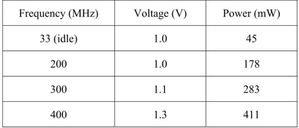
Table 1 and Table 2 show the valid CPU frequency, corresponding voltage and power consumption in Intel PXA255 and PXA270 CPUs, respectively. The power consumption values are different from the theoretical values calculated from equation (1), because most of DVS researches did not consider the short circuit and leakage power consumptions [1]. So it is more reasonable to adopt realistic power consumption values instead of those from equation (1) in DVS algorithms. In this

thesis, we used the power consumption values directly from Table 1 and Table 2 for evaluation.

Table 1：Power consumption specification for Intel PXA255.

Frequency (MHz) Voltage (V) Power (mW)

33 (idle) 1.0 45

200 1.0 178

300 1.1 283

400 1.3 411

Table 2：Power consumption specification for Intel PXA270.

Frequency (MHz) Voltage (V) Power (mW)

13 (idle) 0.85 44.2 104 0.9 115 208 1.15 279 312 1.25 390 416 1.35 570 520 1.45 747 624 1.55 925

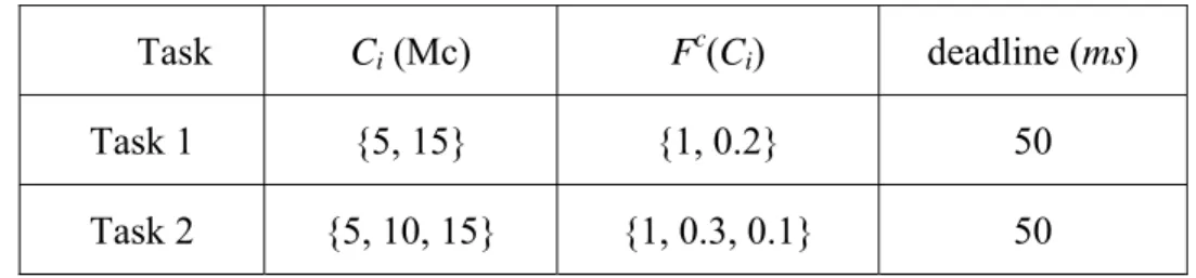
For illustration, we use PACE and our proposed OSRC, respectively, to find optimal schedules in realistic CPUs for two example tasks. Table 3 gives the specifications of these two tasks.

14

Table 3：Specifications of two example tasks

Task Ci (Mc) Fc(Ci) deadline (ms)

Task 1 {5, 15} {1, 0.2} 50

Task 2 {5, 10, 15} {1, 0.3, 0.1} 50

4.2 PACE Approach: Rounding the Frequencies

Obtain from PACE to the Nearest Available

Frequencies

First, we take task 1 running at Intel PAX255 as an example. From equation (8), if the start-up speed of task 1 is c and task 1 takes 5 million cycles (Mc) and keeps running, the CPU speed should be raised to 1.71c. By equation (8), we found the start-up speed c is 217 MHz, and the speed after 10 Mc is 370 MHz. Because Intel PXA255 does not support these speed settings, it is reasonable to choose the upper nearest available frequencies to avoid deadline missing. After rounding the ideal frequencies, the speed schedule is: 300 MHz at start-up and 400 MHz after 5 Mc executed. We use function p(f) which is C_eff ⋅ f 3to describe the power consumption

under speed f and p(f) can be obtained from Table 1. Now we rewrite equation (5) as

∑

From equation (9), the expected energy consumption is 7.15 mJ if the energy consumption during idea time is included.

Now we take task 2 running at Intel PXA255 as another example. By a similar way, based on PACE, we obtained an optimal schedule of {213 MHz, 319 MHz, 460 MHz}. Because the maximum supported frequency in Intel PXA255 is 400 MHz, we

could not find a rounding up frequency for 460 MHz.

4.3 OSRC Approach

Denoting the available frequencies by a linear combination was often used [22][25][26][27][28]. By rewriting the objective function (5), the stochastic DVS model is formulated to MKP. If a CPU has a limited set of m speeds, {s1, s2,…,sm}, it is better to formulate the original constrained nonlinear programming problem (equations (9) and (6)) as MKP. We denote f_i, the CPU frequency after a task

executes Ci-1 cycles and is static until the task executes Ci cycles, as a linear combination ofs_i m i m i i i s x s x s x f = ₁⋅ _,1+ ₂⋅ _,2+...+ ⋅ _, (10) where 1 , 1 =

∑

Using the same concept of the linear combination of frequencies, the expected energy consumption (E(fi)) by executing (Ci−Ci−1) cycles under static CPU frequency

} ,..., {1 m i s s f ∈ , can be rewritten as m i m i i i e s x e s x e s x f E( )= ( 1)⋅ ,1+ ( 2)⋅ ,2+...+ ( )⋅ , where i i i i i s C C s p s e( )= ( )⋅( − −1)

From equation (5), the expected energy consumption based on the intra task DVS stochastic model is the sum of the expected energy consumption in partition[Ci−1,Ci).

Therefore, the expected energy consumption under a limited set of frequencies combinations is

16 j i n i m j j i c n i i i c _{C E f F C e s x} F , 1 1 1 1 1) ( ) ( ) ( ) ( ⋅ =

∑∑

∑

From equation (6), we denote the time consumption of CPU executing (Ci−Ci−1)

cycles under speed si as ti(sj), which equals to (Ci−Ci−1)/sj. Thus, the total time

consumption by a task is the sum of ti(sj), and the time constraint under a limited set

of frequencies combinations is given by

d x s t n i m j j i j i ⋅ ≤

∑∑

Note that the equal (“=”) relation in equation (6) is replaced by less than and equal to (“≦”) relation. This is because under a limited set of frequencies, the sum of

j i j

i s x

t ( )⋅ _, is hard to fit the deadline exactly. Now the problem is MKP. x_i,_jare the

only variables that we should solve

Minimizing n _ij i m j j i c x s e C F , 1 1 1) ( ) ( ⋅ ⋅

∑∑

∑∑

∑

In an intra-task DVS schedule, the maximum number of frequency changes during a task running is the number of CPU frequency levels minus one. Because the frequency levels of realistic CPUs [15][16][17][18] are only a few, we use the

Dynamic Programming method to solve MKP [31]. From section 3.2, a task consists

of n partition, {p1, p2, ..., pn}={C1,C2−C1,...,Cn−Cn−1}, and the best feasible solution

of r partitions {pi … pn}, wherer=n−i+1, is denoted as Sr, which is a set of {xi,j …

⎪ ⎪ ⎩ ⎪ ⎪ ⎨ ⎧ ⋅ + > ∪ − ≥ = = − − + − − − minimal. is ) ( ) ( ) ( and 1, r } { , speed minimal the is and 1, r } { miss, deadline if null 1 , 1 1 1 1 , j r n c r j j r n r n n j j n r s e C F S E x S d C C s x S

Note that the deadline of Sr is given by

⎩ ⎨ ⎧ − = = − + ( ) otherwise. , if 1 n r j r r s t d n r d d

Because the deadline of Sr-1 varies with a selected speed sj in partition pn-r+1, the energy consumption of Sr-1 is given by

∑

And the time consumption by Sr-1 is given by

}. , ... {1, ) ( ) ( 2 1 t s j m S T n r n i j i r =

∑

In Sr , under the following two conditions, deadline miss will occur: 1) Sr-1 is null

2) Sr-1 is not null, but for all j∈{1,... ,m}, such that

r j r n r t s d S T( ₋₁)+ _{− +1}( )> Procedure Discrete-Optimal-Speed(Sr)

if (r == 1) then /*S1means the last partition.*/

Find minimum speed sj≧ (Cn-Cn-1)/d1; if (found sj) then

return {xn,j};

else

return null; else

for ( (every sj) and (T(Sr-1) + tn-r+1(sj) ≦dr) ) do

temp_S[j] = Discrete-Optimal-Speed(Sr-1);

end for

for (each temp_S[j]) do

Find j where Ej(Sr-1) + Fc(Cn-r)*e(sj) is minimum;

best_j = j;

end for

if (found best_j) then

return {xn-r+1, best_j}∪temp_S[best_j];

else

return null; end if

end if

18

The proposed OSRC procedure is shown in Fig. 1. Although a recursive procedure is used in the OSRC procedure, the computation will not take too much time due to a limited set of available CPU frequencies. Because voltage scaling is computationally expensive and hampers the possible energy saving [32], the size of n (number of a task’s possible execution cycles) should be small. In addition, the main idea of stochastic DVS is if a periodic task’s actual execution cycles (AEC) follows a distribution, the optimal speed schedule can save the most energy. Since the distribution can be obtained offline or online, the optimal speed schedule needs to be calculated only once and will be used for a long time. Based on the above, the computation time of stochastic intra-task DVS will not be an issue.

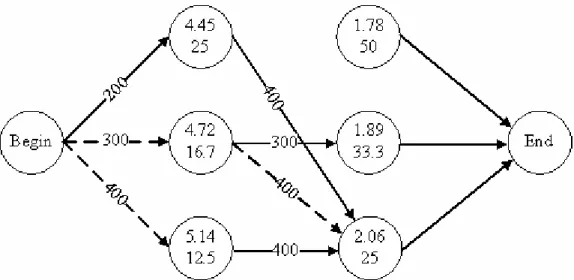
To demonstrate the merit of our OSRC over PACE, let’s return to example task 1, as shown in Table 3, which consists of two partitions{p₁, p₂}={C₁,C₂ −C₁}=

Mc} 10 Mc, 5

{ , and the corresponding tail distribution functions are 1 and 0.2. Fig. 2 shows a recursion graph for task 1. Note that each line is labeled with a selected frequency, the dotted lines present possible paths and the solid lines present the optimal paths. Each node is labeled with two values: the upper value is energy consumption and the lower value is time consumed in each partition. Our goal is to find a path which has a minimum sum of energy consumption, and the sum of time consumed must be less or equal to the deadline. Therefore, by using OSRC, the optimal speed schedule is {200 MHz, 400 MHz}, and the energy consumption is 6.51

mJ, which reduce 18% more power than that by using PACE (7.15 mJ from section

4.2). Similarly, by using OSRC, the optimal speed schedule of example task 2 is {200 MHz, 400 MHz, 400 MHz}, which couldn’t be solved by PACE, as shown in section 4.2.

20

Chapter 5

Evaluation and Discussion

5.1 Simulation Model

First, we examined our optimal speed procedure in CPUs with different frequency/voltage levels: Intel PXA255 and PXA270. The energy consumption with respect to each frequency/voltage was according to Table 1 and Table 2, and the energy consumption in idle state was also considered. A single task’s WCEC was set to the worst case execution time(WCET)×f_max; the WCET equals to 50 ms and

max

f means the maximum CPU frequency. α∈{0.2,0.5,0.8}, which is the ratio of

best case execution cycles (BCEC)/WCEC, means the variation of a task’s AEC

which is between BCEC and WCEC according to normal distribution [5][32]. The mean and standard deviation were set to (WCEC+BCEC) 2 and (WCEC−BCEC) 6, meaning that 99.7 percent of the execution cycles falls in the interval [BCEC, WCEC] [13]. Because the speed schedule varies with the CPU utilization, we simulated the task’s allowed execution time (AET) between[WCEC fmax,WCEC fmin]. All simulation

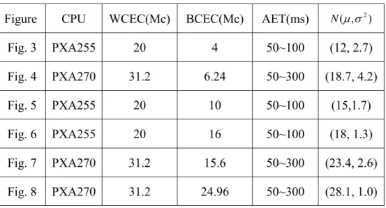
Table 4：Simulation parameters

Figure CPU WCEC(Mc) BCEC(Mc) AET(ms) (_µ,_σ2)

N Fig. 3 PXA255 20 4 50~100 (12, 2.7) Fig. 4 PXA270 31.2 6.24 50~300 (18.7, 4.2) Fig. 5 PXA255 20 10 50~100 (15,1.7) Fig. 6 PXA255 20 16 50~100 (18, 1.3) Fig. 7 PXA270 31.2 15.6 50~300 (23.4, 2.6) Fig. 8 PXA270 31.2 24.96 50~300 (28.1, 1.0)

We have implemented four schemes, including OSRC for performance evaluation: ․ WCE-stretch [5]: The speed schedule assumes that the task will exhibit its

worst case behavior, and choose the minimum static frequency.

․ PACE [2] : The optimal speed schedule is calculated by the theoretical value in ideal CPU as described in section 4, and the unavailable frequencies are rounding up to the nearest available ones.

․ OSRC : The speed schedule is calculated by the proposed OSRC schedule in Fig. 1.

․ LB (low bound) : An oracle algorithm knows the AEC in advance.

Because of a limited set of CPU frequency/voltage levels, the unavailable frequencies were replaced by linear combinations of their two immediate frequencies in low bound schemes for maximum energy saving. Unlike other stochastic-related papers [2][5], the performance comparison is based on the expected energy consumption. And all schemes are normalized with respect to the WCE-stretch.

5.2 Impact of CPU Levels

22

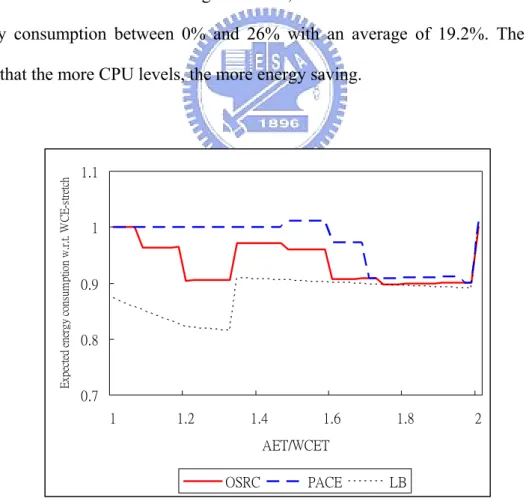
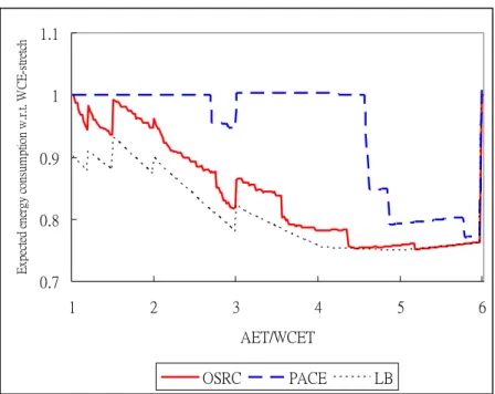
schemes in CPUs with different voltage/frequency levels: Intel PXA255 and PXA270. α is set to 0.2. In Fig. 3, the sudden transition between AET/WCET 1.2 and 1.4 in the low bound curve results in the WCE-stretch speed schedule drops the speed from 400 MHz to 300 MHz. When AET/WCET ≧ 2, the curve will up to 1 by the same reason. In 3 levels CPU, Intel PXA255, OSRC reduces CPU energy consumption between 0% and 10.2% with an average of 6.5%; PACE reduces CPU energy consumption between -1.2% and 9.9% with an average of 2.0%; the low bound scheme reduces CPU energy consumption between 0% and 18.5% with an average of 10.8%. In 6 levels CPU, Intel PXA270, OSRC reduces CPU energy consumption between 0% and 24.8% with an average of 15.9%; PACE reduces CPU energy consumption between -1.6% and 22.9% with an average of 5.6%; the low bound scheme reduces CPU energy consumption between 0% and 26% with an average of 19.2%. The results show that the more CPU levels, the more energy saving.

0.7 0.8 0.9 1 1.1 1 1.2 1.4 1.6 1.8 2 AET/WCET E xpe ct ed ene rgy cons um pt ion w .r.t . W CE -s tr et ch OSRC PACE LB

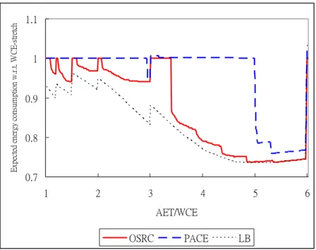
0.7 0.8 0.9 1 1.1 1 2 3 4 5 6 AET/WCET E xpe ct ed ene rgy cons um pt ion w .r.t . W CE -s tr et ch OSRC PACE LB

Fig. 4. The impact of CPU levels on expected energy consumption in Intel PXA270.

5.3 Impact of BCEC/WCEC(α) Ratio

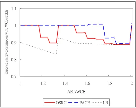
We set α to 0.5 and 0.8, and repeated simulations for these two types of CPUs. In Intel PXA255, as show in Fig. 5 and Fig. 6, OSRC can reduce 5.7% and 2.9% energy consumption in average (upper bound: 11.5% and 8.9%), respectively; the values in PACE are 2.1% and 1.0%. In Intel PXA270, as shown in Fig. 7 and Fig. 8, OSRC can reduce 13.4% and 6.7% energy consumption in average (upper bound: 17.3% and 13.3%), respectively; the values in PACE are 4.4% and 2.0%. These results show that when we set α to 0.5, the impacts of energy reduction are small for both types of CPU. But when we raised α to 0.8, the optimal schedules are close to the WCE-stretch scheme, especially in 3 levels CPU. Because low slack time limits the aggressive frequency/voltage reduction in the optimal schedule, it happens in all offline DVS schedules.

24 0.7 0.8 0.9 1 1.1 1 1.2 1.4 1.6 1.8 2 AET/WCE E xpe ct ed ene rgy cons um pt ion w .r.t . W CE -s tr et ch OSRC PACE LB

Fig. 5. The impact of

α

α

0.7 0.8 0.9 1 1.1 1 1.2 1.4 1.6 1.8 2 AET/WCET E xpe ct ed ene rgy cons um pt ion w .r.t . W CE -s tr et ch OSRC PACE LB

0.7 0.8 0.9 1 1.1 1 2 3 4 5 6 AET/WCE E xpe ct ed ene rgy cons um pt ion w .r.t . W CE -s tr et ch OSRC PACE LB

Fig. 7. The impact of

α

α

0.7 0.8 0.9 1 1.1 1 2 3 4 5 6 AET/WCE E xpe ct ed ene rgy cons um pt ion w .r.t . W CE -s tr et ch OSRC PACE LB

Fig. 8. The impact of

α

α

26

OSRC is three times in average better than that of PACE for realistic CPUs.

Table 5：Average energy saving percentage with respect to WCE-stretch Figure OSRC PACE LB

Fig. 3 6.5% 2.0% 10.8% Fig. 4 15.9% 5.6% 19.2% Fig. 5 5.7% 2.1% 11.5% Fig. 6 2.9% 1.0% 8.9% Fig. 7 13.4% 4.4% 17.3% Fig. 8 6.7% 2.0% 13.3%

Chapter 6

Conclusions and Future Work

6.1 Concluding Remarks

In this thesis, we have derived an optimal speed schedule for ideal CPUs for hard real-time systems by the Lagrange multiplier procedure, in a simple and elegant way, compared to PACE [2]. Because of limited available frequency/voltage levels in realistic CPUs, the optimal speed schedule for ideal CPUs can not be applied to realistic CPUs directly. To find an optimal speed schedule for realistic CPUs, we transform the original nonlinear programming problem into MKP based on the frequency/voltage levels and power consumption of a realistic CPU. With limited CPU frequency/voltage levels, the problem can be solved by the OSRC procedure feasibly. To evaluate the merits of the proposed OSRC, the actual data of Intel PXA255 and PXA270 CPU were used in the analysis. We have the following remarks. First, the analysis results have shown that the poor energy saving by using PACE in realistic CPUs, which is almost the same as that in WCE-stretch. By using the OSRC for realistic CPUs, the results are very close to the low bound derived from an oracle algorithm. Secondly, we observed that the CPU frequency/voltage levels affect the energy efficiency of the optimal speed schedule in the stochastic DVS model: the more the levels, the more the energy saving. Thirdly, we found that compiler-assisted intra-task DVS algorithms are hard to collaborate with inter-task DVS algorithms if the frequency/voltage scaling code is inserted in the source code. Lastly, under the

28

stochastic DVS model, our scheme can provide the best solution for realistic CPUs using dynamic programming. Evaluation have shown that the energy saving of OSRC is three times in average better than that of PACE in Realistic CPUs.

6.2 Future Work

In stochastic DVS intra-task DVS algorithms, the speed schedule is only calculated once for different AET so that it is easy to work with most of inter-task DVS algorithms. But there still exists some unresolved issues in OSRC. First, all of the approaches addressed in this thesis neglect the time and energy consumption owing to frequency/voltage transitions. If the time of transitions takes too long, a task may miss the deadline. If the energy consumption due to transitions is too much, it reduces the energy saving efficiency. It may even wastes more energy than a non-DVS speed schedule in the worst case. Secondly, if a task has been preempted and then rescheduled, the pre-calculated optimal speed schedule may fail because the AET of the task may become different. These problems deserve for further investigation.

Bibliography

[1] B. Moyer, “Low-Power Design for Embedded Processors,” in Proc. of the IEEE, vol. 89, no. 11, November 2001, pp. 1576-1587.

[2] J.R. Lorch and A.J. Smith, ”PACE: A New Approach to Dynamic Voltage Scaling,” IEEE Trans. on Computers, vol. 53, no. 7, pp. 856-869, July 2004.

[3] C. M. Krishna and Y. H. Lee, “Voltage-Clock-Scaling Adaptive Scheduling Techniques for Low Power in Hard Real-Time Systems,” IEEE Trans. on

Computers, vol. 52, no. 12, pp. 1586-1593, December 2003.

[4] D. Zhu, D. Mosse, and R. Melhem, “Power-Aware Scheduling for AND/OR Graph in Real-Time Systems,” IEEE Trans. on Parallel and Distributed Systems, vol. 15, no. 9, pp. 849-864, September 2004.

[5] F. Gruian, “Hard Real-Time Scheduling for Low-Energy Using Stochastic Data and DVS Processors,” in Proc. of ISLPED, 2001, pp. 46-51.

[6] N. AbouGhazaleh, D. Mosse, B. Childers, R. Melhem, and M. Craven, ”Collaborative operating system and compiler power management for real-time applications,” in Proc. of IEEE RTAS, 2003, pp. 133-141.

[7] Y. Zhu and F. Mueller, “Feedback EDF Scheduling Exploiting Dynamic Voltage Scaling,” in Proc. of IEEE RTAS, 2004, pp. 84-93.

[8] P. Pillai and K. G. Shin, “Real-Time Dynamic Voltage Scaling for Low-Power Embedded Operating Systems,” in Proc. of 18th ACM Symposium on Operating

30

[9] E. Chan, K. Govil, and H. Wasserman, “Comparing Algorithms for Dynamic Speed-Setting of a Low-Power CPU,” in Proc. of First ACM International

Conference on Mobile Computing and Networking, pp. 13-25, Nov. 1995.

[10] D. Shin, S. Lee, and J. Kim, “Intra-Task Voltage Scheduling for Low-Energy Hard Real-Time Applications,” IEEE Design and Test of Computers, Mar. 2001, pp. 20-30.

[11] W. Kim, D. Shin, H. Yun, J. Kim, and S. Min, “Performance comparison of dynamic voltage scaling algorithms for hard real-time systems”, in Proc. of IEEE

RTAS, 2002, pp. 219-228.

[12] Laptop and Notebook Computers, Toshiba, http://www.toshibadirect.com/td/b2c /toshibanotebook.to

[13] H. Aydin, R. Melhem, D. Mosse and P.M. Alvarez, “Power-Aware Scheduling for Periodic Real-Time Tasks,” IEEE Trans. Computers, vol.53, no. 5, pp. 584-600, May 2004.

[14] J. Seo, T. Kim, and C. Chung, "Profile-based Optimal Intra-task Voltage Scheduling for Hard Real-Time Applications," in Proc. of the 41st annual

Conference on Design Automation, pp. 87-92, June 2004.

[15] Intel. PXA255 Processor Electrical, Mechanical, and Thermal Specification, 2004.

[16] Intel. PXA270 Processor Electrical, Mechanical, and Thermal Specification, 2004.

[17] Product Information, http://www.amd.com/us-en/Processors/ProductInformation /0,,30_118,00.html

[19] D. Shin and J. Kim, “A Profile-Based Energy-Efficient Intra-Task Voltage Scheduling Algorithm for Hard Real-Time Applications,” in Proc. of ISLPED, 2001, pp. 271-274.

[20] M. Weiser, B. Welch, A.Demers, and S. Shenker, “Scheduling for Reduced CPU Energy,” in Proc. of First Symposium on Operating Systems Design and

Implementation, pp. 13-23, Nov. 1994.

[21] T. Ishihara and H. Yasuura, “Voltage scheduling problem for dynamically variable voltage processor,” in Proc. of International Symposium on Low Power

Electronic and Design, 1998, pp. 197-202.

[22] Y. Yu and V. K. Prasanna, “Resource Allocation for Independent Real-Time Tasks in Heterogeneous Systems for Energy Minimization,” Journal of

Information Science and Engineering,” vol. 19, no. 3, May 2003, pp. 433-449.

[23] T.A. Feo and M.G.C. Resende, “Greedy Randomized Adaptive Search Procedures,” Journal of Global Optimization, 6, pp. 109-133, 1995.

[24] R. L. Rardin, “Optimization in Operations Research,” Prentice-Hall, 1998. [25] B. Mochocki, X. Hu, and G. Quan, “A Realistic Variable Voltage Scheduling

Model for Real-Time Applications,” in Proc. of the IEEE/ACM International

Conference on Computer-aided design, 2002, pp. 726-731.

[26] Y. Zhang, X Hu, and D. Chen, “Task Scheduling and Voltage Selection for Energy Minimization,” in Proc. of the 39th

Conference on Design automation,

2002, pp. 183-188.

[27] A. Andrei, M. Schmitz, P. Eles, Z. Peng, and B. Al-Hashimi,

“Overhead-Conscious Voltage Selection for Dynamic and Leakage Energy Reduction of Time-Constrained Systems,” in Proc. of the Conference on Design,

32

[28] W. Kwon and T. Kim, “Optimal Voltage Allocation Techniques for Dynamically Variable Voltage Processors,” in Proc. of IEEE DAC’03, 2003, pp. 125-130. [29] T.L. Matrin and D.P. Siewiorek,” The Impact of Battery Capacity and Memory

Bandwidth on CPU Speed-Setting: A Case Study,” in Proc. of ISLPED, Aug, 1999, pp. 200-205.

[30] F. Yao, A. Demers, and S. Shenker, “A Scheduling Model for Reduced CPU Energy,” in Proc. of IEEE FOCS, 1995, pp 374.

[31] R. C. T. Lee, R. C. Chang, S. S. Tseng, and Y. T. Tsai, “Introduction to the Design and Analysis of Algorithms," Unalis corporation, 1999.

[32] Y. Shin and K. Choi, “Power Conscious Fixed Priority Scheduling for Hard Real-Time Systems,” in Proc. of 36th

Design Automation Conf., pp. 134-139,

1999.

[33] A. Andrei, M. T. Schmitz, P. Eles, Zebo Peng and B. M. Al Hashimi,

“Quasi-Static Voltage Scaling for Energy Minimization with Time Constraints,” in

Proc. of Design Automation and Test in Europe Conf., pp. 514-519, March, 2005.

[34] G. Sudha Anil Kumar and G. Manimaran, “An Intra-task DVS Algorithm Exploiting Path Probabilities for Real-time Systems,” in SIGBED Review, vol. 2, no. 2, April 2005.

[35] R. Amstrong, D. Kung, P. Sinha and A. Zoltners, “A Computational Study of Multiple Choice Knapsack Algorithm,” ACM Trans. on Mathematical Software, vol. 9, no. 2, pp. 184-198, June 1983.