國立交通大學
電子工程學系 電子研究所碩士班
碩 士 論 文
抵抗能量攻擊法的雙域橢圓曲線密碼運算單元之設計
與實現
Design and Implementation of a Dual-Field Elliptic
Curve Cryptographic Processor with Power Analysis
Countermeasures
學生:陳耀琳
指導教授:李鎮宜 教授
抵抗能量攻擊法的雙域橢圓曲線密碼運算單元之設計
與實現
Design and Implementation of a Dual-Field Elliptic
Curve Cryptographic Processor with Power Analysis
Countermeasures
研 究 生:陳耀琳
Student:Yao-Lin Chen
指導教授:李鎮宜教授
Advisor:Chen-Yi Lee
國 立 交 通 大 學
電子工程學系 電子研究所 碩士班
碩 士 論 文
A ThesisSubmitted to Department of Electronics Engineering & Institute Electronics College of Electrical and Computer Engineering
National Chiao Tung University In Partial Fulfillment of the Requirements
for the Degree of Master of Science
in
Electronics Engineering July 2009
抵抗能量攻擊法的雙域橢圓曲線密碼運算單元
之設計與實現
學生:陳耀琳
指導教授
:李鎮宜
國立交通大學電子工程學系 電子研究所碩士班
摘
要
在這篇論文中,我們提出了一個可支援雙域有限域運算以及可支援任意
橢圓曲線運算的雙域橢圓曲線密碼運算單元。透過我們提出的通用演算法,
這個運算單元的執行週期數大幅的降低。藉由我們提出的面積共用方法以及
梯子選擇法,我們 160 位元以及 256 位元的雙域橢圓曲線密碼運算單元的面
積在聯電 90 奈米製程下只須 0.29mm
2和 0.45mm
2。此外,運算單元的操作面
積也可以透過我們提出的指數判定器以及資料路徑分離法可大幅的提升。我
們也提出一個可以對抗能量攻擊法的雙域橢圓曲線密碼運算單元。透過我們
提出的通用亂數演算法,我們面積的損失僅僅 8.4%。
Design and Implementation of a Dual-Field Elliptic Curve
Cryptographic Processor with Power Analysis Countermeasures
student:Yao-Lin Chen
Advisors:Chen-Yi Lee
Department of Electronics Engineering & Institute of Electronics
National Chiao Tung University
ABSTRACT
In this thesis, we propose a high-performance dual-field elliptic curve
cryptographic processor (DECP) architecture that can support all finite field
operations and elliptic curve (EC) functions with arbitrary field and curve. Based
on our proposed fast unified division algorithm, the operation cycles can be
significantly reduced. Compared with previous works using high radix
multiplication in projective coordinate, our 160-bit and 256-bit DECPs can
achieve competitive performance in terms of execution cycles with only 0.29mm
2and 0.45mm
2silicon area in UMC 90nm CMOS technology by exploiting
hardware sharing and ladder selection techniques. In addition, the operating
frequency in prime field and binary field can be increased due to the proposed
data-path separation and degree checker. To resist power analysis attack, we
propose a DECP with power analysis countermeasures architecture based on the
proposed unified random algorithms with only 8.4% area overhead.
誌
謝
研究生活,剎那間的消逝。兩年中,常和實驗室的大家一起研究到早晨、一起唱歌、 一起談心。在 Si2 和 STAR 遇到許多很棒的人,是我一輩子想珍藏的。嘴砲的義澤、很娘 聲音很高的明諭、老到掉渣又很寶的浩民、很照顧大家的均宸、貼心又窩心的建辰、一直 把咩的佳龍、給我很多方向以及建議的 STAR 領導人柏均、常常關心我的義閔、幫我改英 文的人偉、好夥伴勇志、很熱心的曜哥、很八卦的欣儒、人很好的如宏、嘴巴很機車但心 地不錯的靜瑜、投球很猛的廷聿、幫我改機的歐陽、說話不算話的昱帆、我的女朋友憲平、 嘴巴功力真是一流的智翔、給我很多幫助的小馬、很黑但人很 nice 的書餘、又壯又很厲 害的偉豪、衝浪少年芳年、大發慈悲給我研究費的好媽媽子菁和伶霞、看起來很靦腆的易 蓁、比我小就當助理的桂綸鎂立瑜、問不到我名字又被我叫純美的婷美、講話很斯文的美 玲。遇到他們真的是我一輩子的福氣,真的很謝謝他們。一路上,交大的老師們給我許多 的指導和照顧。指導老師李鎮宜老師每次在會議中,都會給我許多大方向的建議,讓我對 我的研究更加有目標、STAR 的指導老師張錫嘉老師,對我們都很照顧,關心我們的生活 以及研究、系上老師江蕙如老師,在研究方向上給我許多鼓勵,透過她的推薦,讓我在研 究所考試得到很棒的成績,老師人真的很好很好。 最後,我要感謝我的家人。謝謝他們一直以來的鼓勵,從幼稚園、小學、國中、高 中、大學、研究所,無怨無悔的照顧,真的很謝謝他們。在大學求學的這段時間,很謝謝 佩蓉的陪伴,在我快樂時候陪我分享喜悅,在我失意的時候陪我分享悲傷。也很謝謝一路 上陪我成長的朋友們,幼幼社的麻吉們以及交大電子系的大家。真的很謝謝你們,因為有 你們,才有今天的陳耀琳,謝謝你們,謝謝。
Contents
1 Introduction 1
1.1 Elliptic Curve Cryptography . . . 1
1.2 Power Analysis . . . 2
1.3 Organization . . . 3
2 Preliminary of Elliptic Curve Cryptography Cryptosystem 4 2.1 Point Addition and Doubling over Finite Fields . . . 5
2.2 Analysis of Point Addition and Doubling in Different Coordinates . . . 6
2.3 Elliptic Curve Point Scalar Multiplication Methods . . . 7
2.4 Galois Field Arithmetic . . . 8
2.4.1 Unified Multiplication Algorithms . . . 9
2.4.2 Unified Inversion and Division Algorithms . . . 11
2.5 Elliptic Curve Cryptographic Applications . . . 18
2.5.1 Elliptic Curve Data En/Decryption . . . 18
2.5.2 Elliptic Curve Based Protocols . . . 18
2.6 Power Analysis Attacks and Countermeasures . . . 19
2.6.1 Simple Power Analysis . . . 19
2.6.2 Differential Power Analysis . . . 20
3 Proposed Unified Algorithms 23 3.1 Unified Division Algorithm . . . 23
3.2 Unified Multiplication Algorithm . . . 30
3.3 Unified Random Algorithms . . . 31
3.3.1 Unified Random Division Algorithm . . . 31
4 Proposed Architectures 35
4.1 Galois Field Arithmetic Unit . . . 35
4.1.1 Data-path Separation . . . 36
4.1.2 Hardware Sharing . . . 37
4.1.3 Degree Checker . . . 39
4.1.4 Ladder Selection . . . 39
4.2 Dual-Field Elliptic Curve Cryptography Processor . . . 40
4.3 Dual-Field Elliptic Curve Cryptography Processor with Power Analysis Countermeasures . . . 42
5 Implementation Results 47 5.1 Galois Field Arithmetic Unit . . . 47
5.2 Dual-Field Elliptic Curve Cryptography Processor . . . 48
5.3 Dual-Field Elliptic Curve Cryptography Processor with Power Analysis Countermeasures . . . 50
6 Conclusion and Discussion 57 A Appendix 58 A.1 Duality of Multiplication and Division . . . 58
A.2 Power Analysis Attack on The Dual-Field Elliptic Curve Cryptographic Processors . . . 58
A.3 Unified Division Algorithm Based on Takagi’s Algorithm . . . 59
A.4 Word-based Unified Multiplication/Division Architecture . . . 61
List of Figures
2.1 Hierarchical organization of EC protocol . . . 4
2.2 The component of ECSM operation . . . 5
2.3 (a) A ECADD power trace. (b) A ECDBL power trace. (c) A ECSM power trace. . . 20
2.4 Simple DPA attack flow . . . 22
2.5 Correlation coefficients of key value,[ki = 0, ki−1 = 0, ki−1 = 1, ki−1 = 0], for (a) unprotected chip (b) protected chip. . . 22
4.1 Architecture of R2-GFAU. . . 36
4.2 Architecture of R4-GFAU. . . 37
4.3 Data-path separation method. . . 38
4.4 (a) The degree checking architecture by intuitive implementation. (b) Ar-chitecture of degree checker. . . 40
4.5 The data post-operation by intuitive implementation. . . 40
4.6 Architecture of ladder selection. . . 41
4.7 Architecture of DECP. . . 44
4.8 The flow chart of DECP. . . 45
4.9 Architecture of R2-DECPAC. . . 45
4.10 Flow Chart of R2-DECPAC. . . 46
5.1 (a) Layout of 160-bit R4-DECP chip. (b) Layout of 256-bit R4-DECP chip. 50 5.2 Random test on a 32-bit pseudo number generator. . . 51
A.1 The environment of PA attacks. . . 59
A.2 The GF(p) architecture of proposed w-UM/D. . . 62
A.4 The architecture of MM operation over GF(2m). . . 64 A.5 The architecture of the proposed ECC processor. . . 65
List of Tables
1 Mathematical symbols . . . vii
2 Abbreviations . . . viii
2.1 ECDBL and ECADD. . . 6
2.2 ECDBL and ECADD for various coordinates over GF(p). . . 7
2.3 ECDBL and ECADD for various coordinates over GF(2m). . . . 7
2.4 Galois field arithmetic. . . 8
2.5 The properties of Kaliski’s unified inversion algorithm. . . 15
2.6 The properties of Takagi’s unified modular division algorithm. . . 16
3.1 The properties of R2-UD. . . 23
3.2 The invariant equivalences of the proposed R2-UD algorithm for MMD operation. . . 24
3.3 The invariant equivalences of the proposed R2-UD algorithm for MD op-eration. . . 25
3.4 The example of the proposed R2-UD. . . 25
3.5 The properties of the proposed R4-UD. . . 26
3.6 Operating steps of MMD/MD operations over dual fields of previous works. 34 3.7 Performance Analysis of Division Operation. . . 34
4.1 Details of hardware sharing method in R2-GFAU. . . 38
4.2 Details of hardware sharing method in R4-GFAU. . . 39
4.3 Performance Analysis of R2-DECP. . . 42
4.4 Performance Analysis of R4-DECP. . . 43
4.5 Performance Analysis of R2-DECPAC. . . 44
5.1 Comparisons among 256-bit finite field designs over GF(p). . . 48
5.2 Implementation results of proposed 256-bit GFAU over GF(2m). . . 49
5.3 Implementation results of 256-bit R2/4-DECP over GF(p). . . 50
5.4 Implementation results of 256-bit R2/4-DECP over GF(2m). . . 51
5.5 Comparisons among 521-bit ECC designs over GF(p). . . 52
5.6 Comparisons among 521-bit ECC designs over GF(2m). . . 52
5.7 Comparisons among 160-bit ECC designs over GF(p). . . 52
5.8 Comparisons with 160-bit ECC designs over GF(2m). . . 53
5.9 Comparisons among 256-bit ECC designs over GF(p). . . 53
5.10 Comparisons among 256-bit ECC designs over GF(2m). . . 54
5.11 Comparisons among 571-bit ECC designs over GF(2m). . . 54
5.12 Implementation results of 256-bit R2-GFAUPAR. . . 55
5.13 Implementation results of 256-bit R2-DECPAR. . . 55
5.14 Comparisons among 521-bit ECC designs over GF(p). . . 55
5.15 Comparisons among 521-bit ECC designs over GF(2m). . . 56
A.1 Duality of division and multiplication. . . 58
A.2 The detail environment of PA attacks. . . 59
A.3 Implementation results of 256-bit GF(p) division algorithms. . . 61
A.4 Implementation results of ECC processors over GF(2m). . . 64
List of Notations
Table 1: Mathematical symbols
Definition Description Definition Description E() Elliptic curve L, K Fields P, Q, G Points in EC O A point at infinity
p Prime m Field size
n Maximum field size i, j, l Variables
k Key A Affine
J Jacobian JM Modified Jacobian
JC Chudnovsky Jacobian LP Lopez projective
LM
LP with Montgomery
LM C
LM with common Z
ladder algorithm projective coordinate X, Y Integer U, V, R, S, T, D Operands
r Random number H() Hash function x x-coordinate y y-coordinate
of a point of a point
M Message N Curve order
Table 2: Abbreviations
Definition Description Definition Description DECP Dual-field ECC processor EC Elliptic curve ECSM EC scalar point multiplication MD Modular division
MMD Montgomery MD MI Modular inversion MMI Montgomery MI MM Modular multiplication MMM Montgomery MM MA Modular addition
MS Modular subtraction PA Power analysis ECDBL EC point doubling ECADD EC point addition ECSUB EC point subtraction D Division
M Multiplication SQ Squaring
A Addition S Subtraction
UD Unified division R2-UD Radix-2 UD R4-UD Radix-4 UD UM Unified multiplication R2-UM Radix-2 UM R4-UM Radix-4 UM
GFAU Galois field arithmetic unit R2-GFAU Radix-2 GFAU R4-GFAU Radix-4 GFAU R2-DECP Radix-2 DECP R4-DECP Radix-4 DECP PAC PA countermeasures R2-GFAUPAC R2-GFAU with PAC R2-DECPAC R2-DECP with PAC
FLT-UMI Unified MI FLT-UMMI Unified MMI based on FLT based on FLT K-UI Kaliski’s unified T-UMD Takagi’s unified
inversion MD
L-UD Liu’s UD MSQ Modular SQ
FT-UD UD based on T-UMD w-UM/D Word-based multiplication /division architecture AT Gates × time
Chapter 1
Introduction
1.1
Elliptic Curve Cryptography
To ensure the data security of network communication, public-key encryption algo-rithms have been widely adopted. Elliptic curve cryptography (ECC) [1–6] can provide the same security level as the Rivest, Shamir and Adleman (RSA) [7] algorithm with much reduced key-size. In ECC scheme, the major operation is the elliptic curve point scalar multiplication (ECSM). To reduce the execution time in software implementation [8], several accelerating hardware processors are proposed. Many ECC designs have been published over specified finite field, either GF(p) [9–11] or GF(2m) [12–22]. The designs over GF(2m) usually target at area constrainted applications such as smart cards or RFID cards due to the carry-free propagation and fixed irreducible polynomial in specific ECs. However, to support higher security level, both arbitrary key-size and field operations are essentially required. Some dual-field ECC processors (DECP), in which the coordinate is transformed to the projective coordinate to avoid inversion operations in ECSM, have been proposed up to now [23–25]. Satoh and Takano [23] exploit a r × r-bit multipliers to speed up the ECSM in the Jacobian’s projective coordinate, and Lai and Huang [24, 25] present a parallel architecture based on [23] to enhance the throughput. However, opera-tions in the projective coordinate are more complicated than that in the affine coordinate, and the inversion is still needed in coordinate transformation before and after the ECSM in projective coordinate. To reduce the execution cycles of ECSM and coordinate trans-formation, the size r of multipliers or the number of parallel units are increased, which
usually results in high hardware cost.
The traditional approach of inversion operation is based on the Fermat’s little theo-rem (FLT) [26]. It can be realized by repeating squaring and multiplication operation but results in longer execution time [23–25]. In 1995, Kaliski [27] proposed a unified inversion algorithm to accomplish the inversion operations. Several later algorithms and architec-tures are based on this algorithm [28–34]. Furthermore, to directly reduce the execution cycles of ECSM in affine coordinate, many architectures and algorithms [35–37] are based on Takagi’s modular division (MD) algorithm [38].
To solve the overhead of inversion and the following multiplication operation in ECSM and coordinate transformation, we propose a fast unified division algorithm supporting Montgomery modular division (MMD) and MD operations over dual fields. Note that the “unified” means the algorithm is able to handle dual-field operations. In addition, we apply hardware sharing method, data-path separation, and degree checker into a DECP to reduce the hardware cost and increase the operating frequency. Our DECP supports ECSM and finite field operations with arbitrary curves and parameters over dual fields. The implementation result shows our DECP outperforms relative works in functionality, hardware efficiency, execution time, and power consumption.
1.2
Power Analysis
Physical attacks on cryptographic devices using side-channel information are attract-ing extensive attention [39–41]. In order to reveal secret parameters, the power dissipation, electromagnetic radiation, or operating times (i.e. timing attack [42]) as correlated to in-ternal operation are measured. Simple power analysis (SPA) [43] and differential power analysis (DPA) [44, 45] are known as basic and powerful side-channel attacks, which have been discussed in several literatures [4, 46–51].
To resist the power analysis attack, we use the masking techniques to randomize the operating data. We propose a unified random division and a unified random multiplication algorithm to make the total random numbers equal 2m, where m is the field length. Compared with the proposed unified algorithms, the implementation of the unified random algorithms increases little hardware cost to resist DPA attack. In addition, the SPA attack
is resisted by well known double-and-add/sub-always method.
1.3
Organization
In this thesis, we propose the unified algorithms and ECC architectures to support the operations in elliptic curve cryptography, and propose the unified random algorithms and architectures to resist power analysis in cryptographic processor. In Chapter 2, the preliminaries of ECC cryptosystem is introduced. In Chapter 3, we propose the unified algorithms to accomplish the division and multiplication operations. In Chapter 4, we propose the Galois field arithmetic units and dual-field ECC processors to support finite field operations, EC functions, or power analysis countermeasures. In Chapter 5, we show the implementation results of our proposed architectures. In the last Chapter, we give a brief conclusion and discussion.
Chapter 2
Preliminary of Elliptic Curve
Cryptography Cryptosystem
Elliptic curve cryptography cryptosystem, which is based on the arithmetic on elliptic curves (ECs) over finite field, has been widely adopted in recent years. The arithmetic on ECs is the EC point scalar multiplication (ECSM) which is computed in Galois field. In addition, the applications of ECC are the EC data en/decryption and EC based protocols which are composed of ECSM, random number generator, hash function, and Galois field arithmetic. The relationship is given in a hierarchical organization as shown in Figure 2.1.
EC Data En/Decryption, ECDH, ECDSA, ECIES, ECMQV
ECC applications
Galois Field Arithmetics
Elliptic Curve Scalar Point Multiplication
EC functions
Modular Operations
Hash Function, Random Number Generator
Cryptographic functions
Figure 2.1: Hierarchical organization of EC protocol
The ECSM operation consists of four parts, which are operating field, coordinate, point multiplication method, and Galois field arithmetic, shown in Table 2.2. Furthermore, power analysis on ECC is discussed nowadays. By measuring power traces of ECC devices, the secret informations can be extracted. We will introduce some power analysis methods
and countermeasures to attack or resist them, respectively.
Field
Coordinate
Point Scalar Multiplication Method
Galois Field Arithmetic
Prime, Extension Binary
Affine, Projective, Jabobian s Projective...
Binary Method, Binary NAF Method, Montgomery Ladder... Modular Addition/ Subtraction,
Montgomery/Modular Multiplication/Division
Figure 2.2: The component of ECSM operation
2.1
Point Addition and Doubling over Finite Fields
If L and K are two fields, L ⊇ K, the general elliptic curve E defined over K is an equation of the form (also called Weierstrass equation)
E(L) : y2+ a1xy + a3y = x3+ a2x2+ a4x + a6, (2.1)
where a1,..., a6 ∈ K are constants and (x, y) ∈ L × L is the set of points along with a point O at infinity. The point O at infinity is defined as the identity element, i.e., P + O = O + P = P for all P ∈ E(L). Note that if P = (x, y), then the negation of P , denoted by −P , is defined as (x, −a1x − a3− y).
However, it is more practical to specify what kind of finite field of set x, y, a1, ..., and a6 belong to in equation 2.1. Most of ECC designs are implemented over GF(p) or GF(2m), where p is a prime integer and m is the field size determined by the key length. An equation form of the non-singular EC E(GF(p)) is given by
E(GF(p)) : y2 = x3+ ax + b (mod p), (2.2)
where a, b ∈GF(p) and 4a3+ 27b2 6= 0 (mod p). For two distinct points P = (x
1, y1) and Q = (x2, y2) with P 6= ±Q, the formulas of the EC point addition (ECADD) P + Q = (x3, y3) and EC point doubling (ECDBL) in affine coordinates are shown in Table 2.1. The ECDBL is that the point P adds itself, i.e., 2P = (x3, y3), but P 6= −P . For the existence of inverses, it is easy to return the value as O because P + (−P ) = O.
For GF(2m), the non-singular EC is an equation of this form
E(GF(2m)) : y2+ xy = x3+ ax2+ b (mod p), (2.3)
where a, b ∈GF(2m) and b 6= 0 (mod p) and p is an irreducible polynomial of degree m. Table 2.1 lists all the formulas of the point addition over GF(2m) and the point doubling in affine coordinates. Note that the EC point subtraction (ECSUB) Q−P with P = (x, y) can be computed by ECADD Q+(−P ), where the coordinates of −P are given by (x, −y) over GF(p) and (x, x + y) over GF(2m).
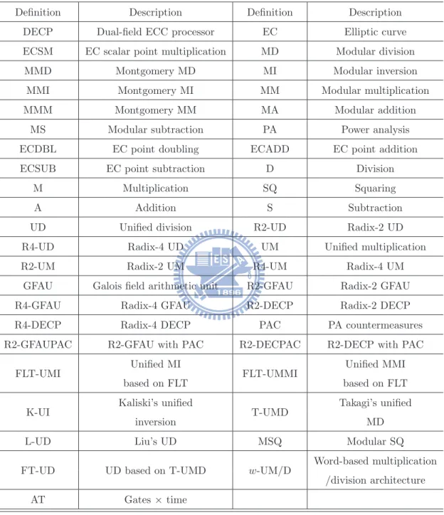
Table 2.1: ECDBL and ECADD.
Field Doubling(x3,y3)=2(x1,y1) Addition(x3,y3)=(x1,y1)+(x2,y2)
λ = 3x21+a 2y1 (mod p) λ = y2−y1 x2−x1 (mod p) GF(p) x3= λ2− 2x1 (mod p) x3= λ2− x1− x2 (mod p) y3= λ(x1− x3) − y1 (mod p) y3= λ(x1− x3) − y1 (mod p) λ = x1+yx1 1 (mod p) λ = y2+y1 x2+x1 (mod p) GF(2m) x 3= λ2+ λ + a (mod p) x3= λ2+ λ + x1+ x2+ a (mod p) y3= λ(x1+ x3) + x3+ y1 (mod p) y3= λ(x1+ x3) + x3+ y1 (mod p)
2.2
Analysis of Point Addition and Doubling in
Dif-ferent Coordinates
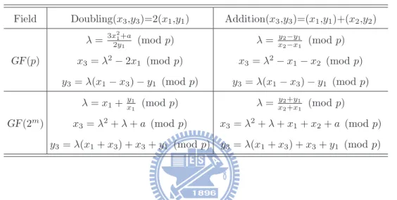
Traditionally, ECSM is operated in affine coordinate. To avoid the inversion operation which is more expensive than multiplication, many coordinates has been proposed, such as Jacobian projective coordinate [1] and L´opez projective coordinate [52], etc. Table 2.2 and 2.3 show the analysis of EC point doubling/addition in different coordinates [53]. The execution cycle of the ECSM in affine coordinate is dominated by the division operation. To outperform other coordinates, the execution cycle of division must be less than 5.2M c, where M c means the cycle of multiplication.
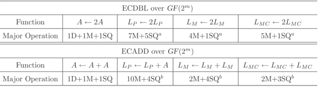
Table 2.2: ECDBL and ECADD for various coordinates over GF(p). ECDBL over GF(p) Function A ← 2A J ← 2J JM ← 2JM JC← 2JC Major Operation 1D+1M+2SQ 4M+6SQ 4M+4SQ 5M+6SQ ECADD over GF(p) Function A ← A + A J ← J + A JM ← JM + A JC← JC+ A Major Operation 1D+1M+1SQ 12M+4SQ 13M+6SQ 11M+3SQ
Table 2.3: ECDBL and ECADD for various coordinates over GF(2m).
ECDBL over GF(2m) Function A ← 2A LP ← 2LP LM ← 2LM LM C ← 2LM C Major Operation 1D+1M+1SQ 7M+5SQa 4M+1SQa 5M+1SQa ECADD over GF(2m) Function A ← A + A LP ← LP + A LM ← LM + LM LM C← LM C+ LM C Major Operation 1D+1M+1SQ 10M+4SQb 2M+4SQb 2M+3SQb a: Including the operation cycles of extra step.
2.3
Elliptic Curve Point Scalar Multiplication
Meth-ods
Intuitively, the ECSM operation, i.e. kP = P +P...+P , requires (k −1) iterative point addition to accomplish. To reduce the execution cycle, many methods such as binary method and window method were proposed [1]. Considering the hardware efficiency and operation cycles, we adopt the binary Non-adjacent form (NAF) method shown in algorithm 2.1. Prior to this algorithm, the secret key must be transformed to the NAF form. The details of the NAF is illustrated in [2].
Algorithm 2.1. (Binary NAF method for point multiplication.)
Input: P and k, where P ∈ E(L), k is an integer with NAF form and km−1 = 1. Output: Q = [k]P . 1. Q = P 2. for i = m − 2 to 1 by −1 do 3. Q = [2]Q 4. if ki = 1, then 5. Q = Q + P 6. else if ki = −1, then 7. Q = Q − P 8. end if 9. end for
2.4
Galois Field Arithmetic
Galois field arithmetic is very important not only in ECSM operations but also in EC protocols. Eight different modular operations over finite field are commonly used and details of these modular operations and their abbreviations are listed in Table 2.4. The division and multiplication are more complicated than addition and subtraction, so many approaches have been proposed to enhance the performance of division and multiplication.
Table 2.4: Galois field arithmetic.
Operations
Modular addition M A(X, Y ) = X + Y (mod p) Modular subtraction M S(X, Y ) = X − Y (mod p) Modular multiplication M M (X, Y ) = X · Y (mod p) Montgomery modular multiplication M M M (X, Y ) = X · Y · 2−m (mod p)
Modular inversion M I(X) = X−1 (mod p)
Montgomery modular inversion M M I(X) = X−1· 2−m (mod p)
Modular division M D(X, Y ) = X · Y−1 (mod p)
2.4.1
Unified Multiplication Algorithms
Unified Modular Multiplication AlgorithmThe unified MM computes R ≡ X · Y (mod p), where 0 ≤ X, Y < p or 0 ≤ deg(X), deg(Y ) < deg(p) over prime field or binary field, respectively. MM operation can be realized in two methods, left-to-right MM and right-to-left MM. The implementa-tion of these two methods are similar. Algorithm 2.2 shows the left-to-right unified MM (UMM) algorithm. Note that the addition/subtraction operations mean XOR gates in binary field, and the operation ”2·” represents ”x·” in binary field.
Algorithm 2.2. (Left-to-right unified modular multiplication.)
Input: X, Y , and p, where X, Y are n-bit integer over GF (p) or GF (2m) and p is the prime or irreducible polynomial.
Output: R ≡ X · Y (mod p). 1. R = 0, S = Y 2. for i from 0 to m − 1 by +1 do 3. R = (R + Xi· S) (mod p) 4. S = 2 · S (mod p) 5. endfor
High Radix Unified Montgomery Modular Multiplication Algorithm
The well known Montgomery multiplication algorithm, proposed by P. L. Montgomery [54], is commonly used to compute the modular multiplication without trial division. The concept of the MMM is to turn the MM into iterative operations with both addition and logic level shifting. Hence the MMM is quite appropriate for software or hardware implementation. The additional overhead is the pre-/post-processing stages of the domain transformation for the input/output. In the pre-processing stage, the data is transformed from integer domain, X · 20, to Montgomery domain, X · 2m. And in the post-processing stage, the data is transformed back to integer domain.
Algorithm 2.3 [54] computes R ≡ X · Y · 2−m (mod p), where 0 ≤ X, Y < p or 0 ≤ deg(X), deg(Y ) < deg(p) over prime field or binary field, respectively. Because the X and Y are in the Montgomery domain, the MMM computes X · Y · 2−m (mod p) to
make the output R still in the Montgomery domain. In order to use n · r-bit multiplier, an n-bit number needs to be divided into l r-bit blocks (i.e., n = l · r). The operand X can be represented by r-bit words Xi as X = Xl−1 · 2r(l−1)+ ... + X1· 2r+ X0. The Ti operation is used to make the least significant word of accumulated operand R be zero. The proof is shown as follows:
R + Xi· Y + Ti· p (mod 2r) = R + Xi· Y + (R0+ Xi· Y ) · q · p (mod 2r) = 0 (2.4) Therefore, the division operation is easily achieved by shifting r bit. Moreover, the operand R may excess p during the MMM iteration over prime field, so a reduction step after the last iteration is required. On the other hand, since deg(R) ≥ m would not occur in binary field operation, the recovery step is not required. Traditionally, the r is commonly set to 1 for low-cost design. The algorithm is shown in algorithm 2.4.
There is a variety of hardware architectures to implement the MMM. Both the systolic architecture [55] and the word-level architecture [56] exploit the pipelining techniques to shorten the critical path. Beside, Satoh and Takano proposed double loop method [23] to apply into MMM operation. Compared with architectures with n×r-bit multipliers, Satoh and Takano’s work just needs one r × r-bit multiplier to improve the MMM operation. Besides, the operation cycle increases from m+1 and m cycles to 2l2+4l+1 and 2l2+3l+1 over prime field and binary field [23], respectively.
Algorithm 2.3. (Radix-r unified Montgomery multiplication algorithm.) Input: X, Y , q, and p, where X, Y are n-bit integer over GF (p) or GF (2m) , q = −p−1 (mod 2r), and p is the prime or irreducible polynomial.
Output: R ≡ X · Y · 2−m (mod p). 1. R = 0 2. for i = 0 to l − 1 by +1 do 3. T = (R0+ Xi· Y ) · q (mod 2r) 4. R = Ri+Xi·Y +T ·p 2r 5. endfor
Algorithm 2.4. (Radix-2 unified Montgomery multiplication algorithm.) Input: X, Y , and p, where X, Y are in GF (p) or GF (2m) and p is the prime or irre-ducible polynomial. Output: R ≡ X · Y · 2−m (mod p). 1. R = 0 2. for i from 0 to m − 1 by +1 do 3. T = (R + Xi· Y ) 4. R = (T +T0·p) 2 5. endfor
6. if R ≥ p and the operating field is prime, then: R = R − p
2.4.2
Unified Inversion and Division Algorithms
Unified Inversion Algorithms based on Fermat’s Little Theorem
Based on Fermat’s Little Theorem (FLT), Xp−1 = 1 (mod p), the inversion opera-tion is easily achieved by X−1 = Xp−2 (mod p). FLT is commonly used in projective operation, because of low cost and high integration with radix-r MMM. Algorithm 2.5 shows the unified MMI algorithm based on FLT (FLT-UMMI), and the execution cycle of FLT-UMMI is about m2 ∼ 2m2, where m is the execution cycle of MMM. Besides, the FLT can also be used to accomplish MI operation shown in algorithm 2.6.
Algorithm 2.5. (Unified MMI algorithm based on FLT.)
Input: X · 2m and p, where X is in GF (p) or GF (2m) and p is the prime or irreducible polynomial.
Output: R ≡ X−1· 2m (mod p).
1. if the operating field is prime, then: T = p − 2 2. else: T = 2m− 2 3. R = X · 2m 4. for i from m − 2 to 0 by −1 do 5. R = M M M (R, R) 6. if Ti = 1, then: R = M M M (R, X · 2m) 7. endfor
Algorithm 2.6. (Unified MI algorithm based on FLT (FLT-UMI).)
Input: X and p, where X is in GF (p) or GF (2m) and p is the prime or irreducible polynomial.
Output: R ≡ X−1 (mod p).
1. if the operating field is prime, then: T = p − 2 2. else: T = 2m− 2 3. R = X 4. for i from m − 2 to 0 by −1 do 5. R = R · R (mod p) 6. if Ti = 1, then: R = R · X (mod p) 7. endfor
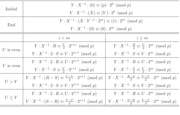
Kaliski’s Unified Inversion Algorithm
Algorithm 2.7 shows the unified inversion algorithm proposed by Kalisiki (K-UI) [27]. This algorithm supports the MI and MMI operation over dual fields. This algorithm calculates R = X−1 · 2m (mod p), where the operand R is defined as the Montgomery representation of modular inverse, m is the bit-length of p, and X (6= 0) be the elements of the field. Similarly, the R = X−1 (mod p) can also be obtained from this algorithm, where the operand R is defined as the integer representation of modular inverse. The inversion is computed by intertwining the procedure for finding the modular quotient with that for calculating gcd(X, p). The algorithm requires four operands, U , V , R, and S. U and V are used for calculating gcd(X, p) and the operands R and S are used for calculating modular inverse. The operands U and V are initialized to Y and p, respectively, and the properties shown in Table 2.5 are applied iteratively to calculate gcd(X, p). For example, U can be replaced by U/2 according to the property gcd(U, V ) = gcd(U/2, V ), when U is even. In addition, R and S are initialized to the values of X and 0, respectively. Besides, the corresponding R, S operations are determined by the following invariants:
( X · R ≡ −U · 2i (mod p)
X · S ≡ V · 2i (mod p) (2.5)
During the phase 1 operation which means the operating steps are 2∼8, the domain value i is increased by 1 every cycle. Table 2.5 shows the detail operations of U , V , R, and S
based on the properties and invariants. For instance, if U is even, the algorithm changes value U to U/2 and the value i is increased to i + 1 for obeying the equivalence 2.5. To increase the value i to i + 1 in the second equivalence, the operand S must be multiplied by 2.
At the end of the while loop, the value U and V would be 1 and 0 which means R = −X−1· 2i (mod p) with m ≤ i ≤ 2m and S = 0 (mod p). Then in phase 2 which contains step 10 to 14, the value of i is reduced to m. This can be done by either iteratively halving modulo p or multiplication modulo p [28]. After phase 2, the value R would be −X−1 · 2m (mod p) or −X−1 (mod p), and in the prime field R should be reduced to within the range [0, p − 1] by p − R operation. Finally, it has been proved that the cycle number needed to complete MMD and MD operations are m ∼ 3m and 2m ∼ 4m if X and p are co-prime [27].
Algorithm 2.7. (Kaliski’s unified inversion algorithm.)
Input: X, and p, where X are in GF (p) or GF (2m) and p is the prime integer or irreducible polynomial.
Output:
If operation is MMI, then R ≡ X−1· 2m (mod p). If operation is MI, then R ≡ X−1 (mod p). 1. U = p, V = X, R = 0, S = 1, i = 0
2. while V > 0 do
3. if U is even, then: U = U
2, S = 2 · S 4. else if V is even, then: V = V
2, R = 2 · R
5. else if U − V > 0, then: U = U −V2 , R = R + S, S = 2 · S 6. else if V − U ≥ 0, then: V = V −U2 , S = S + R, R = 2 · R 7. i = i + 1 8. endwhile 9. if R ≥ P , then: R = R − p 10. while i 6= m 0 do 11. if R is even: R = R/2 12. else: R = (R + p)/2 13. i = i − 1 14. endwhile
15. if the operating field is prime, then: R = p − R
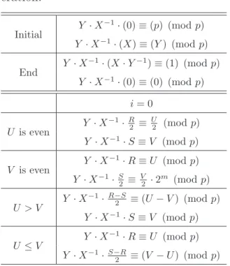
Takagi’s Unified Modular Division Algorithm
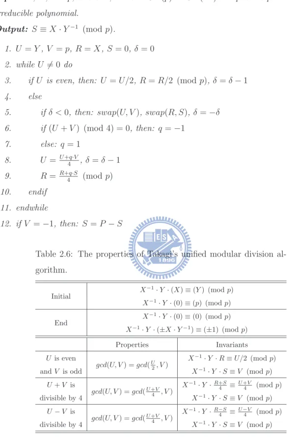
In 1998, Takagi proposed a unified modular division algorithm (T-UMD) [38] based on the extended binary GCD algorithm [57]. The algorithm calculates S = X · Y−1 (mod p) by finding the value gcd(Y, p) and the corresponding modular quotient, where X and Y are the elements of the field with odd prime (or irreducible polynomial) p.
This algorithm requires four operands, U , V , R, and S. U and V are used for cal-culating gcd(Y, p) and the operands R and S are used for calcal-culating modular quotient. The operands U and V are initialized to Y and p, respectively, and the properties shown in Table 2.6 are applied repeatedly to calculate gcd(Y, p). The operands R and S are initialized to the values of X and 0, respectively. Then, the same operations that are
Table 2.5: The properties of Kaliski’s unified inversion algorithm.
Initial X · (0) ≡ −(p) · 2
0 (mod p)
X · (1) ≡ (X) · 20 (mod p)
End of MMI operation X · (−X
−1· 2m) ≡ −(1) · 2m (mod p) X · (0) ≡ (0) · 2ρ (mod p) End of MI operation X · (−X −1) ≡ −(1) (mod p) X · (0) ≡ (0) · 2ρ (mod p) Properties Invariants U is even gcd(U, V ) = gcd(U 2, V )
X · R ≡ −U/2 · 2i+1 (mod p)
X · 2 · S ≡ V · 2i+1 (mod p)
V is even gcd(U, V ) = gcd(U,V 2)
X · 2 · R ≡ −U · 2i+1 (mod p)
X · S ≡ V/2 · 2i+1 (mod p) U > V gcd(U, V ) = gcd(U −V 2 , V ) X · R+S 2 ≡ − U −V 2 · 2 i+1 (mod p) X · 2 · S ≡ V · 2i+1 (mod p)
U ≤ V gcd(U, V ) = gcd(U,V −U 2 )
X · 2 · R ≡ −U · 2i+1 (mod p)
X ·R+S 2 ≡V −U2 · 2 i+1 (mod p) phase 2 – X · R 2 ≡ −(1) · 2i−1 (mod p) X · (0) ≡ (0) · 2ρ (mod p)
ρ is equal to the value i in the last iteration of phase 1.
performed to the operands U and V are applied to the operands R and S for calculating the modular quotient by reducing U and V value. Furthermore, the operands U and V are integers and are allowed to be negative. δ represents α − β, where α and β are values such that 2α and 2β indicate the upper bounds of |U| and |V |, respectively. The value δ = 0 is introduced to represent min(α, β). For correctness, we do some modification on the condition of while loop in the original algorithm.
This algorithm is based on the following invariants: ( X−1· Y · R ≡ U (mod p)
X−1· Y · S ≡ V (mod p)
(2.6)
It can easily be shown that the equivalences always hold in Table 2.6. Since gcd(Y, p) = 1, the operands U = 0 and V is 1 or −1 in the last iteration. Hence, in the final step of algorithm, the equivalence X−1 · Y · S = 1 (mod p) holds and S is equal to X · Y−1 (mod p). Moreover, the number of iterations needed to complete the algorithm is at least m and at most 2m cycles if Y and p are co-prime.
Algorithm 2.8. (Takagi’s unified modular division algorithm.)
Input: X, Y , and p, where X, Y are in GF (p) or GF (2m) and p is the prime integer or irreducible polynomial.
Output: S ≡ X · Y−1 (mod p).
1. U = Y , V = p, R = X, S = 0, δ = 0 2. while U 6= 0 do
3. if U is even, then: U = U/2, R = R/2 (mod p), δ = δ − 1
4. else
5. if δ < 0, then: swap(U, V ), swap(R, S), δ = −δ 6. if (U + V ) (mod 4) = 0, then: q = −1 7. else: q = 1 8. U = U +q·V4 , δ = δ − 1 9. R = R+q·S4 (mod p) 10. endif 11. endwhile 12. if V = −1, then: S = P − S
Table 2.6: The properties of Takagi’s unified modular division al-gorithm. Initial X −1· Y · (X) ≡ (Y ) (mod p) X−1· Y · (0) ≡ (p) (mod p) End X −1· Y · (0) ≡ (0) (mod p) X−1· Y · (±X · Y−1) ≡ (±1) (mod p) Properties Invariants U is even gcd(U, V ) = gcd(U 2, V ) X−1· Y · R ≡ U/2 (mod p)
and V is odd X−1· Y · S ≡ V (mod p)
U + V is gcd(U, V ) = gcd(U +V 4 , V ) X−1· Y ·R+S 4 ≡ U +V 4 (mod p) divisible by 4 X−1· Y · S ≡ V (mod p) U − V is gcd(U, V ) = gcd(U +V 4 , V ) X−1· Y ·R−S 4 ≡ U −V4 (mod p) divisible by 4 X−1· Y · S ≡ V (mod p)
Liu’s Unified Division Algorithm
In algorithm 2.9, the Liu’s unified division algorithm (L-UD) is proposed in [31, 33]. The initial value of U , V , R, and S are set to p, Y , 0, and X, respectively, and the equivalences are shown as follows:
( X−1· Y · R ≡ −U · 2i (mod p)
X−1· Y · S ≡ V · 2i (mod p) (2.7)
The execution cycle of L-UD algorithm is the same as K-UI algorithm, but it can support MMD and MD operations.
Algorithm 2.9. (Liu’s unified division algorithm.)
Input: X, Y , and p, where X, Y are in GF (p) or GF (2m) and p is the prime integer or irreducible polynomial.
Output:
If operation is MMD, then R ≡ X · Y−1· 2m (mod p). If operation is MD, then R ≡ X · Y−1 (mod p). 1. U = p, V = X, R = 0, S = Y , i = 0
2. while V > 0 do
3. if U is even, then: U = U2, S = 2 · S 4. else if V is even, then: V = V2, R = 2 · R
5. else if U − V > 0, then: U = U −V2 , R = R + S, S = 2 · S 6. else if V − U ≥ 0, then: V = V −U2 , S = S + R, R = 2 · R 7. if R ≥ P , then: R = R − p 8. if S ≥ P , then: S = S − p 9. i = i + 1 10. endwhile 11. while i 6= m 0 do 12. if R is even: R = R/2 13. else: R = (R + p)/2 14. i = i − 1 15. endwhile
2.5
Elliptic Curve Cryptographic Applications
ECC can be used to achieve data en/decryption, signature, and authentication [2, 58, 59]. Among them, the major operations are ECSM or the modular division operation.
2.5.1
Elliptic Curve Data En/Decryption
By ECSM operation, the EC data en/decryption [58] can be easy accomplished. We assume that Alice wants to send a message M to Bob. The en/decryption flow is shown in algorithm 2.10.
Algorithm 2.10. (Elliptic Curve Data En/Decryption.)
1. Bob chooses a m-bit random number k as the private key. 2. Bob computes [k]P , then send to Alice.
3. Alice chooses a m-bit random number r.
4. Alice computes {R, S} = {[r]P, M + [r]([k]P )}, then send to Bob. 5. Bob gets the message M by computing S − [k]R.
2.5.2
Elliptic Curve Based Protocols
Many EC based protocols [2, 59], such as elliptic curve digital signature algorithm (ECDSA), EC Menezes-Qu-Vanstone (ECMQV), and EC Diffie-Hellman (ECDH), are used for different applications. For the ECDSA, the domain parameters are given by (H, L, E, N, P ), where H is a hash function, G is a point on the curve of prime order N . Algorithm 2.11 and 2.12 show the ECDSA signing and verification, respectively. Among these two algorithms, the ECSM and MD operations are the most critical.
Algorithm 2.11. (ECDSA signing.)
Input: M , and x, where M is message and k is secret key Output: (R, S), where (R, S) is a signature on M .
1. Choose r ∈ {1, ..., N − 1} 2. T = [r]P
3. R = xT (mod N ), where xT means the x-coordinate of point T 4. if R = 0, then: goto step 1
5. V = H(M )
6. S = (V + kR)/r (mod N ) 7. if s = 0, then: goto step 1
Algorithm 2.12. (ECDSA verification.)
Input: M , Y , G, and (R, S) where M is message, G is public key, and (R, S) is a signature
Output: OU T = Reject or Accept.
1. if R, S /∈ {1, ..., N − 1}, then: OUT = Reject 2. V = H(M ) 3. U1 = V /S (mod N ) 4. U2 = R/S (mod N ) 5. T = [U1]P + [U2]G 6. if R = xT, then: OU T = Accept 7. else: OU T = Reject
2.6
Power Analysis Attacks and Countermeasures
2.6.1
Simple Power Analysis
In most of implementations, the standard sequence of field operations in point addition differs from that in point doubling [4]. The SPA attacks use this difference to reveal the secret key value. In Figure 2.3(a) and 2.3(b), the power traces of the ECDBL and ECADD are shown, respectively. By using the difference between these two trace, the secret key can be revealed. From the power trace of the ECSM operation with secret key in Figure 2.3(c), the key value can be observed.
Several SPA countermeasure methods have been proposed, including unified equation [46], double-and-add-always method [4], and Montgomery ladder [47]. In this work, we adopt double-and-add/sub-always method to accomplish the ECSM operation, which is shown in algorithm 2.13, since the method is easier than the other.
Algorithm 2.13. (Double-and-add/sub-always method.)
Input: P and k, where k is an integer with NAF form and P is a point. Output: Q = [k]P . 1. Q = P 2. for i from m − 2 to 0 by −1 3. Q = [2]Q 4. if ki = 0, then: R = Q + P 5. else if ki = 1, then: Q = Q + P 6. else: Q = Q − P 7. enfor (a) (b) (c) D D D A D A D D
Figure 2.3: (a) A ECADD power trace. (b) A ECDBL power trace. (c) A ECSM power trace.
2.6.2
Differential Power Analysis
In the DPA attacks, an attacker records the power consumption of the cryptographic devices and analyzes the collected power traces by statistical calculation to extract the secret key. Several variations of the DPA attacks have been proposed, such as DPA attack [4], doubling attack [48], address-bit attack [49], refined power analysis [50], and zero-value point attack [51].
Figure 2.4 shows a simple DPA attack flow [33]. The DPA attack assumes that the attacker can perform the ECSM operation with different keys, EC parameters, and EC points, and has knowledge about all the implementation details of the attacked device. For a given secret power trace of ECSM, the attacker reveals the key bit-by-bit. We suppose parts of the secret key [kn−1, kn−2...ki+1] is recognized by the attacker, and the next attacked bit is ki. Next, we input the key-value [kn−1, kn−2...ki+1, ki = 0, ...] and [kn−1, kn−2...ki+1, ki = 1, ...] into the device to obtain two power traces. Then, we cut the traces of [ki = 0] and [ki = 1] from the obtained traces to do further correlation with original power trace. The correlation formula is shown below:
ρ(B, C) = Pli=1(Bi− ¯B)(Ci− ¯C)
√Pl
i=1(Bi− ¯B)2Pli=1(Ci− ¯C)2 (2.8) The parameters B, C mean the l × 1 matrices, and the ρ(B, C) represents the correlation value of B, C, where −1 ≤ ρ ≤ 1. If the correlation between [ki = 0] and original power trace is higher, then the attacker can disclose ki = 0. On the other hand, ki would be 1 if the correlation between the trace for [ki = 1] and that for the original key is higher.
To resist DPA attack, Coron [60] proposed three methods. The Coron’s first coun-termeasure is to randomize the private exponent, such as k′ = k + r · #E(L). Note that the r is a random number, and #E(L) is the curve order. In addition, the second countermeasure is to blind the base point to compute further ECSM, Q = [k]P′ − S, where P′ = P + R, S = [k]R, and R is a random point. The last countermeasure is to randomize a point in projective coordinate. The method changes the original point (x, y, z) to (rx, ry, rz) and performs ECSM in projective coordinate. The security level of a device can be enhanced by increasing the size of random r. Beside, these random methods were classified as the masking DPA countermeasures in [39]. By randomizing the intermediate values that are processed by the cryptographic device, masking method makes the power consumption of a cryptographic device independent of the intermediate values of the cryptographic algorithm to resist the DPA attack.
In [33], a simple DPA attack scheme is used to reveal the secret key from the two chips. The first chip is a 521-bit DECP and the second chip is a 521-bit DECP with PA countermeasure. Coron’s first countermeasure is adopted for DPA countermeasure, since the second method is hard to implement and the third method is only adopted in the projective coordinate. Figure 2.5(a) shows the correlation coefficient trace, and we
can reveal the key value “0”, “0”, “1”, and “0” because the spikes appear in the right locations. On the other hand, in Figure 2.5(b), since there have no spikes in the right locations, the secret key can’t be revealed.
kn-1
Device Original power trace
kn-2 … ki …
Attacked key-bit
kn-1
Guessed power trace 0
kn-2 … 0 …
Assume ki= 0
kn-1
Guessed power trace 1
kn-2 … 1 …
Assume ki= 1
Correlation 0
Correlation 1
Figure 2.4: Simple DPA attack flow
Figure 2.5: Correlation coefficients of key value,[ki = 0, ki−1 = 0, ki−1 = 1, ki−1 = 0], for (a) unprotected chip (b) protected chip.
Chapter 3
Proposed Unified Algorithms
In this chapter, we propose many unified algorithms to support division or multipli-cation operations. In addition, to resist the power analysis attack, the unified random algorithms are proposed.
3.1
Unified Division Algorithm
Traditionally, the FLT is used to achieve the inversion operation in the coordinate and domain transformation. However, the execution cycle is too huge to have the same time complexity with ECSM. Moreover, the K-UI and T-UMD need extra multiplication to achieve the MMD/MD operation. Based on K-UI, we propose a radix-2 unified division (R2-UD) algorithm and a radix-4 unified division (R4-UD) algorithm to reduce numerous execution cycles of division operation.
Table 3.1: The properties of R2-UD.
Conditions Properties U (mod 2) = 0 gcd(U, V ) = gcd(U
2, V )
V (mod 2) = 0 gcd(U, V ) = gcd(U,V 2)
U > V gcd(U, V ) = gcd(U −V 2 , V )
U ≤ V gcd(U, V ) = gcd(U,V −U 2 )
equiva-Table 3.2: The invariant equivalences of the proposed R2-UD algorithm for MMD operation. Initial Y · X −1· (0) ≡ (p) · 20 (mod p) Y · X−1· (X) ≡ (Y ) · 20 (mod p) End Y · X −1· (X · Y−1· 2m) ≡ (1) · 2m (mod p) Y · X−1· (0) ≡ (0) · 2m (mod p) i < m i ≥ m U is even Y · X −1· R ≡ U 2 · 2 i+1 (mod p) Y · X−1·R 2 ≡ U 2 · 2 m (mod p)
Y · X−1· 2 · S ≡ V · 2i+1 (mod p) Y · X−1· S ≡ V · 2m (mod p)
V is even Y · X
−1· 2 · R ≡ U · 2i+1 (mod p) Y · X−1· R ≡ U · 2m (mod p)
Y · X−1· S ≡ V 2 · 2 i+1 (mod p) Y · X−1·S 2 ≡ V 2 · 2 m (mod p) U > V Y · X −1· (R − S) ≡ U −V 2 · 2 i+1 (mod p) Y · X−1·R−S 2 ≡ U −V 2 · 2 m (mod p)
Y · X−1· 2 · S ≡ V · 2i+1 (mod p) Y · X−1· S ≡ V · 2m (mod p)
U ≤ V Y · X
−1· 2 · R ≡ U · 2i+1 (mod p) Y · X−1· R ≡ U · 2m (mod p)
Y · X−1· (S − R) ≡ V −U 2 · 2
i+1 (mod p) Y · X−1·S−R
2 ≡V −U2 · 2
m (mod p)
lences obeyed in our proposed algorithm.
X−1· Y · R ≡ U · 2i (mod p) (3.1)
X−1· Y · S ≡ V · 2i (mod p) (3.2)
For the initialization of R2-UD, the operands U , V , R, and S are set to the values p, Y , 0, and X, respectively. The operations of U V in algorithm 3.1 are based on the binary greatest common divisor (GCD) operation, which is proven in Table 3.1. Note that the addition/subtraction can be implemented by XOR gates in binary field operation and the “1
2” represents “ 1
x”. In each iteration, the valid value of operands U or V is reduced by 1 bits. Because of gcd(U, V ) = gcd(p, Y ) = 1, the values of U and V are 1 and 0 after the last iteration. And the values of R and S are X ·Y−1·2i (mod p) and 0 (mod p), respectively. In addition, the operands R and S are transformed into Montgomery or integer domain due to the MMD or MD operation, respectively. In the beginning of MMD operation, the RS operations are executed to add i by 1. For instance, if the operating step is 19, the equivalences are X−1· Y · (2 · R) ≡ U · 2i+1 (mod p) and X−1· Y · (S − R) ≡ (V −U
2 ) · 2 i+1
(mod p). When i ≥ m, the operations keep the operands R and S in Montgomery domain. In the end of this algorithm, the value R is equal to X · Y−1· 2m (mod p). On the other
Table 3.3: The invariant equivalences of the proposed R2-UD algorithm for MD op-eration. Initial Y · X −1· (0) ≡ (p) (mod p) Y · X−1· (X) ≡ (Y ) (mod p) End Y · X −1· (X · Y−1) ≡ (1) (mod p) Y · X−1· (0) ≡ (0) (mod p) i = 0 U is even Y · X −1·R 2 ≡ U 2 (mod p) Y · X−1· S ≡ V (mod p) V is even Y · X −1· R ≡ U (mod p) Y · X−1· S 2 ≡ V 2 · 2 m (mod p) U > V Y · X −1·R−S 2 ≡ (U − V ) (mod p) Y · X−1· S ≡ V (mod p) U ≤ V Y · X −1· R ≡ U (mod p) Y · X−1·S−R 2 ≡ (V − U) (mod p)
hand, if the operation is set to MD, the data are operated in the integer domain. Then the output value of R is equal to X ·Y−1 (mod p). The detail explanation of the invariant equivalences during the R2-UD is shown in tables 3.2 and 3.3. Besides, Table 3.4 gives an example.
Algorithm 3.2 and 3.3 show the proposed R4-UD and the properties of R4-UD are shown in tabel 3.5. The execution cycle of R4-UD is 0.56m ∼1.12m, since there has a condition reducing just one bit with the probability 18. Consequently, the execution cycle
Table 3.4: The example of the proposed R2-UD.
MMD MD iteration U V R S i U V R S i 1 13 7 0 9 0 13 7 0 9 0 2 3 7 4 5 1 3 7 2 9 0 3 3 2 8 1 2 3 2 2 10 0 4 3 1 3 1 3 3 1 2 5 0 5 1 1 2 2 4 1 1 5 5 0 6 1 0 2 0 4 1 0 5 0 0
Table 3.5: The properties of the proposed R4-UD.
U (mod 4) V (mod 4) Properties 0 0, 1, 2, or 3 gcd(U, V ) = gcd(U
4, V )
1, 2, or 3 0 gcd(U, V ) = gcd(U,V 4)
equivalence gcd(U, V ) = gcd(U −V4 , V ) = gcd(U, V −U 4 ) 2 1 or 3 gcd(U, V ) = gcd( U 2−V 2 , V ) = gcd( U 2, V −U 2 2 ) 1 or 3 2 gcd(U, V ) = gcd(U − V 2 2 , V 2) = gcd(U, V 2−U 2 ) other gcd(U, V ) = gcd(U −V 2 , V ) = gcd(U, V −U 2 )
is 7/8(m/2 ∼ m)+1/8(m ∼ 2m) = 0.56m ∼ 1.12m. The execution cycle of this algorithm is about half the cycles of algorithm 3.1, but the hardware cost is almost two times larger because the total number of RS operations increases from 8 to 21. Consequently, it is an area-time trade-off design.
Compared with previous works, such as FLT-UMMI [26], K-UI [27], and T-UMD [38], our algorithm has fewer execution cycle in division operation without using extra mul-tiplication operation and pre-computed value, 22m. The MMD/MD operating steps and performance analysis is shown in tables 3.6 and 3.7. Moreover, the MMD and MD opera-tions are used many times in ECSM and EC protocols [1], so our design can significantly outperform previous works.
Algorithm 3.1. (Proposed R2-UD algorithm.)
Input: X, Y and p, where X, Y in GF (p) or GF (2m) and p is the prime integer or irreducible polynomial.
Output:
If operation is MMD, then R ≡ X · Y−1· 2m (mod p). If operation is MD, then R ≡ X · Y−1 (mod p). 1. U = p, V = Y , R = 0, S = X 2. if Operation is MMD, then: j = 0 3. else: j = 1 4. while V > 0 do 5. if U is even, then 6. U = U 2
7. if i < m and j = 0, then: S = 2 · S (mod p), i = i + 1
8. else: R = R
2 (mod p) 9. else if V is even, then
10. V = V
2
11. if i < m and j = 0, then: R = 2 · R (mod p), i = i + 1
12. else: S = S
2 (mod p) 13. else if U > V , then
14. U = U −V
2
15. if i < m and j = 0, then: R = R − S (mod p), S = 2 · S (mod p), i = i + 1
16. else: R = R−S
2 (mod p)
17. else
18. V = V −U
2
19. if i < m and j = 0, then: S = S − R (mod p), R = 2 · R (mod p), i = i + 1
20. else S = S−R
2 (mod p)
21. endif
Algorithm 3.2. (Proposed R4-UD algorithm.)
Input: X, Y and p, where X, Y in GF (p) or GF (2m) and p is the prime integer or irreducible polynomial.
Output:
If operation is MMD, then R ≡ X · Y−1· 2m (mod p). If operation is MD, then R ≡ X · Y−1 (mod p). 1. U = p, V = Y , R = 0, S = X 2. while (V > 0) do 3. c = U (mod 4), d = V (mod 4), j = i 4. if i = m − 1, then: ctrl = 1, i = i + 1 5. else if c = 0, then: U = U4, ctrl = 2, i = i + 2 6. else if d = 0, then: V = V 4, ctrl = 3, i = i + 2 7. else if c = d, then 8. i = i + 2 9. if U > V , then: U = U −V4 , ctrl = 4 10. else: V = V −U 4 , ctrl = 5 11. else if c = 2, then 12. i = i + 2 13. if U2 > V , then: U = U 2−V 2 , ctrl = 6 14. else: V = V − U 2 2 , U = U 2, ctrl = 8 15. else if d = 2, then 16. i = i + 2 17. if U > V2, then: U = U − V 2 2 , V = V 2, ctrl = 9 18. else: V = V 2−U 2 , ctrl = 7 19. else 20. i = i + 1 21. if U > V , then: U = U −V2 , ctrl = 10 22. else: V = V −U 2 , ctrl = 11 23. endif 24. (R, S) = OP RS(R, S, ctrl, j, p). 25. endwhile
Algorithm 3.3. (Operations for operands R and S (OP RS).) Input: R, S, ctrl, j and p, where p is an m-bit prime or irreducible poly.. Output: R, S
1. if j < m and operation is MMD, then 2. switch ctrl
3. case 1: R = 2 · R (mod p), S = 2 · S (mod p)
4. case 2: R = 4 · R (mod p)
5. case 3: S = 4 · S (mod p)
6. case 4: R = R − S (mod p), S = 4 · S (mod p) 7. case 5: S = S − R (mod p), R = 4 · R (mod p) 8. case 6: R = R − 2 · S (mod p), S = 4 · S (mod p) 9. case 7: S = S − 2 · R (mod p), R = 4 · R (mod p) 10. case 8: R = 2 · R − S (mod p), S = 4 · S (mod p) 11. case 9: S = 2 · S − R (mod p), R = 4 · R (mod p) 12. case 10: R = R − S (mod p), S = 2 · S (mod p) 13. case 11: S = S − R (mod p), R = 2 · R (mod p)
14. endswitch 15. else 16. switch ctrl 17. case 2: R = R4 (mod p) 18. case 3: S = S4 (mod p) 19. case 4: R = R−S4 (mod p) 20. case 5: S = S−R4 (mod p) 21. case 6: R = R 2−S 2 (mod p) 22. case 7: S = S 2−R 2 (mod p) 23. case 8: R = R− S 2 2 (mod p), S = S 2 (mod p) 24. case 9: S = S− R 2 2 (mod p), R = R 2 (mod p) 25. case 10: R = R−S2 (mod p) 26. case 11: S = S−R2 (mod p) 27. endswitch 28. endif
3.2
Unified Multiplication Algorithm
The traditional method of MMM (i.e. algorithm 2.4) over GF(p) needs one step to recover the value to the range [0, p − 1], but the step is not required in GF(2m) operation. We remove the step by confirming the accumulated operand R always satisfies within the range [0, p − 1]. The overhead is one subtraction. By combining with the proposed UD, the extra units can be shared. In addition, after removing the recover step, the steps of MMM over prime field are similar with that over binary field. Since the proposed UD and MMM are bit-level algorithm, we can combine MM with them to enhance the functionality. Consequently, we propose a 2 unified multiplication (R2-UM) algorithm and a radix-4 unified multiplication (Rradix-4-UM) algorithm shown in algorithms 3.radix-4 and 3.5.
Algorithm 3.4. (Proposed R2-UM.)
Input: X, Y and p, where X, Y are in GF (p) or GF (2m) and p is the prime or irreducible polynomial.
Output:
If Operation is MMM, then R ≡ X · Y · 2m (mod p). If Operation is MM, then R ≡ X · Y (mod p). 1. R = 0, S = Y
2. for i from 0 to m − 1 by +1 do 3. R = R + Xi· S (mod p)
4. if operation is MMM, then: R = R2 (mod p) 5. else: S = 2 · S (mod p)
Algorithm 3.5. (Proposed R4-UM.)
Input: X, Y and p, where X, Y are in GF (p) or GF (2m) and p is the prime or irreducible polynomial.
Output:
If Operation is MMM, then R ≡ X · Y · 2m (mod p). If Operation is MM, then R ≡ X · Y (mod p). 1. R = 0, S = Y
2. for i from 0 to m−1
2 by +1 do
3. if m (mod 2) = 1 and i = m−12 , then: R = R + X2·i· S (mod p) 4. else: R = R + X2·i· S + X2·i+1· 2 · S (mod p)
5. if operation is MMM, m (mod 2) = 1 and i = m−12 , then: R = R2 (mod p) 6. else if operation is MMM, then: R = R
4 (mod p) 7. else: S = 4 · S (mod p)
8. endfor
3.3
Unified Random Algorithms
Based on the masking method, we propose two unified random algorithms to resist DPA attack. We use a m-bit random number r when the modular operations are executed each time. The algorithms have two modes to execute the data operations. The first mode would increase the domain value, and the other would not increase the value. The modes are changed depending on the one in r. When ri is equal to one, the algorithm would execute the first mode, where the value i means the iteration number. Otherwise, the second mode is executed. Consequently, the intermediate value is randomized by the random value r, so the DPA attack can be resisted.
3.3.1
Unified Random Division Algorithm
In algorithm 3.6, the unified random division algorithm (URD) is proposed to support the division operation in random domain, 2λ, where 0 ≤ λ ≤ m. Note that the value λ is equal to the total number of ones in r. The algorithm computes X · Y−1· 2λ (mod p), and have two modes, MMD and MD, to achieve the random domain operation. If ri = 1, the mode is set to MMD to increase the domain value of the operands R and S by 1.
Otherwise, the mode is set to MD which does not increase the domain value. At the end of the algorithm, the output data is in the random domain 2λ.
Algorithm 3.6. (Proposed URD algorithm.)
Input: X, Y , r, and p, where X, Y in GF (p) or GF (2m), r is a random number, and p is the prime integer or irreducible polynomial.
Output: R = X · Y−1· 2λ. 1. U = p, V = Y , R = 0, S = X, λ = 0 2. while V > 0 do 3. if U is even, then 4. U = U 2 5. if ri = 1, then: S = 2 · S (mod p), λ = λ + 1 6. else: R = R 2 (mod p) 7. else if V is even, then
8. V = V 2 9. if ri = 1, then: R = 2 · R (mod p), λ = λ + 1 10. else: S = S 2 (mod p) 11. else if U > V , then 12. U = U −V 2 , 13. if ri = 1, then 14. R = R − S (mod p), S = 2 · S (mod p), λ = λ + 1 15. else: R = R−S2 (mod p) 16. endif 17. else 18. V = V −U 2 19. if ri = 1, then 20. R = 2 · R (mod p), S = S − R (mod p), λ = λ + 1 21. else S = S−R2 (mod p) 22. endif 23. endif 24. endwhile
3.3.2
Unified Random Multiplication Algorithm
Algorithm 3.7 shows the proposed unified random multiplication algorithm (URM) which combines MMM and MM operations to support the multiplication in random do-main, 2λ, where 0 ≤ λ ≤ m. The step 4 is the MMM mode which increases the domain value by 1. And the step 5 is the MM mode which does not change the domain value. Consequently, the value λ is equal to the total number of ones in r.
Algorithm 3.7. (Proposed unified random multiplication algorithm.)
Input: X, Y , p and r, where X, Y are in GF (p) or GF (2m), r is a random number, and p is the prime or irreducible polynomial.
Output: R ≡ X · Y · 2−λ (mod p). 1. R = 0, S = Y , λ = 0 2. for i from 0 to m − 1 by +1 do 3. R = R + Xi· S (mod p) 4. if ri = 1, then: R = R2 (mod p), λ = λ + 1 5. else: S = 2 · S (mod p) 6. endfor
Table 3.6: Operating steps of MMD/MD operations over dual fields of pre-vious works.
FLT
Step MMD MD
1 FLT-UMMI(Y · 2m) = Y−1· 2m (mod p) FLT-UMI(Y ) = Y−1 (mod p)
2 MMM(Y
−1· 2m, X · 2m) MM(Y−1, X)
= X · Y−1· 2m (mod p) = X · Y−1 (mod p)
K-UI
Step MMD MD
1 K-UI(Y · 2m) = Y−1 (mod p) K-UI(Y ) = Y−1· 2m (mod p)
2 MMM(Y −1, X · 2m) MMM(Y−1· 2m, X) = X · Y−1 (mod p) = X · Y−1 (mod p) 3 MMM(X · Y −1, 22m) — = X · Y−1· 2m (mod p) T-UMD Step MMD MD 1 T-UMD(X · 2 m, Y · 2m) T-UMD(X, Y ) = X · Y−1 (mod p) = X · Y−1 (mod p) = X · Y−1 (mod p) 2 MMM(X · Y −1, 22m) — = X · Y−1· 2m (mod p)
Table 3.7: Performance Analysis of Division Operation.
Operation [26] [27] [38] [31] R2-UD R4-UD MMD m2 +m∼2m2 +m 3m∼5m 2m∼3m m∼3m m∼2m 0.56m∼1.12m Execution Time MD m2 +m∼2m2 +m 2m∼4m m∼2m 2m∼4m m∼2m 0.56m∼1.12m Multiplication Operation/
Yes/No Yes/Yes Yes/Yes No/No No/No No/No Pre-computation
Chapter 4
Proposed Architectures
In this chapter, we propose a DECP supporting all the arithmetic functions on elliptic curves over dual fields. Besides, to resist the power analysis attacks, such as SPA, and DPA attacks, we propose a DECP with power analysis countermeasures (DECPAC).
4.1
Galois Field Arithmetic Unit
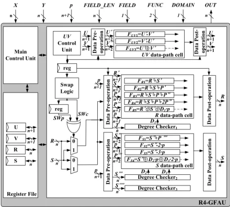
In this section, the radix-2 Galois field arithmetic unit (R2-GFAU) and radix-4 Galois field arithmetic unit (R4-GFAU) are proposed based on the proposed R2-UD/M and R4-UD/M, respectively. These two architectures support all finite field operations, such as MA, MS, MMM, MM, MD, and MMD over dual fields. To increase the operating frequency and reduce the hardware cost, many techniques had been presented. Figures 4.1 and 4.2 are the architectures of R2-GFAU and R4-GFAU. Since the architectures are very similar, only the details of R4-GFAU are illustrated in the following.
In Figure 4.2, the R4-GFAU is controlled by inputs to accomplish the dual-field mod-ular operations. In R4-GFAU, the U V data-path is used to execute the U V operations, and the R, S data-path are used to finish the R, S operations. The following shows an example about the data flow of R4-GFAU. Initially, we set the operation is MMD over GF(p). During the operations, the U V data-path cell compares the two operands (U′,V′)= (U
2,V ) when the operating step is 11. Suppose the decision results are U 2 > V and i < m, and then the (R′,S′,P′,P′′) is set to (2 · R,−S,+p,−p) in R data-path and (S′′,P′′′) is (4 · S,−p) in S data-path to compute the next R, S values. The result of R
is selected from 2R − S + p, 2R − S, 2R − S − p, and 2R − S − 2p in R data-path by deciding whose range is within [0, p − 1]. And the result of S is selected from 4S, 4S − p, 4S − 2p, and 4S − 3p in S data-path. R S D a ta P re -o p er a ti o n D a ta P r e-o p e ra ti o n FS1=S +P R S U V FUV1=U-V FUV2=V-U U V UV Control Unit p p p R S P Main Control Unit R2-GFAU n FS2=S D1·p D1 Degree Checker1 FIELD_LEN 1 FIELD 2 FUNC 1 DOMAIN n+1 p n Y n X n OUT R data-path cell S data-path cell UV data-path cell FR2=R +S +P FR3=R S FR1=R +S +P FUV3=U V D a ta P o st -o p er a ti o n D a ta P o st -o p er a ti o n D a ta P o st -o p e ra ti o n P reg reg 0 1 0 1 SWc SWp Swap Logic P n+1 n+1 n+1 n+1 n+1 n+1 n+1 n+1 n n n+1 n+1 n+1 n+1 Register File U n+1 V n+1 R n S n n n S n S n+1
Figure 4.1: Architecture of R2-GFAU.
4.1.1
Data-path Separation
As the critical path in the proposed R4-UD is from U V path to R, S data-path, a data-path separation method is presented to separate it. The control signal from the U V data-path is stored and sent to RS data-path in the next cycle. Although this approach increases one cycle, the critical path can be reduced from two adders to one adder without considering the data pre-/post-operation. Figure 4.3 shows the detailed flow of the proposed method. Firstly, the U V path is executed. Then, the RS data-path is executed in the next cycle. We can clearly see the data-path is separated and the cycle count is increased by 1.
R S D a ta P re -o p er a ti o n D a ta P r e-o p er a ti o n R S U V D a ta P re -o p er a ti o n F UV1=U -V FUV2=V -U U V UV Control Unit p p p S R S P Main Control Unit R4-GFAU n Degree Checker1 D1 FS4=S D2·p D3·2·p Degree Checker3 D2 D3 Degree Checker2 FIELD_LEN 1 FIELD 2 FUNC 1 DOMAIN n+1 p n Y n X n OUT P R data-path cell S data-path cell UV data-path cell FR3=R +S +P +P FR2=R +S +P FR5=R S D1·p FR1=R +S FUV3=U V D a ta P o st -o p er a ti o n D a ta P o st -o p e ra ti o n D a ta P o st -o p er a ti o n p P reg reg 0 1 0 1 SWc SWp Swap Logic GF(2m) FR4=R +S +P +2P FS3=S -3·p FS2=S -2·p FS1=S +P n+1 U n+1 V n+1 R n S n Register File n+1 n+1 n+1 n+2 n+1 n+2 n+1 n+2 n+1 n+1 n+2 n+2 U V n+1 n+1 n+1 n n n n S S T n n n
Figure 4.2: Architecture of R4-GFAU.
4.1.2
Hardware Sharing
Since both carry-propagation adder and XOR gate are the kernel arithmetic units of every modular operation, we can reuse these addition units to reduce the cost. The detailed hardware sharing method is shown in tables 4.1 and 4.2. The MMD and MM operations require the most adder units in U V , R, and S data-path. And the MA, MS, and MMM operations require only R data-path.
Besides, the division operation requires 21 different operations in R, S data-path. To reduce the hardware complexity, we propose a swap logic circuit. In algorithm 3.3, the operations of value R, S have some common arithmetic operations, such as R = R − 2 · S (mod p) and S = S − 2 · R (mod p) in step 15 and 22. We exploit a swap logic circuit to decide the R, S values are swapped or not in the beginning. The swap operation is decided by the previous and current value of swap signal, SWp and SWc. Note that when the operating step is 3, 4, 6, 8, 10, or 12 in algorithm 3.3, the swap signal is set to 1. Otherwise, the signal value is set to 0. The two operands R, S are swapped when the previous and current swap signals have different values. All the operations of this
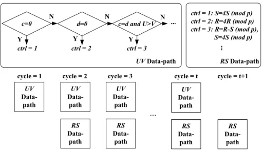
c=d and U>V N Y d=0 c=0 ctrl = 1 ctrl = 2 ... N N Y ctrl = 3 Y UV Data-path ctrl = 1: S=4S (mod p) ctrl = 2: R=4R (mod p) ctrl = 3: R=R-S (mod p), S=4S (mod p) RS Data-path UV Data-path cycle = 1 UV Data-path RS Data-path UV Data-path RS Data-path RS Data-path
cycle = 2 cycle = t cycle = t+1
... UV Data-path RS Data-path cycle = 3
Figure 4.3: Data-path separation method.
algorithm are paired, such as operating steps 4 and 5, 6 and 7, and 8 and 9. By swap logic circuit, the similar operations can be shared and then the number of operations are reduced to 11 types.
In addition, the proposed R4-UD has some common controlled signals between dual fields (e.g., j < m, c = 0, d = 0.), so we can share them to reduce the complexity of controller.
Table 4.1: Details of hardware sharing method in R2-GFAU.
Field Operation FU V 1 FU V 2 FU V 3 FR1 FR2 FR3 FS1 FS2 GF(p) MA/MS X X MMM X X MM X X X X X MMD X X X X X MD X X X X GF(2m) MA X MMM X MM X X MMD X X X MD X X