應用於SVC視訊編碼標準之空間可適性內幀解碼器設計

(1)

國立交通大學

電子工程學系電子研究所碩士班

碩士論文

應用於 SVC 視訊編碼標準之空間可適性內幀解碼器設計

Design of An Intra Predictor with Spatial Scalability

for Scalable Video Decoding

學生：賴昱帆

指導教授：李鎮宜教授

(2)

應用於 SVC 視訊編碼標準之空間可適性內幀解碼器設計

Design of An Intra Predictor with Spatial Scalability

for Scalable Video Decoding

研究生：賴昱帆 Student：Yu-Fan Lai

指導教授：李鎮宜博士 Advisor：Dr. Chen-Yi Lee

國立交通大學

電子工程學系電子研究所碩士班

碩士論文

A Thesis

Submitted to Department of Electronics Engineering & Institute of Electronics College of Electrical and Computer Engineering

National Chiao Tung University in Partial Fulfillment of the Requirements

for the Degree of Doctor of Philosophy in

Electronics Engineering Jul 2009

Hsinchu, Taiwan, Republic of China

(3)

應用於 SVC 視訊編碼標準之空間可適性內幀解碼器設計

學生：賴昱帆指導教授：李鎮宜教授

國立交通大學

電子工程學系電子研究所碩士班

摘要

基於H.264 視訊標準下之可適性視訊壓縮標準(SVC)，是新一代的視訊壓縮規格。與之前的標準相比，在同一種profile 下，SVC 支援了更多的可適性演算法來大大提升視訊的壓縮率。在空間可適性方面，SVC 跟隨著以往多層的演算架構。向量移動補償和內幀預測同樣存在在每一層空間層裡面，就像以往單層的情況一樣。但是，相比較於每一層都是獨立的simulcast 來說，為了要更加提高壓縮的效率，因此在 SVC 中引進了一種層與層之間的預測，這種新加入的方法就叫做層間預測 (Inter-layer Prediction)。 在SVC 的架構當中，特別的是基層(Base Layer)要能夠與傳統 H.264 的標準相符合，並且要能夠解出正確的資料。因此，一個完整的SVC 解碼器不但是要能夠解碼出原來H.264 的位元流，同時也要能夠解碼出 SVC 格式下的位元流。基於上述，我們提出了一個用在high profile SVC 解碼器上的內幀預測架構，而這個架構主要是由兩部分組成：基本內幀預測以及Intra_BL 內幀預測。基本內幀預測是用來處理傳統 H.264 的內幀區塊，在High profile 的規格下，它支援了 macroblock-adaptive frame field (MBAFF)

(4)

的視訊格式，為了減少暫存器的使用量，我們透過重覆使用上方、左方以及角落的暫存器，來優化對圖素的存取，必且提升了存取上面的使用效率。另一個在High profile 下支援的演算法為 Intra_8x8，我們利用提出的 base-mode 預測器來簡化 RSFP (Reference Sample Filtering Process)的過程，同時也優化了暫存器的使用量以及處理的時間。

另一方面，對於處理在SVC 中提供的新內幀預測模式 Intra_BL，我們也提出了另一個預測模組，叫做Intra_BL 內幀預測模組。這個 Intra_BL 內幀預測模組是由 banked SRAM、橫向的基本插補運算單元、縱向的基本插補運算單元以及縱向的延伸式插補運算單元所組成。對於這些插補運算單元，我們也優化了其對面積上面的設計。基於這個初步設計的Intra_BL 內幀預測模組，我們更進一步提出了對於低功率消耗上的改良式低功耗Intra_BL 內幀預測模組設計。主要的改進分為兩部分：第一部分為在原來記憶體階級中，我們加入了第二級暫存器的設計；第二部份為我們利用相等特性來修改了基本插補運算單元的處理流程。加入了這兩種方法，我們可以節省全部功率消耗的46.43%。最後，我們利用90 奈米製程技術實作了整個 SVC 內幀預測架構，跑在頻率為 145 MHz 情況下，總面積為 42756 NAND2 CMOS gates。另外在功率損耗上面，分別跑在頻率為100 MHz 的 H.264 規格下以及頻率為 145 MHz 的 SVC 規格下，功率消耗為 0.292 mW 以及 2.86 mW。而這個設計可以在頻率為 100 MHz 的 H.264 視訊標準下達到每秒30 張 HD1080 的畫面大小，並且可以在頻率為 145 MHz 的 SVC 視訊標準下最大支援到每秒30 張 HD720 和 HD1080 兩層空間層的解碼。

(5)

Design of An Intra Predictor with Spatial Scalability for

Scalable Video Decoding

Student : Yu-Fan Lai Advisor : Dr. Chen-Yi Lee

Department of Electronics Engineering

Institute of Electronics

National Chiao Tung University

ABSTRACT

Scalable Video Coding (SVC) extension of the H.264/AVC is the latest standard in video coding. It has achieved significant improvements in coding efficiency with an increased degree of supported scalability relative to the scalable profiles of prior video coding standards. For supporting spatial scalable coding, SVC follows the conventional approach of multilayer coding. In each spatial layer, motion-compensated prediction and intra-prediction are employed as for single-layer coding. But in order to improve coding efficiency in comparison to simulcasting different spatial resolutions, additional so-called

inter-layer prediction mechanisms are incorporated.

In particular, H.264/AVC compatible bitstream needs to be decoded in the base layer of SVC. Therefore, a SVC decoder must support both traditional H.264 decoding and SVC extension decoding. Specifically, we propose a high profile SVC intra prediction engine

(6)

which is composed of two major prediction modules, basic prediction module and Intra_BL prediction module. Basic prediction module is used to decode the traditional H.264 intra prediction. In order to reduce the buffer size for supporting macroblock-adaptive frame field (MBAFF) coding which is supported in high profile, we optimize the buffer size via upper, left, and corner data reuse sets (DRS) to reuse the pixels and improve the cost and access efficiency. In Luma_8x8 decoding process, we simplify the RSF process via a base-mode predictor and optimize the processing latency and buffer cost.

For the Intra_BL prediction module which is used to decode the new intra prediction type called “Intra_BL”, we propose an Intra_BL prediction engine that consists of banked SRAM, basic horizontal interpolator, basic vertical interpolator and extended vertical interpolator. We also optimize the architecture of interpolators to have better area efficiency than direct implementation. Based on our preliminary Intra_BL prediction module design, we further propose a power efficient Intra_BL prediction module. By applying a second stage of register sets in memory hierarchy and equality determination before basic interpolation process, a total of 46.43% power consumption can be reduced.

Finally, the architecture of this power efficient SVC intra prediction engine is implemented in a 90nm technology with a total area of 42756 NAND2 CMOS gates under working frequency of 145 MHz. The power consumption is 0.292 mW and 2.86 mW under frequency of 100 MHz and 145 MHz for H.264 and SVC, respectively. This design can achieve real-time processing requirement for HD1080 format video in 30fps under the working frequency of 100MHz in H.264, and for a maximum two spatial layers with HD720 and HD1080 scalable format video in 30fps under the working frequency of 145MHz in SVC.

(7)

誌

謝

拿到老師及口試委員們簽名的口試通過單，這一刻我才意識到，我真的畢業了！我非常榮幸能夠在 Si2 實驗室畢業，能夠成為 SI2 的一份子，我真是倍感驕傲。首先我要謝謝這兩年不斷指導我的李鎮宜教授，老師總是用很親切的態度指導我，給了我很多研究上面的觀念，處理、分析問題的方法，以及報告的技巧…等等。雖然老師平常有很多的事要處理，不過老師總是一一回覆每個學生的問題。能跟著老師做研究，不僅是在研究上面有很大的幫助，在做人做事以及平常生活的態度上面，更是有所收穫，謝謝老師！另外要感謝的是蔣迪豪教授，雖然蔣老師平常也忙於公司上面的事情，但是只要老師有控，就會來參加我們group的meeting，並且從業界的角度來給予我們不一樣的建議。還有要感謝我們SI2 的大學長鍾菁哲助理教授，願意抽空回來當我的口委。雖然他目前在中正大學任職，但是學長一直不斷為著SI2 做很多事情。他總是默默付出，如果可以的話真希望學長可以留下來！再來我要感謝帶領我們 multimedia group 的李曜學長，他親切熱心的態度，總是讓我對他充滿感激。不管再小、再基本的問題，他總是很有耐心的指導我。總是把別人的事情放第一，自己放第二的他，是我永遠敬佩的學長。另外也要謝謝同 group 的學長學弟，Mingle、韋罄、阿德、建州、明諭、均宸、浩民、建辰以及昱錚，在我研究之路上給我很多支持以及鼓勵，也帶了很多歡樂給我，謝謝你們！在這也要謝謝其他 SI2 的學長及同學，阿龍、義閔、義澤、建螢、點子、Circus、 Fishya、豪哥、柏均、芳年、小馬、欣儒、智超、耀琳、佳龍，在我遇到問題的時候，總是提供幫助給我，SI2 真是讓人不捨離開的地方！搞不好過幾年我就想回來唸博班了，Kelvin 等我阿，別太早走喔！最後我要謝謝我的家人以及教會的朋友們，每個禮拜回去總是得到很多的關心以及支持，讓我能夠充滿精神開始下禮拜的研究。這一切的一切，有太多說不完的感謝，感謝上帝！

(8)

List of Figures

FIGURE 1: THE CONTAINED TECHNIQUES IN DIFFERENT PROFILES OF H.264/AVC STANDARD. ... 5

FIGURE 2: BLOCK DIAGRAM OF H.264/AVC VIDEO ENCODER. ... 8

FIGURE 3: BLOCK DIAGRAM OF H.264/AVC VIDEO DECODER. ... 8

FIGURE 4: INTRA_4X4 PREDICTION MODE DIRECTIONS. ... 9

FIGURE 5: INTRA_4X4 PREDICTION MODES BASED ON THE NEIGHBORING PIXELS. ... 10

FIGURE 6: INTRA_16X16 PREDICTION MODES BASED ON THE NEIGHBORING PIXELS. ... 10

FIGURE 7: (A) A MB PAIR WHICH IS CODED IN FRAME MODE AND FIELD MODE, AND (B) AN EXAMPLE OF DIFFERENT COMBINATIONS OF MB PAIRS IN A PICTURE. ... 12

FIGURE 8: (A) SCANNING ORDER IN DIFFERENT DECODING UNITS OF A FRAME AND (B) RELATIONSHIP BETWEEN CURRENT UNIT AND NEIGHBORING UNITS ... 13

FIGURE 9: PSNR VS BIT RATE CURVE FOR THE (A) MOBILE SEQUENCE AND (B) STEFAN SEQUENCE. ... 14

FIGURE 10: NEIGHBORING INFORMATION IN (A) FRAME MODE MB PAIR AND (B) FIELD MODE MB PAIR (ASSUME NEIGHBORING MB PAIRS ARE ALL CODED IN FRAME MODE). ... 15

FIGURE 11: DIFFERENCE BETWEEN INTRA_8X8 AND INTRA_16X16/INTRA_4X4 ... 16

FIGURE 12: NINE INTRA_8X8 PREDICTION MODES (NOTE: EACH NEIGHBORING PIXEL (A~Y) IS ALREADY FILTERED BY RSFP). ... 16

FIGURE 13: SVC ENCODER BLOCK DIAGRAM (NOTE: ENHANCEMENT LAYER CAN BE MORE THAN 1). ... 20

(12)

FIGURE 15: POSSIBLE INTER-LAYER PREDICTION PROCESS SUPPORTED IN SVC. ... 24

FIGURE 16: INTRA PREDICTION TYPES IN BASE LAYER AND ENHANCEMENT LAYER. ... 25

FIGURE 17: BLOCK DIAGRAM OF INTRA_BL DECODING PROCESS. ... 26

FIGURE 18: BLOCK DIAGRAM OF SVC INTRA PREDICTION ENGINE. ... 27

FIGURE 19: BLOCK DIAGRAM OF THE PROPOSED H.264 HIGH-PROFILE INTRA PREDICTOR. ... 29

FIGURE 20: MEMORY HIERARCHY OF H.264 HIGH-PROFILE INTRA PREDICTOR. ... 30

FIGURE 21: THE UPDATED DIRECTION OF UPPER/LEFT BUFFER MEMORY IN (A) FRAME AND (B) FIELD MODE MB PAIR. ... 31

FIGURE 22: LINE SRAM DATA_OUT REPLACES THE LAST SUB-ROW OF UPPER BUFFER. ... 32

FIGURE 23: THE UPDATED DIRECTION OF CORNER PIXEL BUFFERS. ... 34

FIGURE 24: THE PIPELINE SCHEME OF MBAFF DECODING. ... 35

FIGURE 25: INTRA PREDICTOR IN [14]. ... 36

FIGURE 26: INTRA PREDICTOR IN [19]. ... 37

FIGURE 27: MODIFIED BASE-MODE INTRA PREDICTOR. ... 37

FIGURE 28: ARCHITECTURE OF AN INTRA 8×8 DECODING MODULE. ... 38

FIGURE 29: BEHAVIOR OF SHARED FILTER. ... 39

FIGURE 30: PROPOSED INTRA_BL PREDICTION DECODING BLOCK DIAGRAM. ... 42

FIGURE 31: SVC DECODER SYSTEM BLOCK DIAGRAM. ... 43

FIGURE 32: ANALYSIS OF POWER DISSIPATION ON EXTERNAL SDRAM AND INTERNAL SRAM. . 44

FIGURE 33: BANKED SRAM AND REQUIRED REGION FOR DIFFERENT PICTURE TYPE PREDICTIONS BETWEEN SPATIAL LAYERS. ... 45

FIGURE 34: UPDATING PROCESS OF BANKED SRAM. ... 46

FIGURE 35: PROPOSED ARCHITECTURE OF BASIC INTERPOLATOR. ... 48

FIGURE 36: THE ARCHITECTURE OF CHROMA COEF_GENERATOR. ... 49

(13)

GENERATES THREE SCALED SETS. ... 51

FIGURE 39: THE ARCHITECTURE OF (A) SCALING_ENGINE1 AND (B) SCALING_ENGINE2. ... 52

FIGURE 40: PROPOSED ARCHITECTURE OF EXTENDED VERTICAL INTERPOLATOR. ... 53

FIGURE 41: DIRECT IMPLEMENTATION OF BASIC INTERPOLATOR. ... 54

FIGURE 42: INTRA POWER CONSUMPTION IN H.264/AVC AND SVC. ... 57

FIGURE 43: POWER ORGANIZATION OF INTRA_BL PREDICTION ENGINE. ... 57

FIGURE 44: MEMORY HIERARCHY IMPROVEMENT OF INTRA_BL PREDICTION ENGINE. ... 58

FIGURE 45: SOME DEFINITIONS OF REPRESENTATIONS. ... 59

FIGURE 46: AN EXAMPLE OF USING THESE REGISTER SETS. ... 60

FIGURE 50: MODIFIED INTRA_BL DECODING PROCESS. ... 66

FIGURE 51: PROPOSED POWER EFFICIENT INTRA_BL PREDICTION ENGINE. ... 66

FIGURE 52: POWER REDUCTION OF PROPOSED DESIGN. ... 68

FIGURE 53: (A) ONE-TO-FOUR METHOD AND (B) UPSAMPLING METHOD IN SVC FOR TEST SEQUENCE “GLASGOW”. ... 72

FIGURE 54: (A) ONE-TO-FOUR METHOD AND (B) UPSAMPLING METHOD IN SVC FOR TEST SEQUENCE “SUZIE”. ... 73

(14)

List of Tables

TABLE 1: CODING TOOLS IN DIFFERENT PROFILES OF H.264/AVC STANDARD ... 6

TABLE 2: CODING TOOL DIFFERENCE BETWEEN SVC PROFILES ... 19

TABLE 3: INTERPOLATION COEFFICIENTS FOR LUMA AND CHROMA UP-SAMPLING. ... 26

TABLE 4: NUMBER OF FILTERED PIXELS ACTUALLY NEEDED IN INTRA 8X8 MODES. ... 36

TABLE 5: AVERAGE CYCLES NEEDED FOR DECODING A MB IN DIFFERENT VIDEO SEQUENCES. ... 39

TABLE 6: COMPARISON RESULTS. ... 40

TABLE 7: CHROMA TABLE IN BINARY FORM. ... 49

TABLE 8: LUMA TABLE IN BINARY FORM. ... 50

TABLE 9: SIMULATION RESULTS OF PROPOSED BASIC INTERPOLATOR AND EXTENDED VERTICAL INTERPOLATOR. ... 54

TABLE 10: INTERPOLATION EXECUTION TIME FOR A MB IN WORST CASE. ... 55

TABLE 11: PROPOSAL DESCRIPTION. ... 56

TABLE 12: SRAM POWER REDUCTION BY FOUR REGS SETS. ... 64

TABLE 13: PROCESSING CYCLE REDUCTION BY FOUR REGS SETS (FRAME - MBAFF). ... 64

TABLE 14: PROPERTY OF COEFFICIENT SETS IN LUMA AND CHROMA FILTER TABLES. ... 65

TABLE 15: COMPARISONS BETWEEN NEW PROPOSAL AND PRELIMINARY DESIGN. ... 67

TABLE 16: PROBABILITIES OF EQUALITY IN DIFFERENT QPS AND TEST SEQUENCES. ... 67

(15)

Chapter 1 Introduction

1.1 Motivation

H.264/AVC [1]-[2] is the latest international video coding standard from MPEG and ITU-T Video Coding Experts Group. It consists of three profiles which are defined as a subset of technologies within a standard usually created for specific applications. Baseline and main profiles are intended as the applications for video conferencing/mobile and broadcast/storage, respectively. Considering the H.264-coded video in high profile, it targets on the compression of high-quality and high-resolution video and becomes the mainstream of high-definition consumer products such as HD DVD and Blu-ray disc. However, high-profile video is more challenging in terms of implementation cost and access bandwidth since it involves extra coding engine, such as macroblock-adaptive frame field (MBAFF) coding (using a macroblock pair structure for pictures coded as frames, allowing 16×16 macroblocks in field mode) and Luma 8×8 intra coding, for achieving high performance compression.

On the other hand, considering that future applications will support a different range of display resolutions and transmission channel capacities, the Joint Video Team (JVT) has developed a scalable extension [3]-[4] based on the state-of-the-art H.264/AVC standard which was completed in November 2007. This extension is commonly known as Scalable Video Coding (SVC), and it provides multiple display resolutions within a single compressed bit-stream, which is referred to spatial scalability in SVC. Additionally, the SVC extension supports combinations of temporal scalability (frame rate) and quality scalability (fidelity enhancement under the same resolution) with the spatial scalability feature. This is achieved while balancing both decoder complexity and coding efficiency.

(16)

The need for spatial scalability is motivated by the resolutions variety of current display devices. Specifically, larger format, high definition displays are becoming commonly used in consumer applications, with displays containing over two million pixels. By contrast, lower-resolution displays with between ten thousand and one hundred thousand pixels are also popular in applications due to the considerations of size, power, and weight. However, transmitting a single representation of a video sequence to the different of display resolutions in the market is impractical. For example, it is rarely reasonable to design a device with low display resolution with the capacity for decoding and downsampling high-resolution video sequence. This kind of requirement could increase the cost and power of the device in order to determine its display resolution. In addition, it may be a waste of channel capacity to send the high-resolution video bitstreams that are ultimately not shown on the display for such a device.

Therefore, the new scalable extension of H.264 standard can not only support multiple resolutions decoding but also provide better compression compared to the prior standards. Furthermore, considering that the overall complexity and other overheads will be increased in SVC, the proposed methods can be efficient to reduce the area, computational complexity, and power consumption.

1.2 Thesis Organization

This thesis is organized as follows. In Chapter 2, the intra prediction process in different profiles and some important coding tools which for achieving high performance compression will be described. For the additional features in intra prediction of SVC such as spatial scalability, new prediction mode and inter-layer intra prediction between different video types (progressive or interlace) will also be introduced. Then, the architecture design and implementation results of intra prediction engine which supports H.264/AVC high profile and

(17)

scalable extension will be shown in Chapter 3 and Chapter 4, respectively. Finally, the conclusions and future works will be presented in Chapter 5.

(18)

Chapter 2 Overview the Intra Prediction in

H.264/AVC and Scalable Video Coding

2.1 H.264/AVC Standard Overview

H.264/AVC is the newest international video coding standard from MPEG and ITU-T Video Coding Experts Group. It provides various kinds of powerful but complex techniques to achieve higher video compression, such as spatial prediction in intra coding, adaptive block-size motion compensation, 4×4 integer transformation, context-adaptive entropy coding, adaptive deblocking filtering, and etc.

2.1.1 Profiles and Levels

In order to achieve different specific classes of applications, the standard includes the following profiles. We take four commonly used profiles to be described.

 Baseline Profile: This profile is used widely for lower-cost applications with limited computing resources, such as in videoconferencing and mobile applications.

 Main Profile: Intended as the mainstream consumer profile for broadcast and storage applications. However, the importance of this profile is faded when the high profile was developed for those applications.

 Extended Profile: This profile is intended for the streaming video profile, and has relatively high compression capability and some extra methods for robustness to error and server stream switching.

(19)

particularly for high-definition television applications (for example, HD DVD and Blu-ray Disc).

Figure 1 shows the difference between coding techniques in different profiles of H.264/AVC standard. To be noticed, the coding tools “Interlace” and “8x8 Integer DCT” in Main and High profiles are referred to the Macroblock-Adaptive Frame-Field (MBAFF) coding (or Picture-Adaptive Frame-Field (PAFF) coding) and Luma Intra_8x8 prediction mode.

Figure 1: The contained techniques in different profiles of H.264/AVC standard.

These two additional coding tools can further increase the performance of compression. PAFF and MBAFF was reported to reduce bit rates in the range of 16 to 20% and 14 to 16% over frame-only and PAFF for ITU-R 601 resolution sequences like “Canoa” and “Mobile and Calendar”, respectively [2]. Moreover, Intra_8x8 supports more options to predict the block, and provides more efficient compression than Intra_4x4 and Intra_16x16 only. For more details about coding tool difference are listed in Table 1.

(20)

Table 1: Coding tools in different profiles of H.264/AVC standard

Coding Tools Baseline Main Extend High

I and P Slices Yes Yes Yes Yes

B Slices No Yes Yes Yes

SI and SP Slices No Yes No No Multiple Reference Frames Yes Yes Yes Yes

In-Loop Deblocking Filter Yes Yes Yes Yes

CAVLC Entropy Coding Yes Yes Yes Yes

CABAC Entropy Coding No No Yes Yes

Flexible Macroblock Ordering (FMO) Yes Yes No No Arbitrary Slice Ordering (ASO) Yes Yes No No Redundant Slices (RS) Yes Yes No No Data Partitioning No Yes No No Interlaced Coding (PicAFF, MBAFF) No Yes Yes Yes

4:2:0 Chroma Format Yes Yes Yes Yes

Monochrome Video Format (4:0:0) No No No Yes

4:2:2 Chroma Format No No No No 4:4:4 Chroma Format No No No No 8 Bit Sample Depth Yes Yes Yes Yes

9 and 10 Bit Sample Depth No No No No 11 to 14 Bit Sample Depth No No No No 8x8 vs. 4x4 Transform Adaptivity No No No Yes

Quantization Scaling Matrices No No No Yes

Separate Cb and Cr QP control No No No Yes

(21)

Predictive Lossless Coding No No No No

2.1.2 Encoder/Decoder Block Diagram

As mentioned before, H.264/AVC standard provides much higher video compression performance by some new coding tools. However, the complexity is also increased. Figure 2 shows the block diagram of H.264/AVC video encoder. An embedded decoder exists inside the encoder that calculates the motion compensation and intra prediction at the decoder side. With this embedded decoder in the encoder side, the encoder can foresee the decoded result and precisely calculate the residual pixel values without mismatch to the decoder. One of the major differences compared to previous standard is the intra prediction in H.264/AVC standard. Several prediction modes are provided for the intra prediction to highly improve the compression ability in the spatial domain. On the other side, the motion compensation supports variable block sizes, multiple reference frames, and short/long term prediction to reduce the redundancy in the temporal domain. After subtracting the input video with the predicted pixels which are from the intra prediction or motion compensation, the residual values are processed with DCT, quantization and entropy coding to reduce the coding redundancy. Moreover, H.264/AVC uses powerful block-based compression methods to increase the performance. However, another problem called “blocky effect” will be generated. In order to solve this problem, H.264 uses the in-loop filter, deblocking filter, to improve the visual quality. Finally, the coded bit stream is produced and transmitted.

On the decoder side, it lacks of the decision parts like motion estimator and the intra mode decision parts. Hence, the decoder is simpler than the encoder. Figure 3 shows the block diagram of H.264/AVC video decoder. After entropy decoding the input bit stream, the syntax elements are decoded to decide which mode is used in motion compensation or intra prediction. Then, the residual values are generated by inverse quantization and IDCT. With

(22)

residual values and predicted pixel values, the video can be constructed. Finally, the deblocking filter is invoked to eliminate the blocky effects and improve the visual quality.

Figure 2: Block diagram of H.264/AVC video encoder.

Figure 3: Block diagram of H.264/AVC video decoder.

(23)

As shown in Figure 3, the intra prediction (the grey block) is one of the major prediction engines in H.264/AVC standard. In the previous section, we have mentioned about that H.264 provides several prediction modes in intra prediction to improve the compression ability in the spatial domain. There are two classes of intra prediction modes in baseline and main profile of H.264/AVC, the Intra_4x4 prediction mode and Intra_16x16 prediction mode. Besides, the third class of intra prediction called Intra_8x8 which is supported in high profile will be further introduced in Section 2.1.5.

Figure 4: Intra_4x4 prediction mode directions.

There are a total of 9 optional prediction modes for Intra_4x4 prediction mode. The arrows in Figure 4 indicate the direction of prediction in each mode. These 9 modes are vertical (0), horizontal (1), DC (2), diagonal down-left (3), diagonal down-right (4), vertical-right (5), horizontal-down (6), vertical-left (7), and horizontal-up (8), respectively.

The prediction 4x4 blocks (which are grey color in Figure 5) are calculated based on the neighboring samples labeled A-M in Figure 5, as follows. In DC modes, the intra prediction process is to calculate the mean value of neighboring pixel values. Except for DC mode, all the others are calculated by four neighboring pixel values. These four pixels are different according to the type of mode and the position in the 4x4 block.

(24)

Figure 5: Intra_4x4 prediction modes based on the neighboring pixels.

In the Intra_16x16 prediction mode class, there are a total of 4 optional prediction modes, which are vertical, horizontal, DC, and plane modes, as shown in Figure 6, respectively. The vertical, horizontal, and DC modes are very similar to the Intra_4x4 prediction modes described before. The new prediction mode in Intra_16x16 is plane mode, which is a “linear” plane function that is fitted to the upper and left-hand samples H and V. This works well in areas of smoothly-varying luminance.

(25)

For a luma samples in a macroblock, both Intra_4x4 prediction modes and Intra_16x16 prediction modes are valid. However, only 4 prediction modes which are very similar to the 16x16 luma prediction modes but with a little different in parameters are valid in chroma samples.

2.1.4 Macroblock-Adaptive Frame-Field Intra Decoding

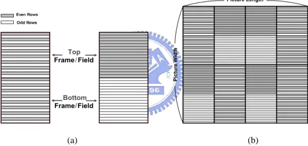
There usually exist two types of video source formats, i.e. progressive and interlaced video, for which different techniques were presented in a range of video standards, such as H.261 [5], H263 [6], MPEG-1 [7], MPEG-2 [8], and MPEG-4 [9] as well as in H.264/AVC [1] a newly released standard. In particular, a frame of interlace video sequence consists of two fields, scanned at different time instants. Therefore, a video sequence consisting of interlaced video can be compressed in many different ways. They can be grouped in two main categories: (a) Fixed Frame/Field and (b) Adaptive Frame/Field.

2.1.4.1 Types of Video Source Formats

In the first category, all the frames of a sequence are encoded in either frame or field mode. In the second category, depending on the content, one adaptively selects whether to use the field or frame structure. Adaptation can be done at either picture level or macroblock level. For the picture level adaptation of frame/field (PAFF), an input frame of a sequence can be encoded as one frame or two fields. If frame mode is chosen, a picture created by interleaving both even number pixels and odd number pixels is partitioned into some 16x16 macroblocks (MBs) and coded as a whole frame. However, in field coding, the top and bottom field pictures are partitioned into 16x16 MBs and coded as separate pictures. For MB level adaptation of frame/field coding (MBAFF), the frame is partitioned into 16x32 MB pairs, and the two MBs in each MB pair are both coded in frame mode or field mode, as shown in

(26)

Figure 7(a). Further, any combinations of MB pairs can also exist in a picture, as illustrated in Figure 7(b) (In Figure 7, we assume that picture length and width are both 64 pixels).

Therefore, there exist two decoding units according to the video source format. One is called MB in fixed frame/field video source format and picture level adaptive frame/field video source format, and the other is called MB pair in MBAFF video source format. The sizes of MB and MB pair are 16x16 and 16x32, respectively. The scanning order in different decoding units of a frame and the relationship between current unit and neighboring units are described in Figure 8(a) and Figure 8(b).

(a) (b)

Figure 7: (a) A MB pair which is coded in frame mode and field mode, and (b) an example of different combinations of MB pairs in a picture.

In a short summary about video sequence formats, it is believed that frame coding is more efficient than field coding for progressive video and static pictures in interlaced video, while field coding is more efficient for moving pictures in interlaced video. Thus, picture-adaptive frame/field (PAFF) coding is supported in H.264 to improve the coding efficiency for interlaced video with both static and moving pictures. Obviously, PAFF coding requires the encoder has the ability to adaptively select the picture coding mode, which is

(27)

realized by 2-pass coding in reference software of H.264, i.e., frame mode and field mode are performed respectively, and the one with smaller rate-distortion cost is chosen as the optimal picture coding mode.

(a)

(b)

Figure 8: (a) Scanning order in different decoding units of a frame and (b) relationship between current unit and neighboring units

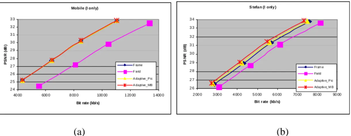
As an extension of PAFF, MBAFF is used to improve coding efficiency of picture with both static and moving regions. Reference software performs MBAFF coding with a 2-pass coding strategy on MB pair level. Every MB pair is coded in frame mode and field mode respectively, and the mode with smaller rate-distortion cost is selected. In general, MBAFF coding is more efficient for video coding. Figure 9 gives some simulation result about different video sequence formats in different test sequences [10].

(28)

Mobile (I only) 2 4 2 5 2 6 2 7 2 8 2 9 3 0 3 1 3 2 3 3 40 00 600 0 8 00 0 100 00 1 20 00 1 400 0 Bit rate (kb/s) PSN R (d B ) F rame F ield A dapt ive_P ic A dapt ive_MB S tefa n (I only ) 2 6 2 7 2 8 2 9 3 0 3 1 3 2 3 3 3 4 2 00 0 3 00 0 4 00 0 5 0 00 6 0 00 70 00 80 00 90 00 Bit r ate (kb/s) PS N R (d B ) Fram e Field Adaptiv e_P ic Adaptiv e_M B (a) (b)

Figure 9: PSNR vs bit rate curve for the (a) Mobile sequence and (b) Stefan sequence.

2.1.4.2 Intra Block Neighboring Information in MBAFF

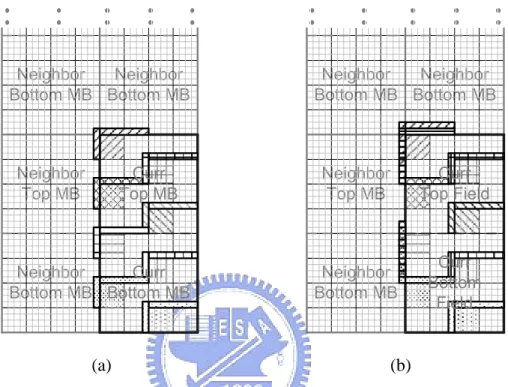
As mentioned in the previous section, the even rows and odd rows will be gathered to different MBs (top or bottom MB in a MB pair) according to the different modes of a MB pair. Therefore, the neighboring pixels of an intra block will also be more complex when the MBAFF is supported.

Figure 10 shows the neighboring pixels of a 4x4 intra block in the MB pair. When the current MB pair is coded in frame mode, the neighboring pixels are similar to the baseline profile which has the unit in MB, as illustrated in Figure 10 (a). However, when the current MB pair is coded in field mode, the relationship between current 4x4 block and neighboring pixels will be more complicated, and the neighboring pixels are no more around to a 4x4 block. Depending on the 4x4 blocks in a MB pair, the neighboring pixels will be in different positions, as shown in Figure 10 (b). In a simple way to express the principle about neighboring pixels is that the pixels in top (or bottom) field of current block can only find the neighboring pixels also in top (or bottom) field of neighboring blocks. Besides, if neighboring blocks are not coded in field mode, the first step is to convert the frame mode block into field block. Then, find the corresponding neighboring pixels in the same field. Furthermore, there

(29)

are a total of 4 cases between current MB pair and neighboring MB pair (frame/frame, frame/field, field/frame, and field/field). Here we just take 2 cases (frame/frame and frame/field) for an example.

(a) (b)

Figure 10: Neighboring information in (a) frame mode MB pair and (b) field mode MB pair (assume neighboring MB pairs are all coded in frame mode).

Obviously, in order to support MBAFF mode, it needs more side information to indicate the frame/field mode of each MB pair. Therefore, how to efficiently store and decode these neighboring pixels and MB pairs becomes an important issue in MBAFF video format.

2.1.5 Intra_8x8 Prediction Mode Decoding

For intra prediction, luma Intra_8x8 is an additional intra block type supported in H.264 high profile which supports all features of the prior main profile. The luma Intra_8x8 prediction is introduced by extending the concepts of Intra_4x4 prediction but with an additional process as described in Figure 11.

(30)

Figure 11: Difference between Intra_8x8 and Intra_16x16/Intra_4x4

Figure 12: Nine Intra_8x8 prediction modes (note: each neighboring pixel (A~Y) is already filtered by RSFP).

Similar to Intra_4x4, Intra_8x8 has nine different direction prediction modes, as shown in Figure 12. The luma values of each sample in a given 8x8 block are predicted from neighboring reconstructed reference pixels base on prediction modes. It should be noticed that before decoding an Intra_8x8 block, there is an extra process that is different from Intra_4x4

(31)

be filtered first, and then using these filtered pixels to predict subsequent 8×8 blocks. For an

Intra_4x4 and Intra_8x8 block, 13 neighbors and 25 filtered neighbors are needed,

respectively.

This new intra coding tool not only improves I-frame coding efficiency significantly [11], but also induces some extra cycles and data dependency in order to generate the filtered neighboring pixels.

2.2 SVC Extension of H.264/AVC Standard Overview

Scalable Video Coding (SVC) [12] is the name given to an extension of the H.264/AVC video compression standard. SVC enables the transmission and decoding of partial bit streams to provide video services with lower temporal or spatial resolutions or reduced fidelity while retaining a reconstruction quality that is high relative to the rate of the partial bit streams. Hence, SVC provides some techniques such as graceful degradation in lossy transmission environments, bit rate, format, and power adaptation. By these techniques, SVC can enhance the transmission and storage within applications. Furthermore, SVC has achieved significant improvements in coding efficiency with an increased degree of supported scalability relative to the scalable profiles of prior video coding standards.

Scalable Video Coding as specified in extension of H.264/AVC allows the construction of bitstreams that contain sub-bitstreams which conform to H.264/AVC. For temporal bitstream scalability, it provides the presence of a sub-bitstream with a smaller sampling rate than the bitstream. When deriving the temporal sub-bitstream, complete access units will be removed from the bitstream. For spatial and quality bitstream scalability, these two scalabilities provide the presence of a sub-bitstream with lower spatial resolution or quality than the bitstream. When deriving these kinds of sub-bitstream, the NAL (Network Abstraction Layer) will be removed from the bitstream. In this case, inter-layer prediction (i.e.

(32)

the prediction between the higher spatial resolution or quality layer and the lower spatial resolution or quality layer) is typically used for improving the coding efficiency, and will be more explained in Section 2.2.2.

2.2.1 Profiles and Levels

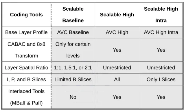
As a result of the Scalable Video Coding extension [13], the standard contains three additional scalable profiles: Scalable Baseline, Scalable High, and Scalable High Intra. These profiles are defined as a combination of the H.264/AVC profile for the base layer and tools that achieve the scalable extension:

 Scalable Baseline Profile: Primarily targeted for mobile broadcast, conversational and surveillance applications that require a low decoding complexity. In this profile, the support for spatial scalable coding is restricted to resolution ratios of 1.5 and 2 between spatial layers in both horizontal and vertical direction and to macroblock-aligned cropping. Furthermore, the coding tools for interlaced sources are not included in this profile. Bit streams conforming to the Scalable Baseline profile contain a base layer bit stream that conforms to the restricted Baseline profile H.264/AVC. It should be noted that the Scalable Baseline profile supports B slices, weighted prediction, the CABAC entropy coding, and the 8x8 luma transform in enhancement layers (CABAC and the 8×8 transform are only supported for certain levels), although the base layer has to conform to the restricted Baseline profile, which does not support these tools.

 Scalable High Profile: Primarily designed for broadcast, streaming, and storage applications. In this profile, the restrictions of the Scalable Baseline profile are removed and spatial scalable coding with arbitrary resolution ratios and cropping parameters is supported. Bit streams conforming to the Scalable High profile contain a base layer bit stream that conforms to the High profile of H.264/AVC.

(33)

 Scalable High Intra Profile: Primarily designed for professional applications. Bit streams conforming to this profile contain only IDR pictures (for all layers). Besides, the same set of coding tools as for the Scalable High profile is supported.

The coding tool differences between SVC profiles are described in Table 2.

Table 2: Coding tool difference between SVC profiles

Coding Tools Scalable Baseline Scalable High Scalable High Intra

Base Layer Profile AVC Baseline AVC High AVC High Intra CABAC and 8x8

Transform

Only for certain levels

Yes Yes

Layer Spatial Ratio 1:1, 1.5:1, or 2:1 Unrestricted Unrestricted I, P, and B Slices Limited B Slices All Only I Slices

Interlaced Tools (MBaff & Paff)

No Yes Yes

2.2.2 Encoder/Decoder Block Diagram

The example for combining spatial, quality, and temporal scalabilities is illustrated in Figure 13, which shows an encoder block diagram with two spatial layers.

The SVC coding structure is organized in dependency layers (i.e. spatial layers). A dependency layer usually represents a specific spatial resolution, and is identified by a layer identifier, D. The identifier D equals 0 for the base layer which is also a H.264/AVC compatible layer, and it is increased by 1 from one spatial layer to the next. For each dependency layer, the basic prediction engine of motion compensation and intra prediction in H.264 are used as in single-layer coding. Further, the additional inter-layer prediction which

(34)

is exploited to reduce the redundancy between dependency layers will be more explained in Section 2.2.3.1. Hence, by applying this new inter-layer prediction in SVC, the coding efficiency related to spatial scalability provides higher coding efficiency than the simulcasting between different spatial resolutions.

Figure 13: SVC encoder block diagram (note: enhancement layer can be more than 1).

In a special case that the spatial resolutions for two dependency layers are identical, in which case the different layers provide coarse-grain scalability (CGS) in terms of quality. However, this multilayer concept for quality scalable coding only allows a few selected bit rates to be supported in a scalable bit stream. Therefore, in order to increase the flexibility of bit stream adaptation and error robustness, but also for improving the coding efficiency for bit streams that have to provide a variety of bit rates, an extension of the CGS approach, which is also referred to as medium-grain quality scalability (MGS), is included in the SVC design. The difference between CGS and MGS are a modified high level signaling, which allows a switching between different MGS layers in any access unit. Finally, these scalable

(35)

sub-streams will be organized to a scalable bit stream and transmitted.

Figure 14: SVC decoder block diagram with two spatial layers.

The block diagram of SVC decoder is similar to Figure 3 in Section 2.1.2, but with some additional processes for enhancement layer decoding. When the base layer is decoding, the overall decoding flow is the same as H.264/AVC decoding flow. However, there are some additional processes chosen for decoding the enhancement layers. The block diagram of SVC

(36)

decoder with two spatial layers is shown in Figure 14.

For spatial enhancement layers, SVC includes a new macroblock type which is involved by inter-layer prediction. For this macroblock type, only a residual signal but no additional side information such as intra prediction modes or motion parameters is transmitted. In intra prediction, the new prediction mode “I_BL” provides an additional prediction source for the scalable enhancement layer. When this new prediction mode I_BL is used in enhancement layer, the decoder will perform the following two major steps. First, it decodes the co-located blocks in the lower-resolution layer and applies a deblocking filter. Then, upsampling these samples of the lower resolution layer to form a prediction. On the other hand, the partitioning information of the enhancement layer macroblock, reference indices, and motion vectors are derived from the corresponding information of the co-located block in the reference layer for motion compensation. Furthermore, residual information of inter-picture coded MBs from a lower resolution layer can also be used for the prediction of the residual in the enhancement layer. The lower resolution layer residuals of the corresponding MBs are block-wise upsampled using a bilinear filter as a predictor for enhancement residual. Therefore, the difference between the residual of the enhancement layer which is obtained after motion compensation (MC), and the upsampled residual of a lower resolution layer is added before MC in enhancement layer. Finally, the video is reconstructed through the traditional process as H.264/AVC decoding flow.

2.2.3 Special Features in SVC

As mentioned in Section 2.2.2, SVC provides three special scalabilities, which are temporal scalability, spatial scalability, and quality scalability. Among these scalabilities, spatial scalability is the most special part in SVC. Hence, in the following section, we will focus on the spatial scalability, and introduce more detail.

(37)

2.2.3.1 Spatial Scalability

With the requirement that a single video bitstream should flexibly provide different spatial resolutions to satisfy various channel conditions and customers with different bitrates, computational, and power capabilities, spatial scalability has become an attractive feature in many video applications. SVC has been initially designed for progressive video. However, even if progressive video is becoming the favorite format for productions, broadcasting, and consumer equipments, interlaced video is still widely used in the video and will not disappear in the next few years. Therefore, interlaced video becomes an important requirement for SVC. In the SVC standard, the lowest resolution video in a spatially scalable system is referred to as the base layer, and the higher resolution video is often referred to as the enhancement

layer. The video bitstream is desired to be partitioned into lower resolution sequence which

the base layer can decode independently to form a lower resolution video and the enhancement layer sequences which contain additional refinement data, and can be decoded to provide higher resolution videos. Processes that predict the data of enhancement layer from previously reconstructed data of a lower-resolution layer are referred to as inter-layer prediction processes, which is the major prediction mechanism that defined in SVC spatial scalability.

Furthermore, when the interlaced video is considered in SVC, the inter-layer prediction will be more complex than only support progressive video. For a SVC video coder with more than one spatial layer will encounter a total of 9 combinations of video formats between spatial layers, such as frame-frame, frame-field, frame-MBAFF, field-frame, field-field, field-MBAFF, MBAFF-frame, MBAFF-field, and MBAFF-MBAFF. However, not all of them are supported in SVC. Figure 15 shows the possible combinations of inter-layer prediction defined in SVC. It should be noticed that the field-MBAFF and MBAFF-field are not supported. Therefore, depending on the base layer and enhancement layer picture types,

(38)

the decoding process also has some differences due to the neighboring information fetching.

Figure 15: Possible inter-layer prediction process supported in SVC.

Besides, inter-layer prediction can be further partitioned into three cases: inter-layer intra prediction, inter-layer motion prediction, and inter-layer residual prediction. In the next section, we will focus on the inter-layer intra prediction to introduce the difference of intra prediction in H.264 and SVC.

2.2.4 Inter-Layer Intra-Prediction

For decoding an enhancement layer in SVC, if all 4x4 luma blocks of the enhancement macroblock correspond to intra-picture coded lower resolution layer blocks, the inferred macroblock type is considered to be “I_BL”, a macroblock type that provides an additional prediction source for the scalable enhancement layer intra prediction, as shown in Figure 16.

(39)

Figure 16: Intra prediction types in base layer and enhancement layer.

2.2.4.1 Intra_BL Decoding Processes

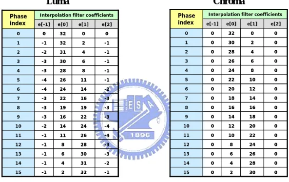
To decode this new type in enhancement layer, the block diagram of decoding process is described in Figure 17. The first step is to get the corresponding blocks in the lower resolution layer. After the reference blocks in the lower resolution layer are identified, these reconstructed samples are upsampled to the higher resolution layer. In the SVC design, the upsampling process for the luma samples consists of applying a separable four-tap poly-phase interpolation filter. The interpolation coefficient values for the filter are provided in Table 3. The chroma samples are also upsampled but with a different (simpler) interpolation filter which corresponds to bi-linear interpolation. The interpolation coefficients of this filter are also shown in Table 3.

The use of different interpolation filters for luma and chroma is motivated by complexity considerations. In prior standardized designs, the upsampling filter was only bi-linear for both luma and chroma, but resulting in significantly lower luma prediction quality. Therefore, the SVC standardizes different filters to luma and chroma samples.

(40)

Figure 17: Block diagram of Intra_BL decoding process.

Table 3: Interpolation coefficients for Luma and Chroma up-sampling.

Luma Chroma -1 11 26 -4 5 -2 14 24 -4 6 -3 16 22 -3 7 -3 19 19 -3 8 -3 22 16 -3 9 -4 24 14 -2 10 -4 26 11 -1 11 -3 28 8 -1 12 -1 32 2 -1 15 -2 31 4 -1 14 -3 30 6 -1 13 -1 8 28 -3 4 -1 6 30 -3 3 -1 4 31 -2 2 -1 2 32 -1 1 0 0 32 0 0 e[2] e[1] e[0] e[-1]

Interpolation filter coefficients

Phase index -1 11 26 -4 5 -2 14 24 -4 6 -3 16 22 -3 7 -3 19 19 -3 8 -3 22 16 -3 9 -4 24 14 -2 10 -4 26 11 -1 11 -3 28 8 -1 12 -1 32 2 -1 15 -2 31 4 -1 14 -3 30 6 -1 13 -1 8 28 -3 4 -1 6 30 -3 3 -1 4 31 -2 2 -1 2 32 -1 1 0 0 32 0 0 e[2] e[1] e[0] e[-1]

Phase index 0 10 22 0 5 0 12 20 0 6 0 14 18 0 7 0 16 16 0 8 0 18 14 0 9 0 20 12 0 10 0 22 10 0 11 0 24 8 0 12 0 30 2 0 15 0 28 4 0 14 0 26 6 0 13 0 8 24 0 4 0 6 26 0 3 0 4 28 0 2 0 2 30 0 1 0 0 32 0 0 e[2] e[1] e[0] e[-1]

Phase index

After upsampling, the SVC decoder also adds the residual difference information to refine the upsampled prediction as the same as in H.264. Finally, a deblocking filter that is similar to that of the ordinary H.264/AVC but with altered boundary strength calculations is applied to the decoded result.

It should be noticed that the up-sampling process in Figure 17 is consisted of two parts. One is basic interpolation and the other one is extended vertical interpolation. However, the extended vertical interpolation process is only applied to some combinations of picture type in base layer and enhancement layer, such as frame-MBAFF, MBAFF-frame, and field-frame

(41)

Chapter 3 Proposed Intra Prediction Engine with

Data Reuse in H.264/AVC HP

In Chapter 1 and Chapter 2, the intra decoding process based on profile, picture type, and prediction source in H.264 and SVC is introduced. Therefore, we propose a H.264/SVC intra prediction engine which can support high profile and each inter-layer prediction type in single layer decoding and multi-layer layer decoding of H.264 and SVC, respectively.

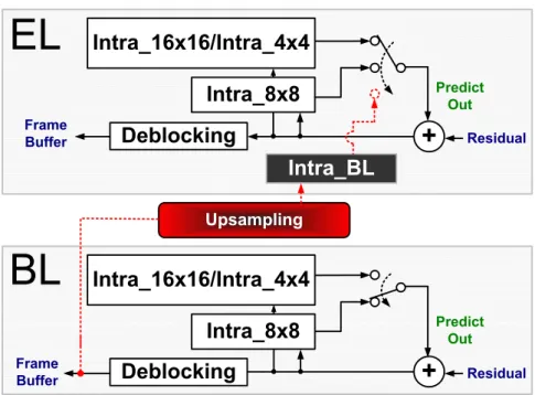
Figure 18: Block diagram of SVC intra prediction engine.

Figure 18 shows our proposed H.264/SVC intra prediction engine. The module “Basic Intra Prediction” is used to decode the traditional single layer intra prediction in H.264 or base layer intra prediction in SVC. The other module “Intra_BL Prediction” is designed to decode the new prediction type Intra_BL in enhancement layer of SVC.

(42)

described. Another design for SVC inter-layer intra prediction will be further described in Chapter 4. To alleviate the starved bandwidth of intra compensation in high-definition video, we reuse the neighboring pixels and optimize the buffer size and access latency. In particular, a dedicated pixel buffer reuses neighboring pixel for realizing MB-adaptive frame-field (MBAFF) decoding in intra compensation. Moreover, a base-mode predictor is explored to optimize the area efficiency for reference sample filtering process (RSFP) in intra 8x8 modes. The slightly increased gates and SRAMs overhead are 10% and 7.5% as compared to the intra prediction design with main profile. Simulation results show that the proposed data-reused intra prediction module requires 14K logic gates and 688 bits SRAM, and operates on 100MHz frequency for realizing 1080HD video playback at 30fps.

3.1 Overview

As we know, H.264/AVC consists of three profiles which are defined as a subset of technologies within a standard usually created for specific applications. Baseline and main profiles are intended as the applications for video conferencing/mobile and broadcast/storage, respectively. Considering the H.264-coded video in high profile, it targets the compression of high-quality and high-resolution video and becomes the mainstream of high-definition consumer products such as Blu-ray disc. However, high-profile video is more challenging in terms of implementation cost and access bandwidth since it involves extra coding engine, such as macroblock-adaptive frame field (MBAFF) coding and 8×8 intra coding, for achieving high performance compression.

In the MBAFF-coded pictures, they can be partitioned into 16x32 macroblock pairs, and both macroblocks in each macroblock-pair are coded in either frame or field mode. As compared to purely frame-coded pictures, MBAFF coding requires two times of neighboring pixels size and therefore increases implementation cost. To cope with aforementioned

(43)

problem, we propose neighboring buffer memory (include upper/left/corner) to reuse the overlapped neighboring pixels of an MB pair. Furthermore, we present memory hierarchy and pixel re-ordering process to optimize the overall memory size and external access efficiency. On the other hand, H.264 additionally adopts intra 8×8 coding tools for improving coding efficiency. It involves a reference sample filtering process (RSFP) before decoding a Luma

intra_8x8 block. These filtered pixels are used to generate predicted pixels of 8×8 blocks.

Hence, the additional processing latency and cost are required, and they may impact the overall performance for the real-time playback of high-definition video. In this chapter, we simplify the RSF process via a base-mode predictor and optimize the processing latency and buffer cost. Compared to the existing design [16] without supporting intra 8×8 coding, this design only introduces area overhead of 10% and 7.5% of gate counts and buffer SRAM.

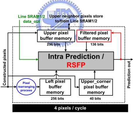
Figure 19: Block diagram of the proposed H.264 high-profile intra predictor.

Figure 19 shows the block diagram of the proposed H.264 high-profile intra compensation architecture. A pixel rearranging process, which is located on the bottom-left of Figure 19, is proposed to reduce the complexity of neighbor fetching when MBAFF coding is

(44)

enabled. The signal, Line SRAM1/2 data_out, is directly connected to the intra prediction block for replacing the last set of upper buffer memory. As for 8×8 intra coding, a dedicated pixel buffer memory is used to store the filtered neighboring pixels and reuse the overlapped pixel data. According to the relations between Luma intra_8x8 modes and numbers of filtered pixels which are needed in each mode, we minimize the number of stored pixels to 17 (i.e. 136 bits). The output of predicted pixel is interfaced to the filtered pixel buffer memory because RSFP is embedded in the intra prediction generator.

3.2 Memory Hierarchy

An architectural choice advocated for dealing with long past history of data is a memory hierarchy [18]. However, if the instantaneously used upper neighboring pixels are not in the neighboring information memory (i.e. a miss is occurring), the decoding process and pipeline schedule will be delayed and destroyed due to external SDRAM accessing. For more details, please refer [18]. In the intra prediction, it utilizes the neighboring pixels to create a reliable predictor, leading to dependency on a long past history of data. This dependency can be solved by storing upper rows of pixels for predicting current pixels but is a challenging issue in implementation cost and access bandwidth.

(45)

To optimize the introduced buffer cost and access efficiency, we use two internal Line SRAM1 and Line SRAM2 to store the Luma and Chroma upper line pixels, as illustrated in Figure 20. By the ping-pong mechanism, the upper neighboring pixels of current MB (or MB pair) are stored to one of them, and the other Line SRAM is used to store next MB of upper neighboring pixels. This memory hierarchy facilitates the internal Line SRAM size and the decoding pipeline schedule.

3.3 MBAFF Decoding with Data Reuse Sets

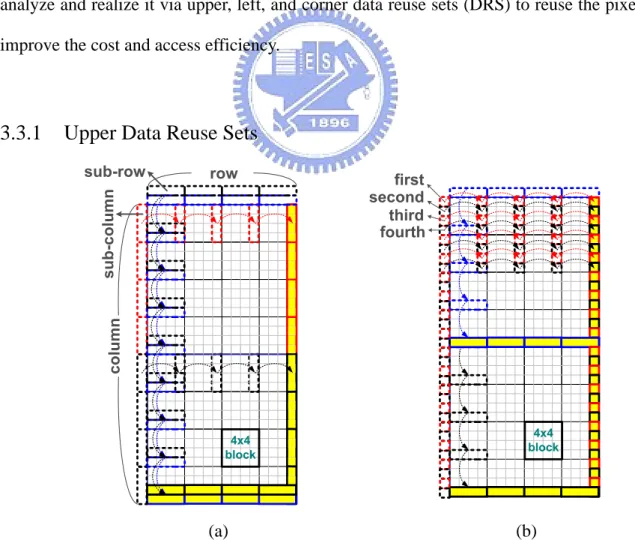
MBAFF is proposed to improve coding efficiency for interlaced video. However, it introduces longer dependency than conventional frame-coded picture. In this section, we analyze and realize it via upper, left, and corner data reuse sets (DRS) to reuse the pixels and improve the cost and access efficiency.

3.3.1 Upper Data Reuse Sets

(a) (b)

Figure 21: The updated direction of upper/left buffer memory in (a) frame and (b) field mode MB pair.

(46)

For decoding an MBAFF-coded video, upper buffer memory is used to store the constructed upper pixels of current MB pair. These upper buffers are updated with the completion of prediction process on every 4×4 block. For each updated sub-row(s), they can be reused by the underside 4×4 blocks. According to the different prediction modes of MB pair, the upper buffer will store data from different directions. If current MB pair is frame mode, it only needs to load one row of upper buffer (16 pixels) at first, and when a 4×4 block is decoded, updating the two sub-rows in two rows (8 pixels) of upper buffer from top to down at one time, as illustrated in Figure 21(a). Finally, the new pixels in two rows will be stored to Line SRAM in chorus when MB pair is decoded.

In Figure 21(b), a field-coded MB pair needs to load two rows of upper buffer (32 pixels), two times of frame-coded MB pairs. Then, only one sub-row of upper buffer memory will be updated when a 4×4 block is decoded. Finally, the new pixels in one row of upper buffer are stored back to Line SRAM when the top MB is decoded and another row of upper buffer are stored back to Line SRAM when the bottom MB is decoded. However, considering the fifth 4×4 block, it still needs a sub-row of upper buffer to predict, as shown in Figure 22. In order to reduce the upper buffer memory size, the Line SRAM data_out is directly used. The only penalty to this scheme is that the Line SRAM data_out must hold the value until fifth 4×4 block is decoded.

(47)

3.3.2 Left Data Reuse Sets

The updated direction of the left buffer is similar to that of the upper one. The direction ranges from left to right. When the left buffer is located on the right hand side of MB pair, the next MB pair can reuse these new pixels for the following prediction procedures. However, when the modes of current and previous MB pairs are different, the left neighbors of a 4x4 block will become complicated. To reduce computational complexity of this intra predictor, pixel rearranging process is exploited. If current MB pair is frame mode, each sub-column of left buffer will be updated when each 4x4 block is decoded, as shown in Figure 22(a). On the other hand, if current MB pair is field mode, first and third buffers in each sub-column of left buffer will be updated when each 4×4 block is decoded in the top MB, as shown in Figure 22(b). Second and fourth buffers in each sub-column of left buffer will be updated when each 4×4 block is decoded in bottom MB. Hence, we only need to consider what the mode current MB pair is, instead of handling four coding modes for the combination of current and previous MB pairs, and therefore the complexity can be reduced.

3.3.3 Corner Data Reuse Sets

Using corner buffer memory can efficiently reuse the upper left neighboring pixels. We change the positions of corner buffer from left [16] to top. Therefore, the total corner buffer size can be reduced by 38% (i.e. 64bits  40bits, because the MB number in horizontal is less than that of vertical MB pair). In particular, Figure 23 shows the updating directions of corner buffer. However, because the upper neighboring pixels will be either the last row or the row prior to the last row in upper MB pair, hence the first corner of current MB pair has two processing states: reuse and reload. The first corner is reused when 1) the mode of current MB pair is identical to that of previous (left) MB pair or 2) before decoding the bottom MB of frame-coded MB pair. On the other hand, the first corner is reloaded when 1) the current MB

(48)

pair has the different modes as previous (left) MB pair or 2) before decoding the bottom MB of field-coded MB pair.

Figure 23: The updated direction of corner pixel buffers.

In summary, using neighboring buffer memory and their different directions of updates according to different modes of MB pair can reuse the neighboring pixels and improve the

(49)

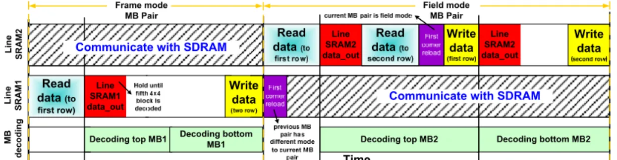
access efficiency. The associated pipeline structure of MBAFF decoding is shown in Figure 24. We can see that during a MB pair decoding process, the interaction between buffers and Line SRAM can be completed easily and efficiently, and the communication between another Line SRAM and external SDRAM can be done at the same time. It should be noticed that Line SRAM1/2 data_out must be held until the fifth 4x4 block is decoded.

Figure 24: The pipeline scheme of MBAFF decoding.

3.4 Intra 8x8 Decoding with Modified Base-Mode Intra

Predictor

Luma intra_8x8 is an additional intra block type supported in H.264 high profile. Before decoding an intra_8x8 block, there is an extra process that is different from intra_4x4 and

intra_16x16, which called reference sample filtering process (RSFP). Original pixels will be

filtered first, and then using these filtered pixels to predict subsequent 8×8 blocks.

3.4.1 Filtered Neighboring Buffer Analyze

For an intra_4x4 and intra_8x8 block, 13 neighbors and 25 filtered neighbors are needed, respectively. However, according to the Luma intra_8x8 modes, the maximum number of filtered neighbors is 17, as illustrated in Table 4. Hence, only 17 (i.e. 136 bits) filtered pixels of a 8x8 block need to be stored in our filtered pixel buffer memory instead of storing all of

(50)

the 25 filtered neighbors.

Table 4: Number of filtered pixels actually needed in intra 8x8 modes.

Prediction Modes of Intra_8x8 # of filtered neighbors

0 (Vertical) 8 1 (Horizontal) 8

2 (DC) 0,8,16

3 (Diagonal down left) 16 4 (Diagonal down right) 17 5 (Vertical right) 17 6 (Horizontal down) 17 7 (Vertical left) 16 8 (Horizontal up) 8

3.4.2 Reference Sample Filter Process (RSFP)

In the intra_4x4 process, the prediction formula of each mode except DC mode has the same form: prediction_out = (A+B+C+D+2) >> 2. For a four-parallel intra pixel generator, a suitable architecture design is proposed in [14], as shown in Figure 25.

Figure 25: Intra predictor in [14].

However, if we analyze the relationship between four output pixels in each mode, some adders can be eliminated due to the shared items, so that the hardware architecture can be reduced [19], as described in Figure 26. This shared based intra predictor can predict almost

(51)

every intra_4x4 mode in one cycle. But there still exist exceptions, such as vertical-right. For example, in the vertical-right prediction mode, there is no shared item between prediction pixels m and n, as illustrated in Figure 27. Therefore, the modified intra predictor is proposed. Compared with the share-based [14]-[16][19] intra prediction generator, the proposed base-mode intra predictor not only reduces area cost (due to elimination of four adders) but also guarantees that four predicted pixels will be generated in one cycle of each intra_4x4 modes. I+Q+Q+A J+I+I+Q K+J+J+I L+K+K+J p o n m Q+A+A+B I+Q+Q+A J+I+I+Q K+J+J+I L k j i A+B+B+C Q+A+A+B I+Q+Q+A J+I+I+Q H g f e B+C+C+D A+B+B+C Q+A+A+B I+Q+Q+A d c b a I+Q+Q+A J+I+I+Q K+J+J+I L+K+K+J p o n m Q+A+A+B I+Q+Q+A J+I+I+Q K+J+J+I L k j i A+B+B+C Q+A+A+B I+Q+Q+A J+I+I+Q H g f e B+C+C+D A+B+B+C Q+A+A+B I+Q+Q+A d c b a

Figure 26: Intra predictor in [19].

2B+C+A 2A+M+B 2M+I+A 2J+K+I P o n m 2B+C+C 2A+M+B 2M+A+A 2I+J+M L k j i 2C+B+D 2B+A+C 2A+M+B 2M+I+A H g f e 2C+D+D 2B+C+C 2A+B+B 2M+A+A d c b a 2B+C+A 2A+M+B 2M+I+A 2J+K+I P o n m 2B+C+C 2A+M+B 2M+A+A 2I+J+M L k j i 2C+B+D 2B+A+C 2A+M+B 2M+I+A H g f e 2C+D+D 2B+C+C 2A+B+B 2M+A+A d c b a No shared item

Figure 27: Modified base-mode intra predictor.

In particular, we use this base mode predictor to generate the four predicted pixels in one cycle. In the RSFP, the form of formula is identical to that in intra_4x4, and also can be rewritten to the same form filtered_out = (A+2B+C+2) >> 2. Hence, we can share the hardware resource to generate filtered pixels, as shown in Figure 28. Notice that an additional process, neighbor distribution, is needed to apply in intra_8x8 process because we only store 17 filtered pixels instead of 25.

應用於SVC視訊編碼標準之空間可適性內幀解碼器設計

國立交通大學

電子工程學系 電子研究所碩士班

碩 士 論 文

應用於 SVC 視訊編碼標準之空間可適性內幀解碼器設計

Design of An Intra Predictor with Spatial Scalability

for Scalable Video Decoding

學生 ： 賴昱帆

指導教授 ： 李鎮宜 教授

應用於 SVC 視訊編碼標準之空間可適性內幀解碼器設計

Design of An Intra Predictor with Spatial Scalability

for Scalable Video Decoding

研 究 生：賴昱帆 Student：Yu-Fan Lai

指導教授：李鎮宜 博士 Advisor：Dr. Chen-Yi Lee

國 立 交 通 大 學

電子工程學系 電子研究所碩士班

碩 士 論 文

應用於 SVC 視訊編碼標準之空間可適性內幀解碼器設計

學生：賴昱帆 指導教授：李鎮宜 教授

國立交通大學

電子工程學系 電子研究所碩士班

摘要

Design of An Intra Predictor with Spatial Scalability for

Scalable Video Decoding

Student : Yu-Fan Lai Advisor : Dr. Chen-Yi Lee

Department of Electronics Engineering

Institute of Electronics

National Chiao Tung University

ABSTRACT

誌

謝

Contents

List of Figures

List of Tables

Chapter 1

Introduction

1.1 Motivation

1.2 Thesis Organization

Chapter 2

Overview the Intra Prediction in

H.264/AVC and Scalable Video Coding

2.1 H.264/AVC Standard Overview

2.1.1 Profiles and Levels

2.1.2 Encoder/Decoder Block Diagram

2.1.4 Macroblock-Adaptive Frame-Field Intra Decoding

2.1.4.1 Types of Video Source Formats

2.1.4.2 Intra Block Neighboring Information in MBAFF

2.1.5 Intra_8x8 Prediction Mode Decoding

2.2 SVC Extension of H.264/AVC Standard Overview

2.2.1 Profiles and Levels

2.2.2 Encoder/Decoder Block Diagram

2.2.3 Special Features in SVC

2.2.3.1 Spatial Scalability

2.2.4 Inter-Layer Intra-Prediction

2.2.4.1 Intra_BL Decoding Processes

Chapter 3

Proposed Intra Prediction Engine with

Data Reuse in H.264/AVC HP

3.1 Overview

3.2 Memory Hierarchy

3.3 MBAFF Decoding with Data Reuse Sets

3.3.1 Upper Data Reuse Sets

3.3.2 Left Data Reuse Sets

3.3.3 Corner Data Reuse Sets

3.4 Intra 8x8 Decoding with Modified Base-Mode Intra

Predictor

3.4.1 Filtered Neighboring Buffer Analyze

3.4.2 Reference Sample Filter Process (RSFP)

電子工程學系電子研究所碩士班

碩士論文

學生：賴昱帆

指導教授：李鎮宜教授

研究生：賴昱帆 Student：Yu-Fan Lai

指導教授：李鎮宜博士 Advisor：Dr. Chen-Yi Lee

國立交通大學

電子工程學系電子研究所碩士班

碩士論文

學生：賴昱帆指導教授：李鎮宜教授

電子工程學系電子研究所碩士班