應用不變量澤爾尼克矩描述元進行影像之表示、比對及辨識

(1)

國

立

交

通

大

學

資訊學院

資訊科學與工程研究所

博

士

論

文

應用不變量澤爾尼克矩描述元

進行影像之表示、比對及辨識

Image Representation, Matching, and Recognition

Using Invariant Zernike Moment Descriptors

研究生：孫樹國

指導教授：陳稔教授

(2)

應用不變量區域描述元進行影像之表示、比對及辨識

Image Representation, Matching, and Recognition

Using Invariant Zernike Moment Descriptors

研究生：孫樹國 Student：Shu-Kuo Sun

指導教授：陳稔 Advisor：Zen Chen

國立交通大學

資訊學院

資訊科學與工程研究所

博士論文

A Dissertation

Submitted to Institute of Computer Science and Engineering College of Computer Science

National Chiao Tung University in Partial Fulfillment of the Requirements

for the Degree of Doctor of Philosophy

in

Computer Science July 2009

Hsinchu, Taiwan, Republic of China

(3)

進行影像之表示、比對及辨識

研究生：孫樹國指導教授：陳稔博士

國立交通大學

資訊學院

資訊科學與工程研究所

摘要

本論文在探討三維電腦視覺中，利用二張或更多張不同視度或不同光照條件下所拍攝的景物影像來進行景物分析、辨識及套合等研究，所需克服影像間存在之幾何轉換 (旋轉、尺度變化、平移及幾何變形)、影像亮度轉換 (影像模糊、照度改變、雜訊、影像壓縮等)、部分遮蔽以及影像套合計算效率等問題。首先，我們提出一個基於澤爾尼克矩相位資訊為主的不變量區域描述元，同時包含精確估算二個特徵區域間旋轉角度的方法來解決旋轉方位對齊的問題，以及一個可以達到高可靠度的比對函式。整體而言，在上述不同的幾何及影像亮度轉換下，這個新的澤爾尼克矩相位描述元較諸目前五個主要方法具有更高的區辨能力，論文中亦包含定性及定量分析來說明這些描述元效能差異的原因。其次，我們將這個區域描述元延伸到行動裝置服務之商標符號辨識上，它可使用於

(4)

企業識別、公司網頁存取、交通安全號誌辨認及安全檢查等相關應用上，在此主要的挑戰是行動裝置拍攝影像時所無法避免的幾何及影像亮度轉換，我們提出二種相似度量測方法分別用於分類及檢索上，實驗顯示我們提出的方法較之既有的三個主要方法具有更好的效能。最後，我們提出一個不同於傳統之影像套合方法，更有效率的達到不同視點影像套合所需之一對一特徵點對應，此方法是基於事先分析參考影像以獲取重要的資訊來引導影像套合程序之進行。首先，在離線階段先針對參考影像中的特徵點根據下述五個規劃策略來事先建立挑選順序之資料庫: (1)特徵點對影像變形之不變量、(2)對影像雜訊之抵抗力、(3)描述元之區辨能力、(4)模型估算之有效性及(5)影像部份重疊之處理能力。因此，當我們獲得感測影像進行影像套合時，即可更有效率的建立這二張影像間之特徵點一對一對應關係，來估算這二張影像的轉換模型。

(5)

Image Representation, Matching, and Recognition

Using Invariant Zernike Moments Descriptors

Student：Shu-Kuo Sun Advisor：Dr. Zen Chen

Institute of Computer Science and Engineering

College of Computer Science

National Chiao Tung University

ABSTRACT

In 3D computer vision a scene in the real world is represented by multiple views imaged under different viewpoints and illumination conditions. The spatial and temporal relationships across these views are important to scene analysis and understanding. To derive these relationships the global and local features of the objects (foreground and background) in the scene are the clues. The local features related to the local object surface patches or regions are more robust to viewpoint change than the global features. In addition, the invariance under the photometric transformations such as blur, illumination, scale, noise, JPEG compression is also receiving great attention.

In this dissertation subjects related to the local image representation, matching, and recognition under the above image variations are addressed. First, a new distinctive image descriptor to represent the normalized regions extracted by an affine region detector is proposed which primarily comprises the Zernike moment (ZM) phase information. An accurate and robust estimation of a possible rotation angle between a pair of normalized

(6)

regions is then described, which will be used to measure the similarity between two matching regions. The discriminative power of the new ZM phase descriptor is compared with five major existing region descriptors based on the precision-recall criterion. The experimental results involving more than 15 million region pairs indicate the proposed ZM phase descriptor has, overall speaking, the best performance under the common photometric and geometric transformations. Both quantitative and qualitative analyses on the descriptor performances are given to account for the performance discrepancy.

Second, the proposed ZM phase descriptor is further extended to present a new recognition method of logos imaged by mobile phone cameras. The logo recognition can be incorporated with mobile phone services for use in enterprise identification, corporate website access, traffic sign reading, security check, content awareness, and the related applications. The main challenge to applying the logo recognition for mobile phone applications is the inevitable photometric and geometric transformations. The proposed ZM phase recognition method is associated with two similarity measures. The logo classification and retrieval experimental results show that the proposed ZM phase method has the best performance under the typical photometric and geometric transformations, compared with other three major existing methods.

Finally, as for the one-to-one feature matching correspondences in view registration, we propose an efficient registration method different from the traditional methods. We take advantage of preprocessing of the reference image offline to gather the important statistics for guiding image registration. That is, we introduce five planning strategies to sort the feature points in the reference image based on the concepts of (1) feature invariance to image deformation, (2) image noise resistance, (3) distinctive description power, (4) model estimation effectiveness, and (5) partial image overlapping handling capability. Thus, a

(7)

reference matching database is constructed offline using the above five planning strategies. Then, an online registration process is presented to estimate the transformation model to overlay the reference image over an incoming sensed image. In this way, better registration efficiency can be achieved.

(8)

ACKNOWLEDGEMENTS

I wish to express my sincere appreciation to my advisor, Dr. Zen Chen, for his kind patience, constant encouragement, helpful guidance, inspiration throughout, and the invaluable training the course of this dissertation. In these years, he has stimulated the research work and teaches me how to learn and how to think interpedently. Especially, he encourages me to challenge what we are used to be. I also express my sincere gratitude to the members of my thesis committee, Professor Chuang and Professor Wang, for their valuable suggestions and comments.

Finally, I am so grateful to my wife, my parents, and my children for their love, support, and tolerance during the dissertation study. This dissertation is dedicated to them.

(9)

LIST OF FIGURES

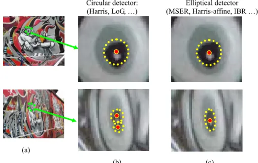
Fig. 1.1: Two images taken from different view-points and the detected regions by circular detector and Elliptical detector. ...2 Fig. 3.1: Plots of the real part and imaginary part of Vnm (ρ, θ) for a fixed n...18 Fig. 3.2: The reference coin image and its rotated variant, inverted variant and mirrored variant with the diagrams of the ZM phase differences and the ZM magnitude components...23 Fig. 3.3: Representative test image pairs taken from the textured and structured scenes

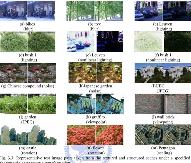
under a specified photometric or geometric transformation...27 Fig. 3.4: The PR curve generation process with a varying distance threshold...30 Fig. 3.5: Evaluation for different overlap errors for structured scene using the detected

Hessian-affine regions and MSER regions under viewpoint change. ...32 Fig. 3.6: Evaluation for different overlap errors for textured scene using the detected

Hessian-affine regions and MSER regions under viewpoint change. ...33 Fig. 3.7: The examples of the detected region pairs with different overlap errors ranging

from 0.1 to 0.6. ...34 Fig. 3.8: The PR curves for the structured bike scene and textured tree scene with minor

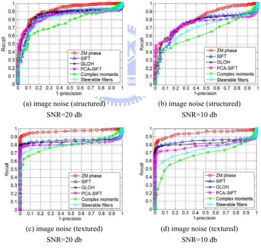
blur and severe blur.. ...37 Fig. 3.9: The correct matches and false matches obtained by the descriptors...38 Fig. 3.10: The PR curves for the Leuven structured scene and the bush 1 textured scene

with affine lighting change, underexposure non-linear lighting change, and overexposure non-linear lighting change. ...39 Fig. 3.11: The PR curves for the Chinese compound structured scene and the Japanese

(12)

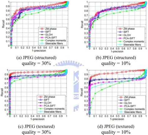
Fig. 3.12: The PR curves for the structured UBC scene and the textured garden scene under

JPEG compression with quality = 30% and 10%...41

Fig. 3.13: The PR curves under geometric transformation...43

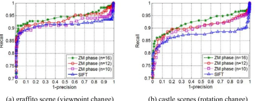
Fig. 3.14: The PR curves for ZM phase with the maximum order N = 10, 12 and 16, together with the associated PR curves of SIFT for two structured scenes under two different attacks. ...44

Fig. 3.15: A performance comparison of ZM phase and SIFT under non-linear lighting change...47

Fig. 3.16: A performance comparison of ZM phase and SIFT under JPEG compression....48

Fig. 3.17: A performance comparison of ZM phase and SIFT under Viewpoint change. ....49

Fig. 3.18: A performance comparison of ZM phase and SIFT under scaling change. ...50

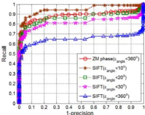
Fig. 3.19: The PR curves for tree textured scene under image blur with the removal of regions with a rotation angle error not exceeding a specified level ...53

Fig. 4.1: A scenario of the mobile applications for logo recognition. ...57

Fig. 4.2: Three logo images taken from different viewpoints and their normalized images. ...60

Fig. 4.3: The set of similar logos. ...63

Fig. 4.4: The classification results for three logo queries...64

Fig. 4.5: Some of 300 logos used in the experiment. ...65

Fig. 4.6: The PR curves for retrieval performance evaluations under different kinds of specified transformations...66

Fig. 4.7: Some of 100 traffic signs used in the experiment. ...67

Fig. 4.8: The traffic sign retrieval results.. ...68

Fig. 4.9: A performance analysis on the ZM phase, IZMD, EHD and Ring projection methods under image blur. ...71

(13)

Fig. 5.1: The architecture of the proposed view registration process...73 Fig. 5.2: The point sets and the dominant orientation sets in the reference image and the

sensed image...78 Fig. 5.3: The triangle formed by the two feature points and their dominant orientations....83 Fig. 5.4: The reference image and the synthetic sensed image for view registration...88 Fig. 5.5: The partial overlapping between the image boundaries of the reference and three transformed sensed images, and the view registration results...89 Fig. 5.6: The effect of image noise on the ranking of reference feature points according to the product of normalized energy and orientation factor...91 Fig. 5.7: Two real building images that are partially overlapped, and the final registration

result.. ...92 Fig. 5.8: Three synthetic landscape images used for view registration, and the final

(14)

LIST OF TABLES

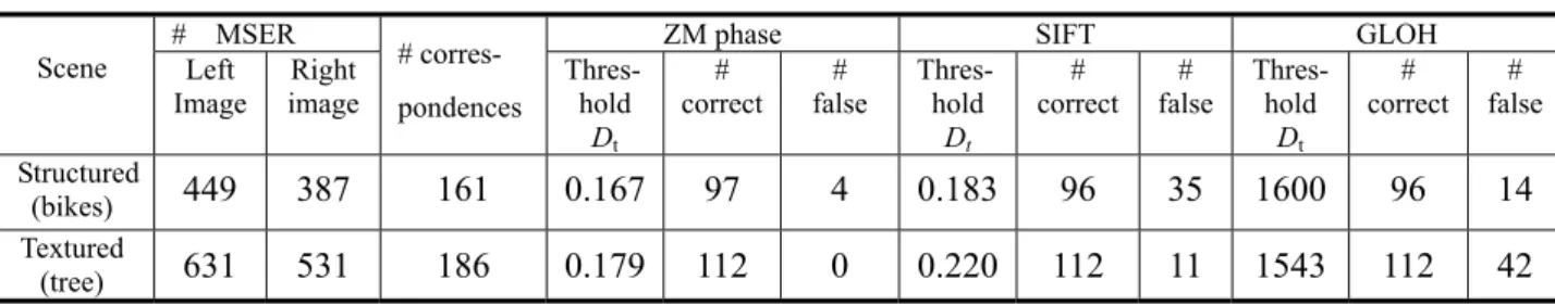
Table 2.1 A paradigm of view transformation estimation methods...14 Table 3.1 List of ZMs sorted by nand m in sequence for the case where (n m, ) = (12, 12)19 Table 3.2 The typical feature vector dimensions of the six descriptors...27 Table 3.3 The matching statistics for the bike structured scene and tree textured scene, all with

t

O= 0.3 and recall = 0.6. ...38 Table 3.4 The rotation angle estimation errors for all corresponing region pairs specified

byO_t= 0.3...52

Table 5.1 The construction of SPP_i from the four sub-regions. ...85 Table 5.2 The transformation parameters produced in the three iterations ...90 Table 5.3 The statistic of the online registration process for registering two building images 93 Table 5.4 Registration efficiency comparison with and without the off-line planning strategies

(15)

Introduction

1.1 Problems Statement

In 3D computer vision a scene in the real world is represented by multiple views when imaged under different viewpoints and illumination conditions. The spatial and temporal relationships across these views are important to scene analysis and understanding. To derive these relationships the global and local features of the objects (foreground and background) in the scene are the clues. Global features such as Fourier descriptors describe the scene information as the scene is seen in the 2D image as a whole. The global features are suitable for deriving the relationships when the objects of concern have the same appearances in the different views. Generally, the objects have different surface appearances under different viewpoints, especially when the background and foreground objects are partially overlapped, so the global image features are often not invariant to the viewpoint. On the other hand, the local features related to the local object surface patches or regions are more robust to viewpoint change. In addition, the invariance under the photometric transformations such as blur, illumination, scale, noise, JPEG compression is also receiving great attention. The invariant local features are crucial to most image understanding and computer vision applications including image matching, camera calibration, texture classification, and image retrieval, etc. [1]-[5].

The processing of local features involves three tasks: feature detection, feature description, and feature matching. The local features belong to an interest point (keypoint) or

(16)

an interest region. Since a single image point carries little information, an interest point must be associated with its surrounding image patch. From this image patch a second moment matrix of image intensities reveals the characteristic structure of the local image region. The keypoint detectors such as Harris corner detector [6] and the SIFT detector [7], which is based on the difference of Gaussians (DOG), utilize a circular window to search for a possible location of a keypoint. However, the image content in the circular window is not robust to affine deformations. Furthermore, the feature points may not be reliable and may not appear simultaneously across the view-point change, as illustrated in Fig. 1.1(b). Recently, a number of local feature detectors using a local elliptical window have been investigated. The affine covariant regions offer a unique solution to viewpoint change, as illustrated in Fig. 1.1(c). Matas et al. [5] presented a maximally stable extremal region (MSER) detector. Tuytelaars and Van Gool [8] developed an edge-based region (EBR) detector as well as an image-based (IBR) region detector. Mikolajczyk and Schmid [9] proposed Harris-Affine and Hessian-Affine detectors. The performances of the existing region detectors were evaluated in [11] in which the MSER detector and the Hessian-Affine detector were the two best.

Fig. 1.1: (a) Two images taken from different viewpoints. (b) The detected regions by a circular detector. Circular detector:

(Harris, LoG, …) (MSER, Harris-affine, IBR …)Elliptical detector

(b) (c)

(17)

In the descriptor construction, the detected ellipse-shaped region is first normalized to a circular patch of a fixed size. The normalized circular patch can be shown to be affine invariant up to a rotational ambiguity [10, 33]. A good feature descriptor to describe the normalized circular patch should be invariant (unchanged under the spatial transformation), distinctive (unique in feature description), stable (robust to image deformation) and independent (uncorrelated relation between feature descriptors).

After the region descriptor is determined, a matching function is defined to measure the similarity between regions extracted from different images of the same scene. The merits of various region detectors, coupled with their own region descriptors, are often judged based on the ROC (receiver operating characteristic) curve or the PR (precision-recall) curve.

1.2 Sketch of the Work

In this dissertation, three themes related to the image representation, matching, recognition, and view registration under the aforementioned geometric and photometric transformations are addressed.

In the first theme, the representation and matching power of region descriptors are to be evaluated. A common set of elliptical interest regions is used to evaluate the performance. The elliptical regions are further normalized to a circular one with a fixed size (typically, 41 by 41 pixels). Here a new distinctive image descriptor to represent the normalized region is proposed which primarily comprises the Zernike moment (ZM) phase information. An accurate and robust estimation of the rotation angle between a pair of normalized regions is then described, which will be used to measure the similarity between two matching regions. The discriminative power of the new ZM phase descriptor is compared with five other major

(18)

region descriptors (SIFT, GLOH, PCA-SIFT, complex moments, and steerable filters) based on the precision-recall criterion. To match the region pairs, a new distance measure based on the ZM phase information is defined. For performance evaluation, important system parameters must be taken into consideration, which include (1) region scene types, (2) region descriptor types, (3) region detector types, (4) region overlap error, and (5) transformation types. From the experimental results involving more than 15 million region pairs the proposed ZM phase has the best overall performance under the aforementioned photometric and geometric transformations. Both quantitative and qualitative analyses on the descriptor performances are given to account for the performance discrepancy.

In the second theme, the proposed ZM phase descriptor is further extended to present a new recognition method of logos imaged by mobile phone cameras. The logo recognition can be incorporated with mobile phone services for use in enterprise identification, corporate website access, traffic sign reading, security check, content awareness, and the related applications. The main challenge to applying the logo recognition for mobile phone applications is the inevitable photometric and geometric transformations encountered when using a handheld mobile phone camera operating at a varying viewpoint during the daytime or the nighttime. The discriminative power of the new logo recognition method is compared with three major existing methods. The experimental results indicate the proposed ZM phase method has the best performance in terms of the precision and recall criterion under the above inevitable imaging variations.

In the third theme, we propose an efficient registration method for the one-to-one feature matching correspondences in view registration. We take advantage of preprocessing of the reference image offline to gather the important statistics for guiding image registration. That is, we introduce five planning strategies to sort the feature points in the reference image based

(19)

on the concepts of (1) feature invariance to image deformation, (2) image noise resistance, (3) distinctive description power, (4) model estimation effectiveness, and (5) partial image overlapping handling capability. The invariant feature points are extracted from the reference image and a reference matching database is constructed offline using the above five planning strategies. Then, an online registration process is presented to estimate the transformation model to overlay the reference image over an incoming sensed image. In this way better registration efficiency can be achieved.

1.3 Contribution of the Work

The main contributions of this dissertation can be summarized as follows:

(1) To design a new region descriptor and a new matching function based mainly on Zernike moment (ZM) phase information and show the ZM phase information is more distinctive than the ZM magnitude information in terms of image representation and matching.

(2) To propose an accurate estimation of the rotation angle between a region pair to be matched.

(3) To show the proposed ZM phase descriptor has the better overall performance than the five other major descriptors under common geometric and photometric transformations.

(4) To extend the ZM phase descriptor to design a new distinctive logo feature vector and two associated similarity measures for logo recognition, and to show the proposed ZM phase logo feature vector has better recognition and retrieval performance than other three existing methods.

(20)

(5) To develop a new view registration method that take advantage of preprocessing of the reference image offline to gather the important statistics for image registration, and achieves better view registration time complexity than other existing methods.

1.4 Dissertation Organization

The rest of this dissertation is organized as follows. Chapter 2 reviews existing literature on local region descriptors, methods for logo recognition, as well as methods for image registration. Chapter 3 presents our Zernike Moment phase based descriptor for local image representation and matching. Chapter 4 extends our Zernike Moment phase based descriptor to logo recognition. Chapter 5 presents five offline planning strategies and an online registration process for high-efficiency perspective view registration. Finally, Chapter 6 closes the dissertation with a summary of our work and a discussion on possible extensions and future research directions.

(21)

Previous Work

2.1 Region detectors and descriptors

A region descriptor is needed to derive the region features for region representation and matching after the regions of interest are detected. Here a brief introduction of five major classes of the existing descriptors is briefly given to explore their strengths and weakness in order to compare them with the proposed ZM phase based descriptor. An excellent review on the existing descriptors can be found in [12]-[13].

(1) Filter-based Descriptors:

This class of descriptors includes steerable filters [14] and Gabor filters [15]. The steerable filter descriptor uses quadrature pairs of derivatives of Gaussian and their Hilbert transforms to synthesize any filter of a given frequency with arbitrary phase. On the other hand, the Gabor transform uses a number of Gabor filters tuned to various frequencies and orientations to represent the image patterns. Both the steerable filter and the Gabor filter descriptors need to seek a dominant orientation for image rotation alignment. If the reference and transformed descriptor feature vectors are not aligned well, their matching score will be poor. Besides, these descriptors are not totally orthogonal and their feature vector dimensions are generally low, so their discriminative powers are limited.

(22)

(2) Moment-based descriptors:

The first class of moment-based descriptor is the geometric (or regular) moments. The (p+q) order moment of an intensity or gradient image f(x,y) is defined as follows

( , ), , 0, 1, 2, ...

p q

pq

x y

m =

∑∑

x y f x y p q=

Based on the geometric moments, a set of moment invariants can be derived from the nonlinear combinations of geometric moments to achieve affine invariance [16], [32]. The main problem with the geometric moments is that it is difficult to derive a sufficient number of invariants to describe complex shapes. Moreover, the higher-order moments are more sensitive to image noise than the lower-order moments. Therefore, the geometric moment invariants are usually suitable only for describing simple images [17].

The second moment class is the complex moments of the form

( , ) ( ) (m ) (n )

mn

x y

K x y =

∑∑

x iy+ x iy f x, y− where f(x, y) is an image intensity function [18], [19]. Any rotation of the image changes the phases of the complex moments, but not the magnitudes. That is, the magnitudes of the filter responses are rotational invariant. There are 16 filters, defined by m + n ≤ 6 and n ≤ m, available for image patch description. This low dimensional rotational invariant descriptor generally has a poor discriminative performance [12].

(3) Distribution-based descriptors:

This class of descriptors includes SIFT [7], GLOH [12], PCA-SIFT [22], spin image and RIFT descriptors [3]. They use the distributions of the image content to represent the features of the image region.

(23)

The SIFT descriptor is represented by a 3D histogram of gradient locations and orientations. The histogram of the gradient orientations is quantized in 8 bins and the region is partitioned into a 4×4 location grid, resulting in a feature vector of dimension 128. Although the gradient histogram provides stability against deformations of the image pattern, the grid partition of the measurement region has the boundary effect problem. Gaussian smoothing and tri-linear interpolation can be called to alleviate this problem. More importantly, SIFT requires an accurate dominant (gradient) orientation for image rotation alignment.

The PCA-SIFT descriptor is a dimension-reduced version of SIFT (dimension reduced from 3042 to 36 or lower) based on an eigenspace obtained by applying PCA to a collection of 21,000 image patches. On the other hand, the GLOH descriptor is also an extension of the SIFT descriptor. Instead of sampling gradient orientations in a rectangular grid, GLOH is defined in a log-polar location grid with 17 location bins. These location bins, together with 16 gradient orientation bins, form a feature vector of dimension 272. With PCA the feature dimension is reduced to 128 based on a training data set of 47,000 image patches.

The SIFT and its variants depend on a dominant orientation of the normalized patch to achieve the rotation invariance. However, according to the experience of Lazebnik et al. reported in [3], the dominant orientation estimation tends to be unreliable, especially for normalized Laplacian regions in which strong edges at the center are often not available. (4) Derivative-based descriptors:

This type of descriptors uses local derivatives, called “local jets”, to construct the differential invariants, which are rotationally invariant [23]. Schmid and Mohr [2] derive a set of differential invariants in terms of polynomials of local derivatives up to the third order for image retrieval. The derivative-based descriptors face with some problems: (a) the dimension

(24)

of the rotationally invariant differential invariants is generally low [12], and (b) the differential invariants are often sensitive to image blur or image noise if smoothing operation is not used beforehand. (The steerable filters can be also classified as a derivative-based descriptor.)

(5) Others:

Besides the above basic descriptor types, there are other extended descriptors including (i) color-based descriptors [21] which utilizes the color information for feature representation, (ii) textons [3], which are based on the responses of a texture image to a filter bank, can categorize the large-scaled texture images. In this paper, only the basic descriptors of the first four classes are concerned.

2.2 Logo Recognition

A logo is a graphic entity containing colors, shapes, textures, and perhaps text as well, organized in some spatial layout format. There are four major classes of the existing feature used for logo recognition:

(1) Color features:

Color feature are often easily obtained from the logo image. The color histogram [54] is probably one of the most popular gross representations of the foreground object in which the precise spatial information is lost, so an exact matching is generally impossible. Since a logo may be designed with a few setting of color combinations, color will be ignored as far as the unique identity of a logo (represented as an intrinsic graphic pattern) is concerned.

(25)

(2) Text features:

The text in the logo is often modified to add to its aesthetic appealing, its segmentation for the OCR processing may not be easy and also unnecessary for logo identification. The whole text can be viewed as part of the logo and handled with others by a general shape analyzer.

(3) Texture features:

Similarly, if a logo contains texture patterns, the texture patterns can be treated as a graphic pattern and, again, handled with other parts together. In the end, a logo representation is boiled down to an integrated shape pattern or a set of sub-logo shape patterns. Hence, shape analysis of the logo is the main concern here.

(4) Shape features:

Different methods using different shape features for logo classification have been proposed in the literature. Edge histogram descriptor (EHD) [58] is an MPEG-7 texture descriptor that captures the spatial distribution of edges. EHD is represented by a histogram of the gradient orientations which is quantized in 5 bins and the region is partitioned into a 4×4 location grid, resulting in a feature vector of dimension 80. Although the gradient histogram provides stability against mild deformations of the image pattern, the grid partition of the support region will lead to the non-smooth boundary feature values, i.e., the so-called boundary effect problem.

Recently, some researchers using Gabor transform and wavelet transform for pattern recognition [55]-[56]. However, the set of Gabor filters is not orthogonal, and thus reduce its discriminative power. On the other hand, the wavelet transform has the advantages of multiple

(26)

resolutions and reconstructability, but it is not rotational invariant (so is the Gabor transform). Therefore, both transforms need to solve the rotation problem first based on some orientation information.

To achieve rotation invariant, an alternative method using a ring projection structure is suggested in which the absolute sums of the sub-band coefficients (LH, HL and HH) of wavelet transform are accumulated within a specific number of rings [59]. However, the ring projection will lose the spatial information in the radial direction. As a consequence, a logo and its mirror version have the same ring projection profiles, and, therefore, become indistinguishable. More impotently, most of the above methods cannot work properly under photometric and geometric image transformations, as shall be seen.

2.3 View Registration

View registration is a process of overlaying images of the same scene taken at different imaging conditions [60-64]. View registration applications include satellite image registration [65, 66, 82, 83], medical view registration [61, 62], object recognition [69-70], motion tracking [71-73], image mosaic [74], automatic cartography [75], fundamental matrix estimation [76], and perspective reconstruction [74, 75]. Good survey on view registration can be found in [60-64].

Due to the variations in viewpoint, illumination and the sensor noise, the feature points may not be reliable and may not appear simultaneously across the multiple views. Therefore, the point correspondence validation is not a trivial task. One may skip the point correspondence matching and estimates the transformation model directly using an

(27)

appropriate number of feature point pairs. Traditionally, there are three major ways for the direct registration model estimation:

(1) Clustering technique:

The clustering technique [85] takes an appropriate number of point pairs, say r, from a total of available point pairs, say n, to compute the occurrence histogram of each set of possible model parameters and picks the histogram cell with the maximum cluster size as the best solution model. This is a complete (or exhaustive) search for the best model. (2) Random search for a correct model:

The method is to randomly select an r-point combination of an n-point set to instantiate a model [74]. After a pre-specified number of random trials, the model with the largest consensus set found are chosen as the final model; the model correctness depends on the size of the consensus set.

(3) Ordered search for a probable model:

Recently, another way was proposed to search for a correct model. That is, the set of

nCr possible models is sorted according to some goodness measure and an ordered search

is conducted until an acceptable model is found [66]. This is an ordered search for a probable model.

Table 2.1 lists the major point-based view registration methods under four different transformation models: rigid transform [79], similarity transform [80, 81], affine transform [66, 82, 83], and 2D perspective projection (or homography) [84], together with their search strategy and time complexity. The transformation model estimation is through solving a system of linear equations in terms of 3, 4, 6, or 8 transformation parameters. We have

(28)

observed that various countermeasures were taken to reduce the time complexity of the view registration method.

TABLE 2.1A PARADIGM OF VIEW TRANSFORMATION ESTIMATION METHODS

Model type Method Search strategy Time complexity#

The proposed method Ordered O(m)

Homography

Suk and Flusser [84, 2000]

Random/Complete O(n5_m5₎

Bentoutou et al. [83, 2005]

Ordered O(nm)*

Yang and Cohen [66, 1999]

Ordered O(nm) *

Affine

Flusser and Suk [82, 1994] Ordered O(nm) * Dufournaud et al. [81, 2004] Random O(n2_m2₎ Similarity

Wang and Chen [80, 1997]

Complete O(n2_m2₎

Rigid _{Isgrò and Pilu}

[79, 2004]

Random O(n3_m)

#_{n and m are the total numbers of feature points in the reference and sensed images, respectively.} *_{These methods estimate the affine model only once based on the best matched point pairs found from}

(29)

A Zernike Moment Phase Based Descriptor for

Local Image Representation and Matching

3.1 Introduction

Local features robust to common photometric transformations (blur, illumination, scale, noise, and JPEG compression) and geometric transformations (rotation, scale, translation, and viewpoint) are crucial to most image understanding and computer vision applications including image matching, camera calibration, texture classification, and image retrieval, etc. [1]-[5].

In this chapter, the representation and matching power of region descriptors are to be evaluated. A common set of elliptical interest regions is used to evaluate the performance. The elliptical regions are further normalized to a circular one with a fixed size. The normalized circular regions will become affine invariant up to a rotational ambiguity. Here a new descriptor, called the Zernike moment phase based descriptor (or ZM phase in short), is proposed. The phase information of a signal is more informative than the magnitude information for signal reconstruction was demonstrated by Oppenheim [34]. The robustness of local phase information for measuring image velocity and binocular disparity was studied in [35-36]. Recently, outputs of complex-valued steerable filter quadrature pairs taken as the separate feature elements for the design of a local image descriptor were proposed in [37-38], instead of combining the magnitudes of the quadrature pair into a single feature element, as

(30)

done in [12]. They empirically showed that their individual local descriptors have better performance than the gradient-based SIFT descriptor or differential invariants under the affine geometric deformation and lighting variation. However, the feature vector containing the separate steerable filter quadrature pair outputs is not an orthogonal vector itself. If the orthogonal descriptor is used instead, the features are uncorrelated and more informative. So we shall seek a genuine orthogonal feature vector to derive a novel local descriptor with a higher descriptive power.

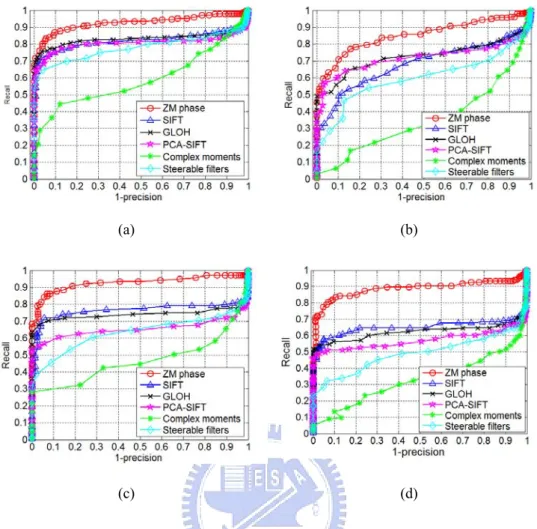
The discriminative power of the new ZM phase descriptor is compared with five other major region descriptors based on the precision-recall criterion using the set of test images given in [12] plus some new images. To match the region pairs, a new matching function based on the ZM phase information is defined. For performance evaluation, important system parameters are taken into consideration, which include (1) region scene types, (2) region descriptor types, (3) region detector types, (4) region overlap error, and (5) transformation types. The experimental results involving more than 15 million region pairs indicate the proposed ZM phase has the best overall performance. Both quantitative and qualitative analyses on the descriptor performances are provided to account for the performance discrepancy.

The chapter is organized as follows. Section 2 introduces the Zernike moment (ZM) transformation and the ZM basis filters. Section 3 proposes the ZM phase descriptor along with a matching function, and discusses the discriminative powers of the ZM magnitude components and the ZM phase components. In Section 4 the discriminative power of the new descriptor is compared with five existing region descriptors based on the precision-recall criterion, while taking important system parameters into consideration. In Section 5 both quantitative and qualitative analyses on the descriptors are provided to account for the descriptor performance discrepancy.

(31)

3.2 Fundamentals of Zernike Moments

Zernike moments (ZMs) have been used in object recognition and image analysis regardless of variations in position, size and orientation [20], [24]-[28]. Basically, the Zernike moments are the extension of the geometric moments by replacing the conventional transform kernel _xm_yn_{with orthogonal Zernike polynomials. The relationships between the}

Zernike moments and geometric moments can be established [39]. The ZM coefficients are the outputs of the expansion of an image function into a complete orthogonal set of complex basis functions {V_nm( , )}ρ θ . Teh and Chin [20] show that among many moment based shape descriptors, Zernike moment magnitude components are rotationally invariant and most suitable for shape description.

The Zernike basis function Vnm (ρ, θ) with order n and repetition m is defined over a unit

circle in the polar coordinates as follows:

( , ) ( )

jm

nm nm

V ρ θ =R ρ e θ_{for ρ ≤ 1, (3.1)}

where {Rnm(ρ)} is a radial polynomial in the form of

s n m n s s nm s m n s m n s s n R ( | |)/2 2 0 _)! 2 | | ( )! 2 | | ( ! )! ( ) 1 ( ) ( − − = + ₋ − ₋ − − =

∑

ρ ρ .

Here n is a non-negative integer and m is an integer satisfying the conditions: n-|m| is even and |m|<n.

The set of basis functions {Vnm (ρ, θ)} is orthogonal, i.e.,

2 1 _* 0 0V nm( , )Vpq( , ) d d n 1 np mq π π ρ θ ρ θ ρ ρ θ = δ δ +

∫ ∫

_with otherwise b a ab 0 1 { = = δ . (3.2)

(32)

The two-dimensional ZMs for a continuous image function f (ρ, θ) are represented by 2 1 _* 2 1 0 0 0 0 1 1 ( , ) ( , ) e jm ( , ) ( ) nm nm nm n n Z π f ρ θ V ρ θ ρ ρ θd d π θ f ρ θ R ρ ρ ρ θd d π π − + + =

∫ ∫

=

∫

. (3.3)

For a digital image function the two-dimensional ZMs are given as

∑ ∑

∈ + = , ( ) unit disk * ₍ _, ₎ ) , ( 1 ρ θ θ ρ θ ρ π nm nm f V n Z . (3.4) The Zernike moments can be viewed as the responses of the image function f (ρ, θ) to a set of quadrature-pair filters {Vnm (ρ, θ)}. To this end, Fig. 3.1 depicts some examples of Vnm( , )ρ θ .

Notice that the real and imaginary functions of each basis function V_nm( , )ρ θ are out of phase by π/2; namely,they form quadrature pairs of filters. In addition, repetition m indicates

m sector cycles of the function values along the azimuth angle θ, while n and m jointly specify a different number of annular patterns of the function.

(a) (b) (c)

(d) (e) (f) Fig. 3.1: Plots of the real part and imaginary part of Vnm (ρ, θ) for a fixed n: (a)V5,1, (b)V5,3, (c)V5,5,

(33)

3.3 Design of A Zernike Moment Phase Based Descriptor

We shall use the ZM phase information to design a novel region descriptor. Let the Zernike moments be sorted by m and n in order. The total number of ZM moments of the same repetition m is equal to

2

N m−

⎢ ⎥

⎣ ⎦+1. Table 3.1 gives the sorted list of the 42 complex ZM

moments for the case where the maximum order N and maximum repetition M are both equal to 12.

The sorted Zernike moments form a feature vector P as follows:

31 11 11 31 [ j , j , , j NM]T NM P= Z eϕ Z eϕ Z eϕ , (3.5)

where Z_nm is the ZM magnitude，and ϕ_nm is the ZM phase. Here the Zernike moments

nm j nm

Z eϕ with m = 0 are not included, since they provide no information regarding the image

matching. Zernike moments with m <0 are not included, either, since they can be inferred

throughZ_n_,₋_m =Z*nm.

TABLE 3.1.LIST OF ZMS SORTED BY nAND m IN SEQUENCE FOR THE CASE WHERE (n m, )=(12,12)

m Moments No. of moments m Moments No. of moments 1 Z₁₁,Z₃₁,Z₅₁,Z₇₁,Z₉₁,Z₁₁_,₁ 6 7 Z₇₇,Z₉₇,Z₁₁_,₇ 3 2 Z₂₂,Z₄₂,Z₆₂,Z₈₂,Z₁₀_,₂,Z₁₂_,₂ 6 8 Z88,Z10,8,Z12,8 3 3 Z₃₃,Z₅₃,Z₇₃,Z₉₃,Z₁₁_,₃ 5 9 Z₉₉, Z₁₁_,₉ 2 4 Z₄₄,Z₆₄,Z₈₄,Z₁₀_,₄,Z₁₂_,₄ 5 10 Z₁₀_,₁₀, Z₁₂_,₁₀ 2 5 Z₅₅,Z₇₅,Z₉₅,Z₁₁_,₅ 4 11 Z11,11 1 6 Z66,Z86,Z10,6,Z12,6 4 12 Z12,12 1

(34)

3.3.1 The Image Description power of the ZM Magnitude Components and the ZM Phase Components

Let the Zernike moments of a reference image and its rotated version be ref nm

Z , rot nm

Z , respectively. Then it is well known that [24], [28]

α jm ref nm rot nm Z e Z ₌ − _{, (3.6)}

where α ∈[0, 2π ] is the rotation angle.

Therefore, the magnitudes of Zernike moments of the two images are the same,

i.e., rot

nm ref

nm Z

Z = , but their phase difference (or phase shift) is given by

α

m Z Z ref nm rot nm nm _⎟⎟ = ⎠ ⎞ ⎜ ⎜ ⎝ ⎛ ≡ Ω arg , 0<Ω_nm ≤2mπ, or (3.7) π α π ϕ ϕ - )mod2 ( )mod2 ( _nmref _nmrot m nm = = Φ , 0<Φ_nm≤2π. (3.8) In the following, under a mixture of rotation, inversion, and flipping operations, the Zernike moments of a reference image can be shown to be rotationally invariant in terms of the magnitudes, but not the phases.

Let a rotated-and-inverted (the inverted is in terms of gray values) image version of the reference image fref (ρ,θ) be denoted by _frot−inv(ρ,θ)=255- _fref(ρ,θ +α)_{. It can readily} shown that their magnitudes are equal: rot inv

nm ref

nm Z

Z = − and their phase difference is given by

[

ϕ ϕ α π

]

π

(

α π

)

π

π ϕ

ϕ - ]mod2 -( - )mod2 - mod2

[ ref m m nm ref nm inv rot nm ref nm nm = = + = Φ − _{. (3.9)}

(35)

Next, let a rotated-and-mirrored version of the reference image _fref( , )_{ρ θ} _{be denoted by}

( , ) ( , ( ))

rot mirror ref

f − ρ θ ₌ f ρ π θ α_{− +} _{. Then it can be shown that their magnitudes also are equal:}

ref nm mirror

rot

nm Z

Z − = _{and their phase difference is given by}

π α π ϕ π ϕ ϕ - )mod2 [2 - ( )]mod2 ( = − = Φ − ref _m nm mirror rot nm ref nm nm . (3.10)

3.3.2 Zernike Moment Phase Descriptor and Its Similarity Measure

From above, it can be seen that the phase information of Zernike moments is more informative than the magnitude information in terms of the discriminative power. Therefore, a new image region descriptor is proposed which is mainly based on the phase components of the feature vector, while the magnitude components are used only as the weighting factors.

Let )Ir( yx, _{and ( , )}_{I x y as the reference and transformed image regions with their}t

respective ZM feature vectors { r i nmr }

r nm

P = Z eϕ and { t i nmt }

t nm

P = Z eϕ . Here the transformed image can be either a rotated version of the reference image or a different image. If there exists a rotation angle αˆ betweenIr(x,y)_{and ( , )}_{I x y , then}t ₍ _ˆ_{) mod(2 )}

nm mα π

Φ − , which

denotes the absolute phase difference between the two image regions after the rotation alignment, is equal to 0; otherwise, Φ −_nm (mαˆ) mod(2 )π is a nonzero value in the interval (0, 2π) and αˆ is simply a putative estimate of a non-existent rotation angle. To derive a reliable estimate using all available phase differences {Φ_nm}, we define a weighted, normalized phase difference to check the existence of a rotation angle αˆ as follows:

(36)

,

ˆ ˆ

min{ ( ) mod(2 ) , 2 ( ) mod(2 )}

r t nm nm nm I I m n m m D w α π π α π π Φ − − Φ − =

∑∑

, (3.11) where ( r - t ) mod(2 ) nm nm nm

Φ = ϕ ϕ π , αˆ is the estimated rotation angle to be described later, and w is a normalized weighting factor of the form _nm

, ( ) r t nm nm nm r t nm nm n m Z Z w Z Z + = +

∑

(3.12)

such that the phase components associated with small magnitudes are weighted less. The weighted, normalized phase difference D_{I I}r_,t lies in the interval [0, 1] and is dimensionless

since it is derived from ratios of angles.

Figs. 3.2(a)-2(d) show a reference coin image and its three variants: a rotated one (with a rotation angle 37.22o), an inverted one, and a mirrored one, as described above. Image matching between the reference and each variant based on either the phase components or the magnitude components of Zernike moments are shown in Figs. 3.2(e) - 3.2(j) where the ZM order (n, m) ranges from (1, 1) to (10, 10). The estimated values of (mαˆ)mod(2π) are colored

in blue and are connected for components with the same m values. The actual phase differences Φ are shown in the red color. On the other hand, the ZM magnitude _nm components for each pair of images are colored in purple. Notice that the magnitude component diagrams are the same for all the three pairs, but the phase component diagrams are different. Therefore, the phase components have a better discriminative power than the magnitude components.

(37)

(a) (b) (c) (d)

(e)ZM phase for (a) and (b) (f) ZM phase for (a) and (c) (g) ZM phase for (a) and (d)

(h) ZM magnitude for (a) and (b) (i) ZM magnitude for (a) and (c) (j) ZM magnitude for (a) and (d) Fig. 3.2: (a) The reference coin image. (b) A rotated variant of the reference coin image (with a rotation angle 37.22o_{). (c) An inverted variant. (d) A mirrored variant. (e)-(g) The diagrams of the ZM phase differences (h)-(j)}

The diagrams of the ZM magnitude components.

3.3.3 Estimation of the Rotation Angle from a Rotated Image

In [29] Kim and Kim represented the rotation angle between an original image and its rotated image through the use of the Zernike moment phase shift as

α π π ϕ π ϕ_nm k _nmr k _nm k_nm m nm = + − + =Φ + = Ω ( 2 ₁ ) ( 2 ₂ ) 2 . (3.13)

They then proposed a probabilistic model P(ˆ) P(ˆ|n,m)

m n nm

α ξ

α =

∑∑

to estimate the rotation

angle α where ξ_nm is the weighting factor proportional to the ZM magnitude Z_nm . For

each possible solution nm _nm

nm k

m m

π

(38)

1 0 1 2 ˆ ˆ ˆ ( | , ) * ( , ) nm m nm nm k P n m k G m m m π α − δ α α σ = ⎧ ⎛Φ ⎞⎫ = _⎨ −_⎜ + _⎟_⎬ ⎝ ⎠ ⎩ ⎭

∑

, a convolution of an impulse train with

a scaled Gaussian kernel, to estimate α. Notice that the estimation is done in discrete angle steps. In order to be accurate, the estimation step size must be as small as possible. Let the estimation step size is 0.01o. For the case where (N, M) = (10, 10), there are 30 generated Zernlike Moments {Znm}. From each fixed Zernike moment Znm an estimator of the rotation

angle is given by nm _nm

nm k

m m

π

αˆ = Φ +2 . There are 30 such estimators. To find the common solution to the rotation angleα using these 30 estimators, a common histogram with a bin size of 360×100 (assuming the estimation step size is 0.01o_{) is used to tabulate the possible}

rotation angle produced by the 30 estimators. Therefore, the total number of histogram bin values computed is 360×100×30 (=1,080,000), which is rather large. In addition, the method may face the ambiguity in multiple peaks in the histogram constructed.

Here a new estimation method of the rotation angle αˆ is proposed, which is implemented in the continuous angle space rather than in the discrete space. The basic idea behind the proposed method for estimating the rotation angle αˆ is to avoid the m _m ambiguities in the value of k . Instead, the rotation angle _nm αˆ can be found from the phase difference using any two adjacent Φ and _nm Φ_n_,_m₋₁,m≠0, through

, 1 , 1 ( 1) ( _nm 2 _nm) ( _{n m} 2 _{n m} ) m m k k α = α− − α = Φ + π − Φ ₋ + π ₋ (3.14) , 1 ( _nm _{n m}₋ ) mod 2π = Φ − Φ , m≠0.

Since m = 1, 2, .., M, n = 1, 2, ..,N, there are

1 ( 1) 2 M m N m = − ⎢ _{⎥ +} ⎢ ⎥ ⎣ ⎦

∑

ways to compute the rotation

(39)

magnitude |Znm|.

An iterative computation of the rotation angle αˆ using all available Zernike moments sorted by m is given below:

The ZM phase-based rotation angle estimation algorithm

Initialization:αˆ₀=0 and c0 = 0 For m = 1, 2, …, M For n = m, m +2, .., m+2 2 N m− ⎢ ⎥ ⎢ ⎥ ⎣ ⎦ π α δ_nm =[(Φ_nm −(m−1)ˆ_m₋₁]mod2 2 r t nm nm nm Z Z w = + End 2 2 , 0 N m m k m m k w s m − ⎢ ⎥ ⎢ ⎥ ⎣ ⎦ + = =

∑

2 2 , 2 , 0 1 N m m k m m m k m k m w s m δ δ − ⎢ ⎥ ⎢ ⎥ ⎣ ⎦ + + = =

∑

) ˆ ( 1 ˆ ₁ ₁ 1 m m m m m m m c s s c α δ α + + = ₋ ₋ − m m m c s c = ₋₁+ End ˆ ˆ_M α α=

(40)

3.4 Experimental Results for Performance Evaluation

We will examine the system performance with respect to important system parameters including (1) region scene types, (2) region descriptor types, (3) region detector types, (4) region overlap error, and (5) transformation types. The region scene types under consideration are the structured and textured scenes. The test images available at the website [30], plus some new images, are used in the experiments. The transformation types considered here contain the common photometric transformations (blur, illumination, noise, and JPEG compression) and geometric transformations (rotation, scaling, translation, and viewpoint). Fig. 3.3 shows the representative test image pairs taken for the textured and structured scenes. In regard to the region descriptor types we include the proposed ZM phase and five popular descriptors: SIFT, GLOH, PCA-SIFT, steerable filters, and complex moments. In the beginning of the experiment, we need to choose a region detector in order to extract the regions of interest from the given image. Here we decide to choose either MSER detector or Hessian-affine detector. Once the region detector type is decided, the program codes available at the website [30] are used to obtain (a) regions of interest, (b) the dominant orientation in a region image and (c) the descriptor feature vectors of SIFT, GLOH, PCA-SIFT, steerable filter and complex moment for each region of interest. Then we run our program codes to generate our ZM phase descriptor and to calculate the similarity measures and generate the precision-recall curves to evaluate the descriptor performances, as done in [12]. Totally, there are 8 types of transformations, 2 types of scenes, and at least 4 image pairs for each transformation. On the average, one image pair generates 250,000 (= 500×500) region pairs for matching. All together the experiments involve more than 15 million region pairs.

(41)

(a) bikes

(blur) (b) tree (blur) (c) Leuven (lighting)

(d) bush 1

(lighting) (nonlinear lighting) (e) Leuven (nonlinear lighting) (f) bush 1

(g) Chinese compound (noise) (h)Japanese garden

(noise) (i)UBC (JPEG)

(j) garden

(JPEG) (viewpoint) (k) graffito (l) wall brick (viewpoint)

(m) castle

(rotation) (rotation) (n) flower (m) Pentagon (scaling)

Fig. 3.3: Representative test image pairs taken from the textured and structured scenes under a specified photometric or geometric transformation.

TABLE 3.2THE TYPICAL FEATURE VECTOR DIMENSIONS OF THE SIX DESCRIPTORS

Descriptor SIFT GLOH ZM phase PCA- SIFT complex

moments

steerable filters Feature

dimensionality 128 128 42 36 15 14

3.4.1 Performance Evaluation Criteria – PR curve

For region matching, the extracted regions of the reference and transformed images are examined for (a) their distance measure and (b) their spatial overlap error under the applied transformation. There are three strategies for region matching proposed in [12]: (a) the

(42)

threshold-based matching, (b) the nearest-neighbor-based matching, and (c) two-nearest- neighbor-based matching. Although these three matching methods are functionally different, their ranking results of the performances of the various descriptors are virtually the same; the first one is generally recommended [12], [38]. Therefore, we adopt the threshold-based matching strategy in which the distance measure between a region pair is compared to a given distance threshold, Dt.

On the other hand, the region overlap error is represented by the overlap ratio between the region intersection area and the region union area under the known planar homography [12], [31], that is, O 1 (A HTBH)/(A HTBH)

e = − ∩ ∪ , where A and B are the two matching

regions and H is the given homograph between the two region patches. A region pair is called a match if it passes the region similarity test, namely, the distance measure between the image pair does not exceed the distance threshold Dt; otherwise, no match is found. A match is said

to be correct, if the region pair also passes the region overlap test given by Oe< Ot for a given

overlap error threshold Ot. A match is said to be false, if the pair fails the region overlap test.

Sometimes, with a tight overlap error threshold, say Ot = 0.1, even though the two regions

pass the region similarity test, but they fail the region overlap test due to Ot <Oe<1. It seems

not very fair to call such a pair a false match when compared to a typical false match whose region overlap error Oe is equal to 1; namely, the two regions do not intersect and are,

therefore, not related at all. Hereafter, a matching pair with a region overlap error in between such that Ot <Oe<1 is considered as a “don’t care” pair. In other words, the new definition of a

false match is a match that passes the region similarity test and its region overlap error Oe

must be equal to 1.

It is important to realize a fixed distance threshold cannot be used to evaluate the descriptor performances. Instead, a precision-recall (PR) curve, created by varying the

(43)

distance threshold, must be used.

Recall is the ratio of the number of correct matches to the number of corresponding region pairs satisfying the region overlap test: Oe< Ot.

recall = ences correspond # matches correct # . (3.15)

Precision is the ratio of the number of correct matches to the total number of correct and false matches: 1- precision = matches false # matches correct # matches false # + . (3.16)

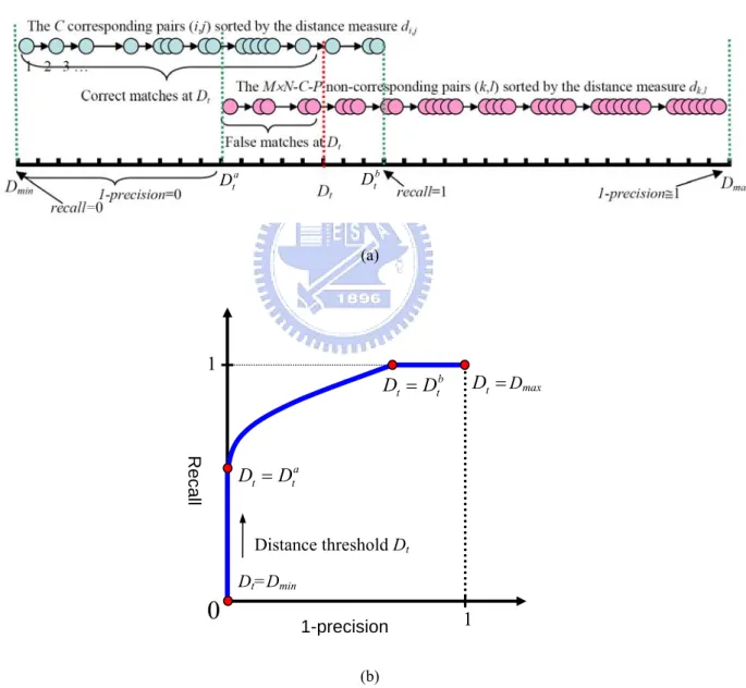
Fig. 3.4 depicts a PR curve generation process. Assume there are M, N regions detected in the reference and transformed images, respectively. The regions in the two images form M×N

matching region pairs. Among these M×N pairs let the number of corresponding region pairs,

which are each with a region overlap error Oe smaller than the specified bound Ot, be C. Also,

let the number of the “don’t care” pairs be P. Now sort the C corresponding pairs and the

M×N-C-P non-corresponding pairs, respectively, by their distance measures di,j in an

ascending order. The range of distance measures for the set of C corresponding pairs generally overlaps with that of the set of non-corresponding pairs. Start to increase the distance threshold Dt from the minimum value Dmin to the maximum value Dmax. The recall value is

initially equal to zero, so is the value of (1-precision). As Dt passes over Dmin, more and more

correct matches occur and the recall value is increasing, while the (1-precision) value remains 0 since there have been no false matches so far. When Dt reaches the minimum distance

measure a t

D of the non-corresponding region pairs, false matching pairs begin to appear and the value of 1-precision is increasing from 0. Notice that the recall is always monotonically

(44)

increasing and reaches 1 when the distance threshold is equal to the maximum distance measure b

t

D of the C corresponding region pairs. At the end, when the distance threshold is

equal to Dmax, the (1-precision) value approaches 1. Be aware that the (1-precision) value is

monotonically increasing when Dt is sufficiently large, but it may decrease at the early stage,

if the relative growth rate of false matches is smaller than that of the correct matches.

(a)

(b)

Fig. 3.4: The PR curve generation process. (a) The correct matches and false matches associated with a varying distance threshold Dt . (b) The generated PR curve.

Recall 1-precision

0

₁ 1 a t t D =D b t t D =D Dt =Dmax Dt=Dmin Distance threshold Dt a t D b t D

(45)

3.4.2 Evaluation on Region Detector Types and Region Overlap Error

As mentioned above, the best two region detectors, MSER and Hessian-affine, are reported in [11]. We shall present the evaluation results for these two detectors side by side.

Fig. 3.5 and Fig. 3.6 show the region detection results for both textured and structured scenes, and the two curves about the relation between recall and region overlap error and that between the number of correct matches and region overlap error using Hessian-affine regions and MSER regions, respectively. There are around 400 regions extracted by either detector. The number of correct matches and the number of correspondences for each overlap error are computed for a single section of overlap errors ranging from the previous one to the current one. For instance, the score for 20 percent is computed for the overlap error interval from 10 percent to 20 percent. Also, the recall values are calculated, by keeping the precision at 0.5, as done in [12].

We observe that the top black line, which shows the number of region correspondences dictated by the given overlap error bound Oe, bounces back at overlap error 40%. This is due

to a natural increase in the region correspondences at the given higher region overlap error bound, resulting in “one-to-many” or “many-to-one” overlapped region pairs extracted from the reference and sensed scenes. Usually these new corresponding region pairs are less similar when compared to those at a smaller overlap error bound, causing a drop in the number of new correct matches. On the other hand, for a small overlap error bound the correspondences are mostly the “one-to-one” overlapped region pairs.

(46)

(a) Hessian-affine regions (b) MSER regions

(c) (d)

(e) (f) Fig. 3.5: Evaluation for different overlap errors for structured scene. (a)–(b) Detected Hessian-affine

regions and MSER regions under viewpoint change for structured graffti scene. (c)-(d) The number of correct matches vs. the overlap error. Also, the top black line shows the number of region correspondences detected. (e)-(f) Recall vs. the overlap error.

(47)

(a) Hessian-affine regions (b) MSER regions

(c) (d)

(e) (f) Fig. 3.6: Evaluation for different overlap errors for textured scene. (a)–(b) Detected Hessian-affine

regions and MSER regions under viewpoint change for textured brick scene. (c)-(d) The number of correct matches vs. the overlap error. Also, the top black line shows the number of region correspondences detected. (e)-(f) Recall vs. the overlap error.

(48)

We observe that the proposed ZM phase descriptor has a higher recall vs. region overlap error curve than other descriptors for the region overlap error in the interval [0.1, 0.4] for both sets of Hessian-affine and MSER regions. The portion of curve is less meaningful when Ot

gets larger. This is because when Ot gets larger, the corresponding regions are less similar, as

indicated in Figs. 3.7. As mentioned above, when the overlap error bound increases over 0.4, the intersection area of these new corresponding region pairs becomes smaller, resulting in the drop of the number of correct matches and the decrease in the recall value under a fixed precision level (0.5 in this case). At a large overlap error bound the Zernike phase maintains the same tight control on the similarity matching of the new corresponding pairs based on the orthogonal moment features, so the increase in the new correct matches is rather small. On the other hand, SIFT and GLOH have less stringent control on the similarity measure based on the 8-gradient orientation bin tabulation on the 4×4 location grid, so there are more new correct matches when the overlap error bound increases.

Oε= 0.1 Oε= 0.2 Oε= 0.3 Oε= 0.4 Oε= 0.5 Oε= 0.6

Fig. 3.7: The examples of the detected region pairs with different overlap errors Oε ranging from 0.1 to 0.6.

The ellipses indicate the region boundary with blue color and red color for reference region A and the transformed region given by HT_{BH, respectively. The cross symbols show the key point positions.}

應用不變量澤爾尼克矩描述元進行影像之表示、比對及辨識

國

立

交

通

大

學

資 訊 學 院

資訊科學與工程研究所

博

士

論

文

應用不變量澤爾尼克矩描述元

進行影像之表示、比對及辨識

Image Representation, Matching, and Recognition

Using Invariant Zernike Moment Descriptors

研 究 生：孫 樹 國

指導教授：陳 稔 教授

應用不變量區域描述元進行影像之表示、比對及辨識

Image Representation, Matching, and Recognition

Using Invariant Zernike Moment Descriptors

研 究 生：孫樹國 Student：Shu-Kuo Sun

指導教授：陳 稔 Advisor：Zen Chen

國 立 交 通 大 學

資 訊 學 院

資訊科學與工程研究所

博 士 論 文

進行影像之表示、比對及辨識

研究生： 孫樹國 指導教授： 陳稔博士

國立交通大學

資訊學院

資訊科學與工程研究所

摘 要

Image Representation, Matching, and Recognition

Using Invariant Zernike Moments Descriptors

Student：Shu-Kuo Sun Advisor：Dr. Zen Chen

Institute of Computer Science and Engineering

College of Computer Science

National Chiao Tung University

ABSTRACT

ACKNOWLEDGEMENTS

Table of Contents

LIST OF FIGURES

LIST OF TABLES

Introduction

1.1 Problems Statement

1.2 Sketch of the Work

1.3 Contribution of the Work

1.4 Dissertation Organization

Previous Work

2.1 Region detectors and descriptors

∑∑

∑∑

2.2 Logo Recognition

2.3 View Registration

A Zernike Moment Phase Based Descriptor for

Local Image Representation and Matching

3.1 Introduction

3.2 Fundamentals of Zernike Moments

∑

∫ ∫

∫ ∫

∫

∫

∑ ∑

3.3 Design of A Zernike Moment Phase Based Descriptor

α

[

]

(

)

∑∑

∑

∑∑

∑

∑

∑

∑

3.4 Experimental Results for Performance Evaluation

資訊學院

研究生：孫樹國

指導教授：陳稔教授

研究生：孫樹國 Student：Shu-Kuo Sun

指導教授：陳稔 Advisor：Zen Chen

國立交通大學

資訊學院

博士論文

研究生：孫樹國指導教授：陳稔博士

摘要