應用於匯流排矩陣系統之仲裁器權重調整演算法

國立交通大學

電子工程學系電子研究所碩士班

碩士論文

應用於匯流排矩陣系統之仲裁器權重調整演算

法

A Weight Tuning Algorithm for Arbiters in Bus

Matrix Systems

研究生： 陳匡緯

指導教授： 周景揚博士

應用於匯流排矩陣系統之仲裁器權重調整演算

法

A Weight Tuning Algorithm for Arbiters in Bus

Matrix Systems

研究生：蔡孟家 Student: Kuang-Wei Chen

指導教授：周景揚博士 Advisor: Dr. Jing-Yang Jou

國立交通大學

電子工程學系電子研究所碩士班

碩士論文

A Thesis

Submitted to Department of Electronics Engineering & Institute

of Electronics College of Electrical and Computer Engineering

Institute of Electronics

National Chiao Tung University

in Partial Fulfillment of the Requirements for the Degree of

Master of Science in Department of Electronics Engineering

February 2009

HsinChu, Taiwan, Republic of China

應用於匯流排矩陣系統之

仲裁器權重調整演算法

研究生：陳 匡 緯

指導教授：周 景 揚 博士

國 立 交 通 大 學

電 子 工 程 學 系 電 子 研 究 所 碩 士 班

摘

要

A Weight Tuning Algorithm for Arbiters

in Bus Matrix Systems

Student:

Kuang-Wei

Chen Advisor:

Dr.

Jing-Yang

Jou

Department of Electronics Engineering

Institute of Electronics

National Chiao Tung University

Abstract

Arbiters are mandatory components on SoC bus systems to resolve contentions of bus access requests from different IP cores. Lottery-based arbitration algorithms are probabilistic and efficient arbitration algorithms. However, lottery-based arbitration algorithms need a weight tuning mechanism to help them simultaneously meet both the real-time and bandwidth requirements. In this thesis, we propose a new weight tuning algorithm, named MC weight tuning algorithm, which considers multiple buses at one time. The experimental results show that MC weight tuning algorithm helps lottery-based arbitration algorithms efficiently meet bandwidth requirements of IP cores in bus matrix systems.

Acknowledgment

Contents

List of Tables ...viii

Chapter 1 Introduction... 1

1.1 Introduction ... 1

1.1.1 Shared bus architecture... 2

1.1.2 Bus matrix architecture... 3

1.2 The purpose and challenge of arbiter ... 6

1.3 The focus of our work ... 7

1.4 Thesis organization... 7

Chapter 2 Preliminary... 8

2.1 Traffic models of masters ... 8

2.2 Lottery-based arbitration algorithms ... 11

2.3 Local-bus weight tuning algorithm ... 13

2.4 Motivation ... 18

2.4.2 Bus matrix architecture with local-bus weight tuning... 22

Chapter 3 The proposed Algorithm ... 28

3.1 A weight tuning algorithm with multi-bus consideration... 28

3.1.1 Notations... 30

3.1.2 The details of MC weight tuning algorithm ... 33

Chapter 4 Experimental Results ... 40

4.1 Experiment setup ... 40

4.2 Experiment 1 ... 41

4.3 Experiment 2 ... 46

Chapter 5 Conclusions and Future Work... 50

5.1 Conclusions ... 50

List of Figures

Figure 1 : An example of single shared bus architecture... 2

Figure 2 : A simple representation of Figure 1 ... 3

Figure 3 : An example of bus matrix architecture ... 5

Figure 4 : A simple representation of Figure 3 ... 5

Figure 5 : A probability based model is used to model the behavior of MM ... 5

Figure 6 : D type master (beat number = 4; interval time = 17)... 9

Figure 7 : D_R type master (beat number = 4; interval time = 17; Rcycle = 10)... 10

Figure 8 : ND_R type master (beat number = 4; interval time = 17; Rcycle = 10)... 10

Figure 9 : The Lottery communication architecture ... 11

Figure 10 : An example of Lottery ... 12

Figure 11 : Bandwidth allocation under different tickets assignment ratio... 14

Figure 12 : An example of single share bus architecture with four masters... 15

Figure 13 : The bandwidth allocation under three different ticket assignments... 15

Figure 14 : The simple flow of local-bus weight tuning ... 17

Figure 15 : An example of Bus matrix architecture ... 19

Figure 16 : Independent buses architecture separated from Figure 15... 19

Figure 17 : An example of the request limitation of masters ... 22

Figure 18 : An example shows the difference between IB and Figure 17... 22

Figure 20 : An example of a MM with the request ratio equaling to 1:4 ... 25

Figure 21 : An MM misses or meets all bandwidth requirements... 26

Figure 22 : A missed bandwidth requirement on a bus induces all bandwidth missed on other buses ... 27

Figure 23 : The flow chart of MC weight tuning algorithm ... 30

Figure 24 : The bus matrix system of the example of MC weight tuning ... 34

Figure 25 : The flow of global-bus weight tuning... 36

Figure 26 : An example of implementation of a bus matrix system on SoC Designer ... 41

Figure 27 : The bus matrix architecture of experment1 ... 42

Figure 28 : The figure of Table 13... 45

Figure 29 : Bus matrix architecture with two buses ... 47

Figure 30 : Bus matrix architecture with three buses ... 47

Figure 31 : Bus matrix architecture with four buses ... 48

List of Tables

Table 1 : The traffic models of Figure 12 ... 15

Table 2 : The traffic model of Figure 15... 20

Table 3 : The modified traffic model of Figure 16 ... 20

Table 4 : The bandwidth requirement of Figure 15 and Figure 16 ... 21

Table 5 : The simulation result of Figure 15 and Figure 16 ... 21

Table 6 : The traffic model of Figure 19... 24

Table 7 : The simulation result of Figure 19 with the local-bus weight tuning... 24

Table 8 : The traffic model of Figure 24... 34

Table 9 : The ticket assignment and bandwidth allocation after inner loop terminated ... 35

Table 10 : Table 9 with more information ... 36

Table 11: The simulation result of example Figure 24 by MC weight tuning algorithm .... 39

Table 12 : The traffic model of Figure 27... 43

Table 13 : The number of success case under different weight tuning algorithm ... 44

Chapter 1

Introduction

1.1 Introduction

With the technology scaling and the level of system integration, system-on-chip (SoC) design is widely adopted in today’s design methodology. It integrates a number of intellectual property (IP) components, such as processor, memory, DSP, and ASIC, into a single chip to meet the design specification. Since those components need to communicate each other for data exchange, the on-chip communication architecture has a significant impact on the system performance. Many on-chip communication architecture topologies are proposed to facilitate the data exchange between components in a system. The shared bus based architecture is very popular in the designs with moderate complexity because of

which limits the system performance[1, 2]. In order to resolve the bandwidth limitation of shared bus architecture, the bus matrix architecture is used to provide higher system parallelism. In the following two sections, we briefly introduce this two on-chip communication architectures.

1.1.1 Shared bus architecture

Shared bus is one of widely used on-chip communication architectures. The communication is commonly built through the shared media called bus. Shared bus is acted as a shared channel between components and then components communicates with each other through the bus [1, 3].

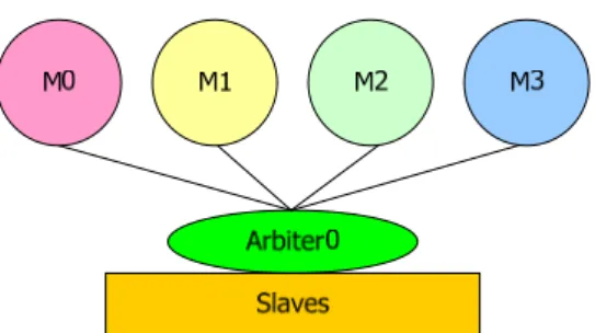
Two categories of components are connected through the shared bus. Master components initiate data transaction requests (either read or write transactions), and slave components respond to corresponding requests with proper data transactions. A simple example of single shared bus architecture is shown in Figure 1. There are three masters, M0, M1, and M2, and two slaves, S1 and S2. Masters initiate requests and slaves response the corresponding requests through single shared bus [4-11]. Figure 2is a simplified graph ofFigure 1.

M0 M1 M2

Arbiter0 Slaves

Figure 2 : A simple representation of Figure 1

More than one master can initiate requests at the same time on the shared bus system; however, only one master can be granted to bus access. An arbiter is required to decide which master can be granted without bus conflicts. Since the arbiter decides which master is the current bus owner to avoid bus conflicts, the arbiter influences the system performance significantly. As a result, the arbiter is indeed an important component of shared bus architecture.

Since the communication channel is shared, the hardware cost for shared bus architecture is relatively lower than other communication architectures [12, 13]. However, the shared bus architecture can only support limited bandwidth which is not suitable for the current high performance systems.

1.1.2 Bus matrix architecture

In order to achieve higher performance and support larger bandwidth requirement for high performance systems, a different communication architecture, bus matrix architecture, is proposed [1, 2]. It is a combination of shared bus and point-to-point connection structure between components to support higher level of parallelism. The parallel buses provide a

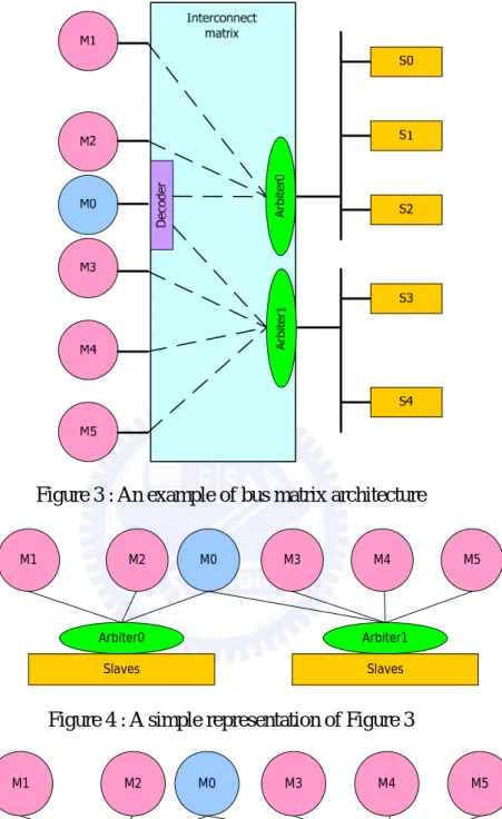
In this architecture, each master connects with each slave system through the separate bus. Each slave system is a shared bus structure where one or more slaves are connected. A simple example of bus matrix architecture with two slave systems is shown in Figure 3. Masters on the left connect with slave systems on the right through the interconnect matrix. One slave system consists of S0, S1, and S2, and the other slave system consists of S3 and S4. Figure 4 is a simplified graph of Figure 3.

Since, a master can connect with one or many slave systems in bus matrix architecture, we classify the masters according to the type of connection. A master which connects with more than one slave systems is called multi-connection master (MM). Otherwise, a master which connects with only one slave systems is called single-connection master (SM). A decoder is required for each MM to determine the data transfer sent to which slave system. For example, as shown in Figure 3, M0 which connects to two slave systems is an MM and M1 which connects to only one slave system is an SM.

Since an MM can have different traffic behavior on each slave system, we use a probability symbol to represent the request rate. As shown in Figure 5, for example, if M0 initiates a request, the request has 40% probabilities to bus 0, and 60% probabilities to bus 1. The “r40%” means that the new initiated request has 40% probabilities to this bus. The sum of probabilities of each bus is 100%. The request probabilities are called request ratio. In other words, the request ratio of M0 on bus 0 is 40%, the request ratio of M0 on bus 1 is 60%.

Figure 3 : An example of bus matrix architecture M1 M2 M0 Arbiter0 Slaves M3 M4 M5 Arbiter1 Slaves

Figure 4 : A simple representation of Figure 3

M1 M2 M0 Arbiter0 Slaves M3 M4 M5 Arbiter1 Slaves r40% r60%

Without loss of generality, a master cannot initiate a new request before the previous request is not completed. While dealing with the requests of MM, the arbitration strategy on each slave system should consider the communication behavior of other slave systems [14, 15]. It becomes more complicated to design the arbiter. In Figure 5, for example, M0 can access both of two slave systems where any pending request of one side would suspend the request of the other side. Since the traffic behavior of multi-connection masters are more complicated, the arbiter becomes more difficult to design for bus matrix architecture.

Comparing with shared bus architecture, bus matrix architecture can provide parallel access paths at one time. As shown in Figure 3 and Figure 4, M0, M1, M2, S0, S1, and S2 can be regarded as a shared bus system called bus 0, M0, M3, M4, M5, S3 and S4 can be regarded as another shared bus system called bus 1. If M1 and M3 both have pending requests, the requests of M1 and M3 can be simultaneously granted without bus conflict. Because of parallel access paths, bus matrix architecture can support larger bandwidth requirement that higher performance system needs than shared bus architecture.

1.2 The purpose and challenge of arbiter

Arbiters play an important role in on-chip communication architectures. Because of the resources limitation, one shared resource can be used by only one component at one time. For example, only one master can be granted to access bus at one time on shared bus architecture, or one slave system can serve only one master at one time on bus matrix architecture. There are many contentions between many requests when different masters initiate its request at the same time. Because of the limitation and contention, we need a component that can decide which pending request of masters can be granted to use resources, that is arbiter. When there is contention occur between some pending requests,

the arbiter must decide only one of them can be granted.

Besides, the master often has the real-time requirements and bandwidth requirements. The arbiter has very important impact on whether those requirements are met or missed because the arbiter decides granted order of requests. It is a challenge for arbiters to meet different requirements simultaneously because masters have diverse traffic behavior.

1.3 The focus of our work

With local-bus weight tuning algorithm, lottery-based arbitration algorithms can meet most bandwidth and real-time requirements simultaneously on single shared bus architecture [4, 8, 9, 16-24]. But we show that local-bus weight tuning algorithm does not work well on bus matrix system comparing with single share bus architecture. We propose an algorithm called MC weight tuning algorithm. MC weight tuning algorithm helps lottery-based arbitration algorithms meet most bandwidth requirements on bus matrix architecture.

1.4 Thesis organization

The remainder of this thesis is organized as follows. The lottery-based arbitration algorithms and an existing weight tuning algorithm proposed in [16] are briefly introduced in Chapter 2. Chapter 3 presents the detail of the proposed weight tuning algorithm, MC weight tuning algorithm. Experimental results are reported in Chapter 4. Finally, we conclude this thesis in Chapter 5.

Chapter 2

Preliminary

We introduce previous works in this chapter. First, we briefly introduce the traffic models. Then, lottery-based arbitration algorithms and local-bus weight tuning algorithm are introduced briefly. Finally, we show some motivational examples for our weight tuning algorithm.

2.1 Traffic models of masters

Four parameters are defined to describe the behaviors of a master. The first parameter of a request is the beat number. For example, if the beat number of a request is 4, it means that it is a 4-beat transaction. In other words, the request needs 4 cycles to complete it works. Second, the time of next request can be initiated is determined as the interval time. For example, if the interval time is 17, the next request initiates after 17 cycles. Third, the real-time requirement is represented as Rcycle which is the dead-line of a request. For

example, if the Rcycle is 10, the request must complete in 10 cycles. At last, we classify three high abstract-level traffic types to emulate the masters behavior [24]. That is D type master, D_R type master, and ND_R type master. The behavior of three different type masters is shown in the following.

z D type (D for dependency):

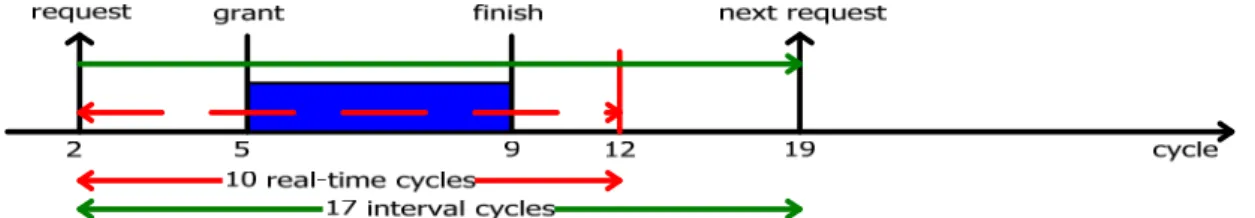
The D type master has no real-time requirement. The time of the D type master initiating a request depends on the finish time of the previous request. In Figure 6, the beat number is 4 and the interval time is 17. If a request is initiated at cycle 2 and granted at cycle 5, the request is completed at cycle 9. The next request is initiated at cycle 26 which is 17 cycles later than the finish time.

Figure 6 : D type master (beat number = 4; interval time = 17) z D_R type (D for dependency, R for real-time):

The behavior of the D_R type master is the same as the D type master except the real-time requirement. Requests of the D_R type master has real-time requirement. In Figure 7, we use the same parameters used in Figure 6 as an example. Because of the real-time requirement, a new parameter, Rcycle, is added in Figure 7. Rcycle is 10 cycles in the example. The first request is also initiated at cycle 2 and the request must be completed before cycle 12 because of the Rcycle is 10 cycles. It is a real-time violation, if the request is not completed

Figure 7 : D_R type master (beat number = 4; interval time = 17; Rcycle = 10) z ND_R type (ND for non-dependency, R for real-time):

The ND_R type master is another kind of master with the real-time requirement. The behavior of ND_R type master is similar to D_R type master except on one thing. The time of the ND_R type master initiating a request does not depend on the finish time of the previous request. Actually, the time of the ND_R type master initiating a request depends on the initiated time of the previous request. In other words, the ND_R type masters initiate requests periodically. In Figure 8, the same parameters are used in Figure 7. Since the interval time is at cycle 17 and the initiated time of the first request is at cycle 2, the second request is initiated at cycle 19, which directly depends on the initiated time of the first request.

Figure 8 : ND_R type master (beat number = 4; interval time = 17; Rcycle = 10) There is a limitation for all masters. If a master had initiated a request, it cannot initiate a new request when the previous request has not been finished. For example, a state machine is involved by a master. The master begins next state after previous state is completed. In other words, all masters are in serial execution.

2.2 Lottery-based arbitration algorithms

Lottery-based arbitration algorithms are probabilistic arbitration algorithm [16, 17, 24].It stochastically grants one of the contending masters according to the ticket assigned to them, either statically or dynamically. Each master holds a number of tickets for lottery-based algorithms. When a bus contention occurs, the lottery manager accumulates tickets of masters. According the tickets assignment, lottery manager probabilistically choose a master granted to access bus. As shown in Figure 9, there are four masters and each of them has a number of lottery tickets as the probability of bus granted. First, the lottery manager accumulates tickets of masters which has pending request. Then the lottery manager probabilistically chooses a master granted to access the bus from all contending masters. In other words, the lottery tickets act as the weight and lottery-based arbitration algorithms are weighted random arbitration algorithm to grant a master while contention.

Let the set of masters, M , M , ..., M , and each of them has _{1 2 n} t , t , ..., t tickets _{1 2 n}

respectively. A set of Boolean variables, r , r , ..., r , represents the corresponding _{1 2 n}

pending request. r is 1 if _i M has pending requests. Otherwise, _i r is 0. _i

The first step, the lottery manager accumulates the total tickets of masters which has pending requests, given by

1 n j j j T r t =

=

∑

[

)

[

)

1 1 1 , i i k k k k k k r t r t + = = ⎡ ⎞ ⎟ ⎢⎣

∑ ∑

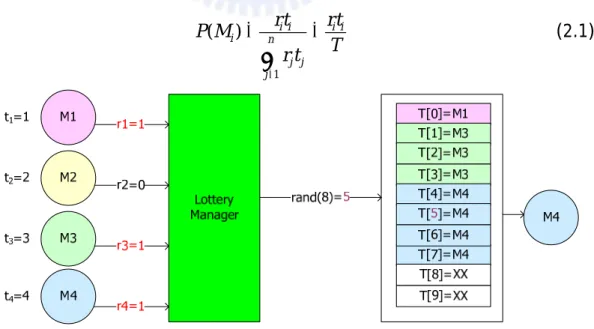
M ₊ is granted. In Figure 10, for example, there are four masters, M1, M2, M3, and M4, and hold 1, 2, 3, and 4 tickets respectively. Three of them have pending requests, M1, M3, and M4, and the lottery manager accumulates their tickets

1 1 0 3 4 8 n j j j T r t = =

∑

[

)

1 1 2 2 3 3 4

r t +r t +r t = and r t_{1 1}+r t_{2 2}+r t_{3 3}+r t_{4 4} = , and then the bus is granted to M4. The 8 probability of M granted to access the bus is shown in Equation2.1. _i

1 ( ) i i i i i n j j j rt rt P M T r t = = =

∑

Since tickets act as granted probabilities of each master for lottery-based arbitration algorithms, ticket assignment is important to system performance. Lottery-based arbitration algorithms need additional algorithm to assign tickets to each master. The additional algorithm is called weight tuning algorithm. We introduce a weight tuning algorithm in the following section.

2.3 Local-bus weight tuning algorithm

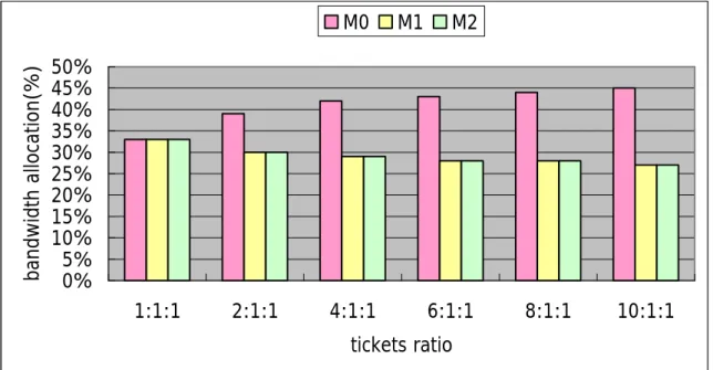
The lottery-based arbitration algorithms need a weight tuning algorithm to result proper ticket assignment for all masters. A weight tuning algorithm can result tickets for each master. Proper ticket assignment makes masters meet their requirements as many as possible. By Equation2.1, tickets can decide grated probabilities for each master, and grated probabilities can obviously affect allocated bandwidth of each master. In other words, tickets have strong impact on bandwidth allocation for each master. For example, a shared bus system has three masters (named M0, M1, and M2) with same traffic models. We simulate with different ticket assignments and respective bandwidth allocation is shown in Figure 11. The notation “10:1:1” means that M0 has tickets ten times larger than M1; and also ten times larger than M2. In Figure 11, it is easily observed that different ticket assignments result totally different bandwidth allocations. The weight tuning algorithm redistributes tickets between masters and result proper ticket assignment for masters. Masters with proper ticket assignment meet their requirements as many as possible.

0% 5% 10% 15% 20% 25% 30% 35% 40% 45% 50% 1:1:1 2:1:1 4:1:1 6:1:1 8:1:1 10:1:1 tickets ratio band wid th allo cat io n(%) M0 M1 M2

Figure 11 : Bandwidth allocation under different tickets assignment ratio

Finding an efficient weight tuning algorithm is a difficult challenge. Most of requirements can be met by ticket assignment resulting from an efficient weight tuning algorithm. In Figure 12 and Table 1, an example shows that why an efficient weight tuning algorithm is a difficult challenge. There are four masters with their traffic models in Table 1. Lottery algorithm with total 1024 tickets is used in Figure 12. We simulate with three different tickets assignments, and simulation results are shown in Figure 13. The notation “252:143:220:409” in Figure 13 means M0 has 252 tickets, M1 has 143 tickets, M2 has 220 tickets, and M3 has 409 tickets. Comparing with three different ticket assignments, we only move the tickets from M0 to M2, but allocated bandwidth of all masters are changed. Bandwidth allocation is totally changed when we redistribute tickets of two masters. When a weight tuning algorithm redistributes tickets between masters, the bandwidth allocation is disordered and not easily predictable.

Figure 12 : An example of single share bus architecture with four masters Table 1 : The traffic models of Figure 12

Type Beat Interval M0 D 32 2 M1 D 16 4 M2 D 8 8 M3 D 8 8 54% 38% 17% 21% 12% 20% 17% 21% 25% 25% 25%25% 0% 10% 20% 30% 40% 50% 60% 252:143:220:409 126:143:346:409 63:143:409:409 tickets ba nd width a lloc ation M0 M1 M2 M3

For single shared bus architecture, an efficient weight tuning algorithm, local-bus weight tuning algorithm, is proposed in [16]. Local-bus weight tuning algorithm results proper tickets for each master and masters can meet most of their requirements. The simple flow of local-bus weight tuning algorithm is shown in Figure 14. At first, the local-bus weight tuning algorithm analyzes the simulation result according the bandwidth allocation of each master. If a master gets bandwidth more than its requirement, it is grouped into Smore. If a master gets bandwidth less than its requirement, it is grouped into Sless. If a

master gets bandwidth almost equal to its requirement, it is grouped into Smet. The master

in Smore who gets the most bandwidth than its requirement is called Mmost. The master in

Sless who gets the least bandwidth than its requirements is called Mleast. Each master in Sless

gets insufficient bandwidth because each of them does not have enough tickets. If the master does not meet its bandwidth requirement, the local-bus weight tuning algorithm increases its tickets. When tickets of a master are increased, the granted probability is increased and the master can get more bandwidth than before. The local-bus weight tuning algorithm redistributes the tickets of masters in Smore and Sless, and tries to meet bandwidth

requirements of each master.

The local-bus weight tuning algorithm is efficient for single shared bus system. Lottery-basd arbitration algorithms with local-bus weight tuning algorithm in single shared bus system can meet hard real-time requirements and bandwidth requirements simultaneously with very high successful probability [24].

2.4 Motivation

In our thesis, we choose lottery-based arbitration algorithms as our arbitration algorithm of bus matrix architecture. With the evolution of process, more and more SoC systems need bus matrix architecture to deal with the complex communication between massive components. Since the lottery-based arbitration algorithms meet the hard real-time and bandwidth requirement simultaneously with high successful probability, using the lottery-based arbitration algorithms for bus matrix architecture is a good choice.

In this thesis, we find how to result proper ticket assignment for bus matrix architecture because we choose lottery-based arbitration algorithms as our arbitration algorithm. Proper ticket assignment of masters is important to lottery-based arbitration algorithms because it makes masters meet their requirements as many as possible. A weight tuning algorithm is needed for bus matrix architecture. Local-bus weight tuning algorithm produces proper ticket assignment for single shared bus architecture. In following, two methods are introduced that try to achieve our goal, finding proper ticket assignment for bus matrix architecture.

2.4.1 Model bus matrix architecture by shared bus architecture

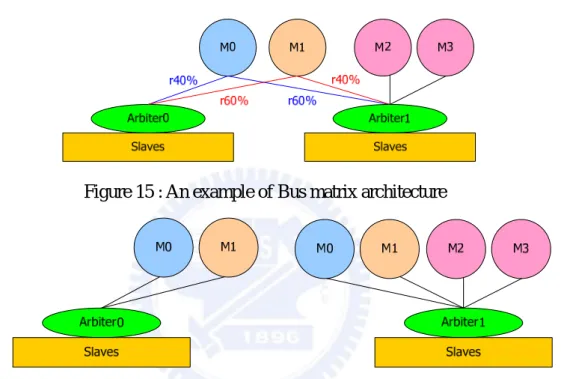
Since lottery-based arbitration algorithms often use local-bus weight tuning algorithm before, we try to the use same weight tuning algorithm for bus matrix architecture. Because local-bus weight tuning algorithm used to be with single shared bus architecture, bus matrix architecture is intuitionally separated into many “single shared bus architecture”. In other words, bus matrix architecture is modeled by shared bus architecture. As shown in Figure 15 and Figure 16, bus matrix architecture has two buses, but two buses are

separated into two “single shared bus architecture” intuitionally. Bus 0 is single shared bus architecture, and bus 1 is single shared bus architecture, too. The traffic behavior of M0 on the bus 0 is independent to M0 on the bus 1. In other words, two buses are independent to each other. Therefore, the architecture which separates from bus matrix architecture is called “independent buses” or “IB” for simplification.

Figure 15 : An example of Bus matrix architecture

Figure 16 : Independent buses architecture separated from Figure 15

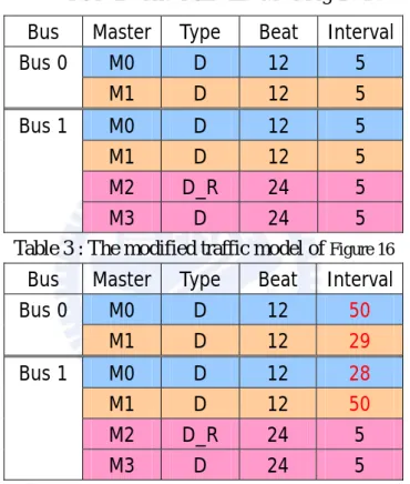
After independent buses architecture is generated, traffic model of bus matrix architecture has to be modified for independent buses architecture. In Figure 15, for example, the request ratio of M0 is 40% on the bus 0. It means that M0 on the bus 0 holds about 40% of total traffic amount of M0. In Figure 16, M0 on the bus 0 holds 100% of total traffic amount of M0. To make the behavior of independent buses architecture more similar to bus matrix architecture, traffic model of bus matrix has to be modified. The traffic model of Figure 15 is shown in Table 2. We simulate the bus matrix system and record the traffic

comparing with bus matrix architecture. We modify the parameters of Table 2 continuously until the traffic behavior of independent buses architecture is similar to bus matrix architecture. The modified traffic model of Table 2 is shown in Table 3. In Table 3, the interval time of each master is increased comparing with Table 2. The modified traffic model for independent buses architecture is to reflect similar behavior as original.

Table 2 : The traffic model of Figure 15 Bus Master Type Beat Interval

M0 D 12 5 Bus 0 M1 D 12 5 M0 D 12 5 M1 D 12 5 M2 D_R 24 5 Bus 1 M3 D 24 5 Table 3 : The modified traffic model of Figure 16

Bus Master Type Beat Interval M0 D 12 50 Bus 0 M1 D 12 29 M0 D 12 28 M1 D 12 50 M2 D_R 24 5 Bus 1 M3 D 24 5

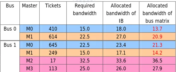
With independent buses architecture, modified traffic model, and bandwidth requirements (shown in Table 4, and same bandwidth requirements are used for independent buses architecture and bus matrix architecture.), local-bus weight tuning can result a ticket assignment (shown in column3 of Table 5) after simulation. All masters meet their bandwidth requirements with the ticket assignment for independent buses architecture (shown in column5 of Table 5). We then check whether the ticket assignment is a proper

ticket assignment or not for bus matrix architecture. The bandwidth allocation for each master is shown in column6 of Table 5 after bus matrix architecture is simulated with the ticket assignment resulted from independent buses architecture. As shown in Table 5, the ticket assignment resulted from independent buses is not a proper ticket assignment for bus matrix architecture because some of bandwidth requirements are not met (shown in column6 of Table 5). In other words, independent buses architecture fails to model behavior of bus matrix architecture.

Table 4 : The bandwidth requirement of Figure 15 and Figure 16 Bus Master Required bandwidth

M0 15 Bus 0 M1 22.5 M0 22.5 M1 15 M2 32.5 Bus 1 M3 25

Table 5 : The simulation result of Figure 15 and Figure 16

Bus Master Tickets Required bandwidth Allocated bandwidth of IB Allocated bandwidth of bus matrix M0 410 15.0 18.0 13.7 Bus 0 M1 614 22.5 27.0 20.9 M0 645 22.5 23.4 21.3 M1 249 15.0 17.1 14.2 M2 17 32.5 33.6 36.5 Bus 1 M3 113 25.0 26.0 27.9

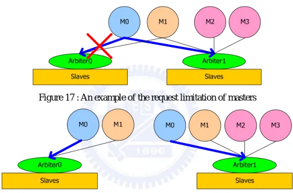
request is not completed, M0 can not initiate any new request. The traffic behavior on different bus is not independent to each other on the bus matrix architecture. As shown in Figure 18, if M0 had initiated a request on bus 1, M0 can initiate another request on bus 0. Traffic behavior of bus matrix architecture and independent buses architecture is totally different. In other words, it is no suitably that using independent buses architecture models behavior of bus matrix architecture.

Figure 17 : An example of the request limitation of masters

Figure 18 : An example shows the difference between IB and Figure 17

2.4.2 Bus matrix architecture with local-bus weight tuning

In fact, bus matrix architecture can use local-bus weight tuning directly. Local-bus weight tuning algorithm deals with ticket redistribution on only one bus at one time. Local-bus weight tuning algorithm takes information of only one bus into consider first, and then it redistributes tickets of masters on the bus. After it completes ticket redistribution on previous bus, local-bus weight tuning considers information of another bus and redistributes tickets of masters on that bus. Local-bus weight tuning algorithm

redistributes tickets bus by bus. In Figure 19, for example, there are two buses, bus 0 and bus 1. Bus 0 consists of M0, M1, M2, and M3, and Bus 1 consists of M0, M1, M4, and M5. Assume Mleast of bus 0 is M1 and Mleast of bus 1 is M0 (section2.3). Local-bus weight

tuning algorithm takes information of bus 0 into consideration at first. According to information of bus 0, local-bus weight tuning algorithm increases tickets to M1 on the bus 0. After redistributing tickets on the bus 0, then local-bus weight tuning algorithm take information of bus 1 into consideration. According to information of bus 1, local-bus weight tuning algorithm increases tickets to M0 on the bus 1.

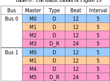
With bus matrix architecture shown in Figure 19 and respective traffic model shown in Table 6, local-bus weight tuning can result a ticket assignment for bus matrix architecture after simulation. Resultant ticket assignment and allocated bandwidth of masters are shown in Table 7. As shown in Table 7, each bus has total 1024 tickets. M1 on the bus 0 has more than 50% tickets of total tickets of bus 0, but it does not meet its bandwidth requirement; M0 on the bus 1 has more than 50% tickets of total tickets of bus 1, but it does not meet its bandwidth requirement either.

M0 Arbiter0 Slaves Arbiter1 Slaves r40% r60% M1 r40% r60% M4 M5 M2 M3

Table 6 : The traffic model of Figure 19 Bus Master Type Beat Interval

M0 D 12 5 M1 D 12 5 M2 D 12 5 Bus 0 M3 D_R 24 5 M0 D 12 5 M1 D 12 5 M4 D 12 5 Bus 1 M5 D_R 24 5

Table 7 : The simulation result of Figure 19 with the local-bus weight tuning Bus Master Tickets Required

bandwidth Allocated bandwidth of bus matrix M0 220 15.0 13.8 M1 554 21.0 19.9 M2 198 34.9 37.5 Bus 0 M3 52 19.1 28.8 M0 624 22.5 21.0 M1 156 14.0 13.3 M4 186 33.6 37.3 Bus 1 M5 58 19.9 28.4

In this example, we observe that the bandwidth allocation of a MM on each bus has a fixed proportion. For example, M0 is a MM connecting with bus 0 and bus 1 in Figure 20. When M0 initiates a request, the request has 20% probabilities to bus 0 and 80% probabilities to bus 1. The request ratio of M0 is 1:4. Assume the beat number of M0 on bus 0 is as same as on bus 1. We observe that if M0 gets 1% bandwidth on bus 0, M0 gets about 4% bandwidth on bus 1. If M0 gets 8% bandwidth on bus 1, M0 gets about 2% bandwidth on bus 0. The ratio of bandwidth allocation on bus 0 to bandwidth allocation on

bus 1 is 1:4. The bandwidth allocation of an MM is proportional to the request ratio if the beat numbers of the MM on all connecting buses are the same. In other words, the bandwidth allocation is related to the request ratio.

Figure 20 : An example of a MM with the request ratio equaling to 1:4

The relationship between bandwidth allocation and request ratio implies that if an MM misses one bandwidth requirement on one bus, the MM misses all bandwidth requirements on other buses which connect to the MM. As shown in Figure 21, the bandwidth requirement of M0 on bus 0 is 4%, and the bandwidth requirement of M0 on bus 0 is 16%. Assume the beat number of M0 on bus 0 is as same as on bus 1, and the request ratio of M0 is 1:4. If M0 gets 2% bandwidth on the bus 0 which is 2% less than the bandwidth requirement, and then M0 gets 8% bandwidth on the bus 1 which is 8%less than the bandwidth requirement. If M0 gets 4% bandwidth on the bus 1 which is 12% less than the bandwidth requirement, and then M0 gets 1% bandwidth on the bus 0 which is 3% less than the bandwidth requirement. Only if M0 gets 4% bandwidth on the bus 0 or 16% bandwidth on the bus 1, M0 can meet all bandwidth requirements on different buses.

M0 Arbiter0 Slaves Arbiter1 Slaves r20% _r80% 16 4 3 1 2 2 8 8 12 4 Requirement is 4 Requirement is 16

Figure 21 : An MM misses or meets all bandwidth requirements

The relationship between bandwidth allocation and request ratio implies another thing. Figure 22 is as same as Table 7. As shown in Figure 22, M0 on the bus 0 holds too fewer tickets and misses it bandwidth requirement. It induce that M0 misses its bandwidth requirement on bus 1. An MM misses its bandwidth requirement on a bus because it does not hold enough tickets to meet the bandwidth requirement on other buses.

When the local-bus weight tuning algorithm tunes the tickets of masters, it only considers with the information of one bus at one time and every bus tunes its tickets individually. If a master misses its bandwidth requirement on a bus, the local-bus weight tuning algorithm thought that the master needs more tickets and increase its tickets on this bus. But, an MM may miss its bandwidth requirement on a bus because it does not hold enough tickets to meet the bandwidth requirement on other buses. If an MM does not hold enough tickets to meet the bandwidth requirement on one bus, all bandwidth requirements

of other buses miss. The local bus weight tuning algorithm may not be a suitable weight tuning algorithm for bus matrix because it does not take the dependence between each bus into consideration.

Tickets Required bandwidth

(%) Allocated bandwidth of multi-bus (%) M0 220 15.0 13.8 M1 554 21.0 19.9 M2 198 34.9 37.5 M3 52 19.1 28.8 M0 624 22.5 21.0 M1 156 14.0 13.3 M4 186 33.6 37.3 M5 58 19.9 28.4

Bus0

Bus1

Figure 22 : A missed bandwidth requirement on a bus induces all bandwidth missed on other buses

According to our observation, the weight tuning algorithm cannot only consider with the information of only one bus at one time for the bus matrix architecture. For bus matrix architecture, the weight tuning algorithm has to take more information from different buses into consideration. We propose a new weight tuning algorithm which is more suitable for bus matrix architecture.

Chapter 3

The proposed Algorithm

3.1 A weight tuning algorithm with multi-bus consideration

When the local-bus weight tuning algorithm redistributes tickets for masters, it take information of only one bus into consideration at one time. Because of the limitation, we propose a weight tuning algorithm with multi-bus consideration, called MC weight tuning briefly. The MC weight tuning takes advantages of the local-bus weight tuning algorithm, which has precise controllability over the bandwidth allocation for SMs. In addition, the MC weight tuning algorithm takes information of more than one bus into consideration. MC weight tuning algorithm can redistributes tickets for MMs on many buses at one time.

The flow chart of MC weight tuning algorithm is shown in Figure 23. As shown in Figure 23, there are two loops in the MC weight tuning algorithm. The red number in each block is the block number. The outer loop consists of block2, block8, and block9, and the

inner loop consists of block 3, block 4, block 5, block 6, and block 7. In outer loop, the global-bus weight tuning (block 9) can redistribute tickets of MMs on many buses at one time. The inner loop is the flow of the local-bus weight tuning algorithm, and it can fine tune the ticket assignment resulting from the outer loop. In block 2, there is a ticket assignment resulting from the outer loop, and it is changed when it go into inner loop. The ticket assignment in block 2 is saved in other memory region before it is changed by inner loop because we want to know the ticket assignment before the step going into inner loop. The ticket assignment in block 2 is called intermediate ticket assignment.

As shown in Figure 23, we have a given initial ticket assignment (block 1) at first. Then, the step goes to block 2 to save the ticket assignment before going into inner loop (the saved ticket assignment is called intermediate ticket assignment). After saving the intermediate ticket assignment, the step goes to the flow of local-bus weight tuning (inner loop). In the inner loop, it checks whether the local-bus weight tuning algorithm can meet all bandwidth requirements of masters or not. If it can, the simulation is terminated (block 5) and result the ticket assignment which can meet all bandwidth requirements. If it cannot meet all bandwidth requirements, the step goes to block 8 and check there is any SM missing its bandwidth requirement. Because of the local-bus weight tuning algorithm providing precise controllability over the bandwidth allocation for SMs, if there is any SM missing its bandwidth requirement, the simulation is terminated and result current ticket assignment (block 10). If no SM misses it bandwidth requirement, the step goes to block 9. In other words, if masters which miss their bandwidth requirements all belong to MM, the step goes to block 9. Otherwise, the step goes to block 10 and the simulation is terminated.

their bandwidth requirements on many buses at same time. The details of global-bus weight tuning are introduced later. After tuning tickets of MMs which miss their bandwidth requirements, the step go to block 2 and go on as we described before.

Figure 23 : The flow chart of MC weight tuning algorithm

3.1.1 Notations

We introduce some notations at first in this section before we introduce more detail of MC weight tuning algorithm. There are two special letters for our notations that are “i” and “j”. Letter “i” is used to represent the number of a master. For example, i equals to 1 for M1. Letter “j” is used to represent the number of a bus. For example, j equals to 2 for bus2.

z t : tickets of master i on the bus j. For example, M3 has 257 tickets on bus 1, _{i j,}

3,1 257

t =

z inter t : tickets of master i on the bus j in the intermediate ticket assignment _ _{i j,} (block 2 of Figure 23)

z most : a master which gets the most bandwidth than its bandwidth requirement _j

on the bus j after inner loop terminated. For example, if M3 on bus 1 gets the most bandwidth than its bandwidth requirement after inner loop terminated,

1 M3

most = .

z T most : on the bus j, we decrease tickets from ( _j) most and increase it to the _j

MMs who miss its bandwidth requirement. (T most_j) represents the tickets decreased from most . For example, if M3 on bus 1 gets the most bandwidth _j

than its bandwidth requirement after inner loop terminated, most₁=M3. On the bus 1, we decrease tickets from M3. Assume we decrease 137 tickets from M3 on the bus 1, T most( ₁) 137= .

z Dec most( _j): the coefficient helps us to know how much tickets decrease from

j

most on the bus j. For example, if M3 on bus 1 gets the most bandwidth than

its bandwidth requirement after inner loop terminated, most₁ =M3. Assume M3 has 257 tickets on the bus 1 (t_3,1=257) and the Dec most( ₁)=53% on the bus 1. We decrease 257 53%× =137 tickets from M3 on the bus 1, and then

z less : there can be more than one MM which misses its requirement on the bus j _j

after inner loop terminated. For example, if there are 2 MMs, M1 and M2, on the bus 1 misses their bandwidth requirements after inner loop terminated,

{

}

1 M1, M2 less = .

z T less_k( _j): T less_k( _{i j,} ) represents the tickets increasing to the kth MM of the set j

less . For example, if two MMs, M1 and M2, miss their bandwidth requirements

on bus 1 after inner loop terminated, less₁ =

{

}

z Inc less : the coefficient helps us to know how much tickets increase to the k_k( _j) th

MM of the set less . For example, if M3 on bus 1 gets the most bandwidth than _j

its bandwidth requirement after inner loop terminated, most₁ =M3. And if two MMs, M1 and M2, miss their bandwidth requirement on bus 1 after inner loop finishing, less₁=

{

}

1

( ) 53%

Dec most = , Inc less₁( ₁)=27%, and Inc less₂( ₁)=73% on the bus 1. First, we decrease 257 53% 137× = tickets from M3 on the bus 1 and

1

( ) 137

T most = . Then, we increase

1 1 1 1 1 2 1 ( ) 27% ( ) 137 37 ( ) ( ) 27% 73% Inc less T most

Inc less Inc less

× = × =

+ + tickets to M1 on the bus 1 and increase 1 1

1 1 1 2 1 ( ) 73% ( ) 137 100 ( ) ( ) 27% 73% Inc less T most

Inc less Inc less

× = × =

tickets to M2 on the bus 1. In other words, 1 1 1 1 1 1 1 2 1 ( ) 27% ( ) ( ) 137 37 ( ) ( ) 27% 73% Inc less T less T most

Inc less Inc less

= × = × = + + and 2 1 2 1 1 1 1 2 1 ( ) 73% ( ) ( ) 137 100 ( ) ( ) 27% 73% Inc less T less T most

Inc less Inc less

= × = × =

+ + . Finally,

3,1 257 137 80

t = − = , t_1,1=93 37+ =130, and t_2,1=78 100 178+ = .

z request_ prob : this notation represents the request probability of the master i _{i j,}

on the bus j

z required_bw : this notation represent the bandwidth requirement of master i _{i j,}

on the bus j.

z allocated_bw : this notation represent the bandwidth allocation of master i on _{i j,}

the bus j.

3.1.2 The details of MC weight tuning algorithm

In this section, we illustrate the MC weight tuning algorithm with an example and introduce details of global-bus weight tuning. As shown in Figure 24, there are 2 MMs, M0 and M1, and 4 SMs, M2, M3, M4, and M5 in the bus matrix system. And the traffic model is shown in Table 8. There are In the “Beat” column of Table 8, there are two kinds of beat numbers. For example, if M0 on the bus 0 initiates a request, the beat number is equal to 16 with 50% probabilities and is equal to 8 with 50% probabilities. In the “Interval” column of Table 8, there are five kinds of interval time. For example, if a request of M0 on the bus 0 is completed, the interval time is equal to 3 with 10% probabilities, 4 with 20%

M0 Arbiter0 Slaves Arbiter1 Slaves r40% r60% M1 r40% r60% M4 M5 M2 M3

Figure 24 : The bus matrix system of the example of MC weight tuning Table 8 : The traffic model of Figure 24

Bus Master Type Beat Interval Required

bandwidth (%) 50%/50% 10% 20% 40% 20% 10% M0 D 16 /8 3 4 5 6 7 15.0 M1 D 16 /8 3 4 5 6 7 21.0 M2 D_R 16 /8 3 4 5 6 7 34.9 Bus 0 M3 D 32 /16 3 4 5 6 7 19.1 M0 D 16 /8 3 4 5 6 7 22.5 M1 D 16 /8 3 4 5 6 7 14.0 M4 D_R 16 /8 3 4 5 6 7 33.6 Bus 1 M5 D 32 /16 3 4 5 6 7 19.9

The initial ticket assignment is shown in the third column of Table 9 (block 1). Then the ticket assignment is saved as intermediate ticket assignment (block 2). For example, we set inter t_ _0,0 to 167 (the intermediate tickets of M0 on the bus 0 is 167), inter t to _ _1,0 223 (the intermediate tickets of M1 on the bus 0 is 167), etc.

After saving the ticket assignment to intermediate ticket assignment, the inner loop start and try to meet all bandwidth requirements of masters (block 3, block 4, block 5, block 6, and block 7). When the inner loop terminated, the resultant ticket assignment and bandwidth allocation of each master are shown in the “Tuned tickets” column and the “Allocated bandwidth of bus matrix” column respectively in Table 9. As shown in Table 9, M0 and M1 miss their bandwidth requirements on the bus 0 and bus 1. There is no SM

misses its requirement (block 8). The global-bus weight tuning restores the intermediate ticket assignment first, and then increase tickets to MMs which miss their bandwidth requirements (block 9).

Table 9 : The ticket assignment and bandwidth allocation after inner loop terminated Bus Master Initial

tickets Tuned tickets Required bandwidth (%) Allocated bandwidth of bus matrix M0 167 220 15.0 13.8 M1 257 554 21.0 19.9 M2 387 198 34.9 37.5 Bus 0 M3 213 52 19.1 28.8 M0 274 624 22.5 21.0 M1 156 156 14.0 13.3 M4 373 186 33.6 37.3 Bus 1 M5 221 58 19.9 28.4

The detailed flow of global-bus weight tuning is shown in Figure 25. As shown in Figure 25, the global-bus weight tuning has three steps. First, we restore intermediate ticket assignment and find the most on each bus. Second, tickets are decreased from the _j

j

most on each bus. Finally, we increase tickets to MMs which miss their bandwidth

requirements.

In Table 10, the “More or less than requirement” column is used to find the most on _j

each bus. The “Bandwidth difference” column in Table 10 shows that the difference between allocated bandwidth and required bandwidth of each master. As shown in Table 10, M3 gets the most bandwidth than its requirement on bus 0, so most₀ =M3. And M5 gets

j

most

Figure 25 : The flow of global-bus weight tuning Table 10 : Table 9 with more information

Bus Master Request probability Intermediate tickets Required bandwidth (%) Allocated bandwidth Bandwidth difference (%) M0 r40% 167 15.0 13.8 - 7.9 M1 r60% 257 21.0 19.9 - 5.0 M2 r100% 387 34.9 37.5 7.4 Bus 0 M3 r100% 213 19.1 28.8 50.4 M0 r40% 274 22.5 21.0 - 6.7 M1 r60% 156 14.0 13.3 - 4.4 M4 r100% 373 33.6 37.3 11.0 Bus 1 M5 r100% 221 19.9 28.4 42.7

Tickets are decreased from most at second step of global-bus weight tuning. The _j

decreasing coefficient is calculated first (finding Dec most( _j)). Then we can know how many tickets are decreased from most (finding (_j T most_j)) . Finally, we decrease

( _j)

, , , , ( _ _ ) _ ( ) _ i j i j i j j i j

allocated bw required bw request prob Dec most required bw B − = i (3.1) , ( _j) _ _{i j} ( _j)

T most =inert t iDec most (3.2)

, ,

_ _{i j} _ _{i j} ( _j)

inert t =inert t −T most (3.3) The coefficient “B” is used to avoid the algorithm never stop. When the algorithm goes through the global-bus weight tuning, “B” is increased and Dec most( _j) becomes smaller as “B” increased. When Dec most( _j) equal to zero, the simulation is terminated.

In Table 10, for example, M3 gets the most bandwidth than its requirement on the bus 0 and M5 gets the most bandwidth than its requirement on the bus 1. most₀ =M3 and

1 M5

most = . On bus 0, by the

Equation3.1 3,0 3,0 3,0 0 3,0 100% 5 ( _ _ ) _ ( ) .4 _ 0 %

allocated bw required bw request prob Dec most

required bw B × B

−

= i = . By

the Equation3.2, T most( ₀) inert t_ _3,0 Dec mo( ₀) 213 50.4% 100% 107

B st = × × = = i . On bus 1, by the Equation3.1 5,1 5,1 5,1 1 5,1 100% 4 ( _ _ ) _ ( ) .7 _ 2 %

allocated bw required bw request prob Dec most

required bw B × B

−

= i = . By

the Equation3.2, T most( ₁) inert t_ _5,1 Dec mos( ₁) 221 42.7% 100% 94

B

t = × × =

= i .

At final step of global-bus weight tuning, tickets are increased to MMs which miss their bandwidth requirements after we decreased tickets from most on each bus. The _j

shows how to increase tickets to MMs of less . The following equations show above _j processes. , , , , ( _ _ ) 1 ( ) _ _ i j i j k j i j i j required bw allocated bw Inc less

required bw request prob

− = i (3.4) , , ( ) _ _ ( ) ( ) k j i j i j j k j k Inc less inter t inter t T most

Inc less

= +

∑

i (3,5) In Table 10, for example, less0 =

{

}

0 100% 213 50.4 ( ) % 107 T most B

= × × = tickets from M3 on bus 0. By the Equation3.4,

0,0 0,0 1 0 0,0 0,0 ( _ _ ) 1 1 ( ) 7.9% _ _ 40% required bw allocated bw Inc less

required bw request pro

− = i = × and 1,0 1,0 2 0 1,0 1,0 ( _ _ ) 1 1 ( ) 5% _ _ 60% required bw allocated bw Inc less

required bw request prob

− = i = × . There are 1 0 0 1 0 2 0 7.9% ( ) _40% ( ) 75 7.9% 5% ( ) ( ) 4 10 % 7 0% 60 Inc less T most

Inc less +Inc less = × ₊ =

i tickets are increased to intermediate tickets of M0 on the bus 0 ( inter t_ _0,0 ). There are

2 0 0 1 0 2 0 5% ( ) _60% ( ) 32 7.9% 5% ( ) ( ) 40% 60% 107 Inc less T most

Inc less +Inc less = × ₊ =

i tickets are increased to intermediate tickets of M1 on the bus 0 (inter t ). _ _1,0

On bus 1, less₁ =

{

}

B

t = × × =

tickets from most₁ . By the Equation3.4,

0,1 0,1 1 1 0,1 0,1 ( _ _ ) 1 1 ( ) 6.7% _ _ 60% required bw allocated bw Inc less

required bw request prob

−

1,1 1,1 1 1 1,1 1,1 ( _ _ ) 1 1 ( ) 4.4% _ _ 40% required bw allocated bw Inc less

required bw request prob

− = i = × . There are 1 1 1 1 1 2 1 6.7% ( ) _60% ( ) 47 6.7% 4.4% ( ) ( ) 60% 40% 94 Inc less T most

Inc less +Inc less = × ₊ =

i tickets are increased to intermediate tickets of M0 on the bus 1 ( inter t_ _0,1 ). There are

2 1 1 1 1 2 1 6.7% ( ) _60% ( ) 47 6.7% 4.4% ( ) ( ) 60% 40% 94 Inc less T most

Inc less +Inc less = × ₊ =

i tickets are increased to intermediate tickets of M1 on the bus 1 (inter t ). _ _1,1

After global-bus weight tuning finishes (block 9), the step goes to block 2 and repeats the flow. When the simulation is terminated, it results a proper ticket assignment to masters. In Table 11, the “Final tickets” column shows the proper ticket assignment resulted by MC weight tuning algorithm and it meets all bandwidth requirements of masters. As the result, the MC weight tuning is more suitable for the bus matrix architecture.

Table 11: The simulation result of example Figure 24 by MC weight tuning algorithm Bus Master Initial

tickets Final tickets Required bandwidth Allocated bandwidth M0 167 409 15.0 14.8 M1 257 386 21.0 22.0 M2 387 193 34.9 38.4 Bus 0 M3 213 12 19.1 24.8 M0 274 411 22.5 22.2 M1 156 390 14.0 14.3 M4 373 186 33.6 37.9 Bus 1 M5 221 13 19.9 25.5

Chapter 4

Experimental Results

4.1 Experiment setup

We use the SoC Designer which is developed by ARM to implement our experiments [25]. As shown in Figure 26, there are 2N masters and slaves. Every arbiter with slaves can be regarded as a bus system. Each master can be connected to one or more than one bus systems. Every master has a decoder to transport the request to its destination bus. After a master initiates a request, it puts the request into the respective channel and waits for the response from the corresponding slave. The arbiter selects only one pending request to be granted. The lottery-based arbitration algorithms are used in our experiments. The arbiter forwards the granted request to the corresponding slave and slave responds to the request. After the slave responds, the arbiter puts the response into channel and the master picks up the corresponding response up and completes the transaction.

Arbiter1 Slaves channel channel channel .. . .. . M11 Decoder Request Rsponse M12 De code r M1N De coder Arbiter2 Slaves channel channel channel .. . .. . M21 Decoder M22 De coder M2N De coder

Figure 26 : An example of implementation of a bus matrix system on SoC Designer

4.2 Experiment 1

In experiment 1, we compare the performance with different weight tuning algorithms, local-bus weight tuning algorithm and MC weight tuning algorithm. As shown in Figure 27, there are 4 MMs, M0, M1, M2, and M3, and each bus has 2 SMs (M4, M5, M6, M7, M8, M9, M10, and M11) in the experiment 1. The traffic model on each bus is shown in

is D_R type on the bus 0, but M3 is D type on the bus 1. The beat number of M3 is 8 or 4 on the bus 0, but the beat number of M3 is 16 or 8 on the bus 1. Lottery-based arbitration algorithms are used in experiment 1. The local-bus weight tuning algorithm works on bus matrix architecture and independent buses architecture which is introduced in section 2.4.1. The MC weight tuning algorithm works on bus matrix architecture.

Table 12 : The traffic model of Figure 27

Bus Master Type Beat Interval

50%/50% 10% 20% 40% 20% 10% M0 D 32 /16 3 4 5 6 7 M1 D 16 /8 3 4 5 6 7 M2 D 16 /8 3 4 5 6 7 M3 D_R 8 /4 5 6 7 8 9 M4 D_R 16 /8 3 4 5 6 7 Bus 0 M5 D 32 /16 3 4 5 6 7 M0 D 16 /8 3 4 5 6 7 M1 D 32 /16 3 4 5 6 7 M2 D_R 8 /4 5 6 7 8 9 M3 D 16 /8 3 4 5 6 7 M6 D_R 16 /8 3 4 5 6 7 Bus 1 M7 D 32 /16 3 4 5 6 7 M0 D 16 /8 3 4 5 6 7 M1 D_R 8 /4 5 6 7 8 9 M2 D 16 /8 3 4 5 6 7 M3 D 32 /16 3 4 5 6 7 M8 D_R 16 /8 3 4 5 6 7 Bus 2 M9 D 32 /16 3 4 5 6 7 M0 D_R 8 /4 5 6 7 8 9 M1 D 16 /8 3 4 5 6 7 M2 D 32 /16 3 4 5 6 7 M3 D 16 /8 3 4 5 6 7 M10 D_R 16 /8 3 4 5 6 7 Bus 3 M11 D 32 /16 3 4 5 6 7

We compare the ticket assignments generated by different weight tuning algorithms. If the resultant ticket assignment can make masters meet all real-time requirements and all bandwidth requirements simultaneously, it is a successful case. Otherwise, if one

utilization [16, 24]. We randomly generate pattern for different bus workloads and compare the results. As shown in Table 13, the first column gives the bus workloads varying from 60% to 95%. For example, the “60%~65%” means the workload of each bus is between 60% and 65%. For each set of bus workload, 100 random patterns of different required bandwidth combinations are generated. The “IB & Local” means it simulates on the independent buses architecture with local-bus weight tuning algorithm (introduced in section 2.4.1). The “BM & Local” means it simulates on the bus matrix architecture with local-bus weight tuning algorithm (introduced in section 2.4.2). The “BM & MC” means it simulates on the bus matrix architecture with MC weight tuning algorithm. We accumulate the numbers of success case of three and show them in Table 13.

Table 13 : The number of success case under different weight tuning algorithm Workload (%) IB & Local BM & Local BM & MC

60%~65% 38 90 100 65%~70% 35 86 100 70%~75% 34 80 90 75%~80% 5 53 88 80%~85% 0 38 85 85%~90% 0 0 83

38 35 34 5 0 0 90 86 80 53 38 0 100 100 90 ₈₈ 85 ₈₃ 0 10 20 30 40 50 60 70 80 90 100

IB & Local BM & Local BM & MC

IB & Local 38 35 34 5 0 0 BM & Local 90 86 80 53 38 0 BM & MC 100 100 90 88 85 83

60%~65% 65%~70% 70%~75% 75%~80% 80%~85% 85%~90%

Figure 28 : The figure of Table 13

The independent buses architecture cannot model correctly the behavior of the bus matrix architecture. It has fewer successful cases under different workload. The local-bus weight tuning algorithm using on bus matrix architecture directly can result proper ticket assignment with high successful probabilities below 75% bus workload. Because the local-bus weight tuning algorithm considers information of only one bus at one time, the numbers of successful cases decrease very quickly above 75% bus workload. The MC weight tuning algorithm has 88 successful cases when bus workload is between 75% and 80%. Even bus workload is between 85% and 90% which is extremely high traffic load, the MC weight tuning still has more than 80 successful cases. The MC weight tuning algorithm can result proper ticket assignment for lottery-based arbitration algorithm under

In this experiment, we have the following summaries. The independent buses architecture cannot well model he behavior of the bus matrix architecture. The local-bus weight tuning may work well on the bus matrix architecture when the bus workload is less than 75%. However, the MC weight tuning has better results even if the bus workload is between 85% and 90%.

4.3 Experiment 2

In experiment 2, we compare the performance of MC weight tuning algorithm working on different complexity of bus matrix architecture. As shown in Figure 29, Figure 30, and Figure 31, they all are bus matrix architectures with the different complexities of architectures. There are two buses in Figure 29, three buses in Figure 30, and four buses in Figure 31.

Those three architectures are simulated with lottery-based arbitration algorithms and MC weight tuning algorithm. If the resultant ticket assignment can make masters meet all real-time requirements and all bandwidth requirements simultaneously, it is a successful case. Otherwise, if one requirement is missed, it is a fail case. We randomly generate pattern for different bus workloads and compare the results. As shown in Table 14, the first column gives the bus workloads varying from 60% to 95%. For each set of bus workload, 100 random patterns of different required bandwidth combinations are generated. The “2-bus” means the architecture shown in Figure 29 is used. The “3-bus” means the architecture shown in Figure 30 is used. The “4-bus” means the architecture shown in Figure 31 is used. We accumulate the numbers of successful cases of these three and show the results in Table 14.

Figure 29 : Bus matrix architecture with two buses

Figure 31 : Bus matrix architecture with four buses

Table 14 : The number of success case under different complexity of architectures 2-bus 3-bus 4-bus

60%~65% 100 100 100 65%~70% 100 100 100 70%~75% 100 100 90 75%~80% 98 97 88 80%~85% 98 93 85 85%~90% 92 90 83

0 10 20 30 40 50 60 70 80 90 100

2-bus 3-bus 4-bus

2-bus 100 100 100 98 98 92 3-bus 100 100 100 97 93 90 4-bus 100 100 90 88 85 83

60%~65% 65%~70% 70%~75% 75%~80% 80%~85% 85%~90%

Figure 32 : The figure of Table 14

As shown in Figure 32, the “2-bus” (shown in Figure 29) has the best performance and it is the simplest architecture of those three. The performance of “3-bus” (shown in Figure 30) is very close to that of “2-bus”. Although the performance of “4-bus” (shown in Figure 31) is the worst of the three, the difference of results between “2-bus” and “4-bus” is small. The MC weight tuning algorithm working on different architecture complexity results proper ticket assignment with very high successful rates.

Chapter 5

Conclusions and Future Work

5.1 Conclusions

A new weight tuning algorithm, MC weight tuning algorithm, is proposed in this thesis. It can mostly provide proper ticket assignment to lottery-based arbitration algorithms to meet real-time and bandwidth requirements simultaneously. The MC weight tuning algorithm also shows that the weight tuning algorithm cannot consider information of only one bus at one time. The weight tuning algorithm has to consider information of multiple buses. The experimental results show that the MC weight tuning algorithm working on the bus matrix architecture is better than the local-bus weight tuning algorithm working on the bus matrix architecture. Hence, the MC weight tuning is a better choice for lottery-base arbitration algorithms working on the bus matrix architecture.

As the demands of on-chip communication grow, more modern communication architectures will be proposed in the near future. If lottery-based arbitration algorithms are continually used, an efficient weight tuning algorithm is still needed as well. In the future, we intend to find a weight tuning algorithm which can be used for different communication architectures, even for different weighted or probabilistic arbitration algorithms.