應用已實現波動度於選擇權評價的實證研究

國

立

交

通

大

學

財 務 金 融 所

碩

士

論

文

應用已實現波動度於選擇權評價的實證研究

An Empirical Investigation of Option Pricing Models

with Realized Volatility

研 究 生：邱婉茜

指導教授：周幼珍 博士

應用已實現波動度於選擇權評價的實證研究

An Empirical Investigation of Option Pricing Models

with Realized Volatility

研 究 生：邱婉茜 Student：Wan-Chien Chiu

指導教授：周幼珍 博士 Advisor：Yow-Jen Jou

國立交通大學

財務金融研究所碩士班

碩士論文

A Thesis

Submitted to Graduate Institute of Finance

National Chiao Tung University

in partial Fulfillment of the Requirements

for the Degree of

Master of Science

in

Finance

June 2008

Hsinchu, Taiwan, Republic of China

應用已實現波動度於選擇權評價的實證研究

研究生：邱婉茜 指導教授：周幼珍 博士

國立交通大學財務金融研究所碩士班

2008 年 6 月

摘要

先前文獻已提出：利用高頻率資料的異質性自我相關已實現波動度(HAR-RV)模

型，較其他波動度模型更能捕捉財務市場報酬波動度的特性及更準確的預測波動度。然

而，就本文所知，直到目前為止尚未有研究探討應用 HAR-RV 模型於選擇權中，是否可

減少選擇權評價誤差及增進選擇權 delta 動態避險績效。此外，過去的實證結果發現

EGARCH 模型在選擇權評價上優於其他波動度模型。

因此，本文研究目的為：將 HAR-RV 與 EGARCH 選擇權評價模型用於 S&P500 指

數選擇權的評價，並比較二模型在評價及避險績效上的差異。本文實證結果發現：第一、

除了樣本外的價外買權和價外賣權，HAR-RV 模型在樣本外的買權和賣權的評價誤差較

EGARCH 模型小；第二、HAR-RV 模型在樣本外的買權避險績效較佳，而 EGARCH 模

型在樣本外的賣權避險績效表現較好，然而，此樣本外的賣權避險績效並沒有顯著地比

HAR-RV 模型的樣本外賣權避險績效佳。

關鍵字：高頻率資料、異質性自我相關已實現波動度(HAR-RV)模型、EGARCH 模型、

評價誤差、避險績效。

An Empirical Investigation of Option Pricing Models with Realized Volatility

Student : Wan-Chien Chiu Advisor : Dr. Yow-Jen Jou

Institute of Finance

National Chiao Tung University

ABSTRACT

Previous studies have documented that, with use of high frequency data, Heterogeneous Autoregressive of the Realized Volatility (HAR-RV) model performs better than other volatility models in fitting financial return volatility measurement and has a more accurate forecasting ability. However, to our knowledge, no previous studies have investigated whether the HAR-RV model can improve option pricing and delta dynamic hedging performance in financial markets. Additionally, previous empirical analysis of option pricing models with the framework of EGARCH have presented superior to other volatility models. Using S&P 500 index options data, this study compares the HAR-RV and the EGARCH option pricing model in terms of option pricing and dynamic hedging performance. As expected, the results of this study demonstrate that the HAR-RV option pricing model is superior in terms of out-of-sample call and out-of-sample put option pricing performance for all moneyness except for out-of-the-money options. In out-of-sample hedging performance, the HAR-RV model still performs better than the EGARCH model, except in the case of put options. However, the EGARCH option pricing model does not show significant superiority in hedging performance of put options.

Keywords: High frequency data; HAR-RV option pricing model; EGARCH option pricing model;

誌 謝

本論文能夠順利完成首先誠摯地感謝指導教授周幼珍老師，接受老師指導的這段

期間，謝謝老師能包容我的想法，並適時地引導正確論文方向，以及在我需要幫助的

時候,給予我最大的支持。同時也要感謝口試委員鍾惠民老師、韓傳祥老師、孫而音

老師，對本論文提供許多寶貴的建議，以及寶來金融集團的讚助，不勝感激。

再來我要感謝在交大財金所陪伴我的同學們，其中我的同學兼好朋友－育維，在

這兩年帶給我的歡樂，讓我忘記研究的苦悶，快樂的過每一天。還有志瑋，感謝你這

兩年陪我一起學習、一起成長，和你一起共同討論，才有這篇論文產生，在研究遇到

瓶頸的時候，謝謝你包容我的壞脾氣，有你的鼓勵我才有繼續完成論文的動力，非常

開心能有你的這個好同學好朋友。

最後，感謝我的家人們，一直以來很相信我、支持我的決定，當我在新竹唸書到

很累的時候，回到家吃到媽媽做的飯，在家裡睡一晚的覺，就又有精神繼續學習了；

最後要感謝的是我的父親，辛勞的工作養育我之外，亦常常關心我的生活，讓我感到

很窩心。謝謝你們才成就現在的我。

婉茜 戍子年夏天

僅誌於 新竹交大

Content

Chinese Abstract……….i

English Abstract……….ii

Chinese Acknowledgements………..iii

Content………..iv

List of Tables………..v

List of Figures………...vi

1. Introduction……….1

2. Data……….3

3. Volatility Models……….4

3.1. EGARCH model……….4

3.2. HAR－RV model………5

4. European Option Pricing Models………...7

4.1 The EGARCH option pricing model………...7

4.2 The HAR-RV option pricing model………8

5. Out-of-Sample Pricing Performance……….11

5.1 One-Day Out-Of-Sample Pricing Performance………..12

5.2 Five-Days Out-Of-Sample Pricing Performance………12

6. Out-of-Sample Dynamic Delta Hedging Performance………..12

6.1. The Mechanism of Dynamic Delta Hedging……….12

6.2. Out-of-Sample Dynamic Delta Hedging Performance………..14

List of Tables

Table 2.1 Summary Statistics of SPX in Call Options………...18

Table 2.2 Summary Statistics of SPX in Put Options………18

Table 4.1 Summary Statistic of the Parameter Estimators of the EGARCH Option

Pricing Model……… 19

Table 4.2 Summary Statistic of the Parameter Estimators of the HAR-RV Option

Pricing Model……….19

Table 5.1 One-day Out-of-sample Valuation Error for Call Options………..20

Table 5.2 One-day Out-of-sample Valuation Error for Put Options………21

Table 5.3 Fives-day Out-of-sample Valuation Error for Call Options……….22

Table 5.4 Fives-day Out-of-sample Valuation Error for Put Options………..23

Table 6.1 Dynamic Delta Hedging Errors for SPX Call Options………24

List of Figures

Figure 5.1 One-day forecasting errors for SPX Call Options………26

Figure 5.2 One-day forecasting errors for SPX Put Options……….27

Figure 5.3 Five-days forecasting errors for SPX Call Options……….28

Figure 5.4 Five-days forecasting errors for SPX Put Options………...29

Figure 6.1 Dynamic Delta Hedging Errors for SPX Call Options………30

1. Introduction

Since Black and Scholes (1973) introduced their renowned framework for option pricing, numerous theoretical and empirical studies have investigated option pricing. Many empirical studies found that the Black-Scholes model (henceforth BS) includes pricing errors across different situations of moneyness and maturity. In relation to identifying problems on the BS model, people have widely criticized the underlying assumptions of the model. An essential assumption of the BS model is that the underlying asset process follows the log normality distribution with constant volatility. However, the log normality cannot explain various empirical discoveries involving asset return series, most notably the characteristics of fat-tail and volatility clustering. Therefore, various attempts have been made to relax the assumptions of “constant volatility” in BS model.

In the framework of generalized autoregressive conditional heteroskedasticity (GARCH) model introduced by Bollerslev (1986), volatility is allowed to depend on past innovations and volatilities, and thus the model can, in principle, interpret both excess kurtosis and volatility clustering. The model has been successfully applied to financial data such as stock return data, as demonstrated in the survey of Bollerslev et al. Various extended studies have adjusted original GARCH models to better fit real stock returns. In particular, Nelson (1991) identified the phenomenon of asymmetric volatility responses to negative and positive changes in returns, called exponential GARCH (EGARCH) model. It can explain the phenomenon known as the leverage effect, which refers to the tendency for changes in stock price to be negatively correlated with volatility. To date, numerous studies have demonstrated that EGARCH outperforms GARCH in volatility forecasting.

Recently, researchers have found it more effective to use high frequency data for analysis. Anderson, Bollerslev, Diebold and Labys (2001) (henceforth ABDL) proposed a non-parametric method of volatility measurement that used intraday asset return data. The volatility model introduced by ABDL is termed “realized volatility”, and involves the summation of square intraday asset return. ABD and other authors further established the applicability of modeling and forecasting RV in a series of papers (ABDL (2003) and ABD (2005)).

The Heteroskedasticity AR (HAR) model proposed by Corsi (2003) is called HAR-RV model, and is based on the concept that realized volatility is parameterized as a linear function of the lagged realized volatilities over different horizons. Although the HAR-RV model does not formally possess

long-memory, the mixture of relatively few volatility components makes it capable of reproducing remarkable slow volatility autocorrelation decay. The simulation results in Corsi (2003) seem to confirm that the HAR-RV model successfully fits the main empirical features of financial data (long memory and fat tail) in a simple and parsimonious way. Furthermore, the author found that the HAR-RV model outperforms ARFIMA in terms of volatility forecasting ability. Extension of the HAR-RV model to the HAR-RV-CJ model by ABDL (2007) is based on the mathematical results proposed by Barndorff-Nielsen et al. (2004). ABDL (2007) considered realized volatility a combination of integrated volatility and jump component. The authors found that integrated volatility is more persistent than jump, and that jump lacks any forecasting ability.

In the application of option pricing, numerous empirical studies have discussed the use of non-constant volatility in option models. Hull and White (1987) and Heston (1993) introduced a continuous-time stochastic volatility model. Additionally, Duan (1995) developed an option pricing model based on the GARCH process. Moreover, Bakshi, Cao, & Chen (1997)(henceforth BCC) assessed the performance of various models allowing volatility, interest rates, and jumps to be stochastic for S&P500 index option contracts. BCC found that although the BS model does not outperform other more complicated models in terms of either in-sample fitting or out-of-sample forecasting, it does achieve comparable hedging performance. Dumas, Fleming, & Whaley (1998) assessed an ad hoc version of the BS model, and found that it performs no worse than a class of so-called deterministic volatility function models. For hedging purposes, they concluded that “simpler is better.” Heston and Nandi (2000) investigated the empirical performance of alternative option pricing models using S&P500 Index options data and found that GARCH outperforms the ad hoc BS model of Dumas et al. (1998) in terms of in-sample fitting and out-of-sample forecasting. Haynes, Yung, & Zhang (2003) compared the empirical performance of an ad hoc BS option pricing model with that of an EGARCH option pricing model, and found that EGARCH outperforms the ad hoc BS model in terms of both in-sample fitting and out-of-sample forecasting. However, the EGARCH performs worse than the ad hoc BS model in terms of hedging performance regardless of moneyness and hedging horizons.

Previous studies demonstrate that the HAR-RV model is superior to alternative models for volatility forecasting. Furthermore, based on previous studies, EGARCH model has better option pricing performance for both in-sample fitting and out-of-sample forecasting, except in hedging

performance. Although the HAR-RV model is a better volatility model in forecasting, to date, no studies have examined its influence on options pricing. This study thus evaluates pricing performance of S&P 500 index option (SPX) (largely traded European option in U.S.) for two aspects, out-of-sample valuation errors and out-of-sample hedging errors, by using the HAR-RV model and the EGARCH model respectively. This study examines whether the HAR-RV model outperforms the EGARCH model in pricing and hedging performance.

Generally, the results of this study indicate that the HAR-RV option pricing model is superior both in call and put one-day/five-days pricing performance and in call option hedging performance. However, the EGARCH option pricing model does not show significant superiority in put option hedging performance.

The remainder of this paper is organized as follows. Section 2 describes the data, and Section 3 then introduces time series volatility model and realized volatility model. Subsequently, Section 4 describes how SPX can be priced in applying volatilities estimated by HAR-RV model and EGARCH model (see Duan (1995)). Section 5 presents out-of-sample pricing performance, and Section 6 discusses out-of-sample dynamics hedging errors. Conclusions are finally drawn in Section 7, along with recommendations for future research.

2. Data

This work investigates a heavily traded option contract, the S&P 500 index option (SPX). To apply the HAR-RV model, high frequency data are required. Based on the Tickdata database, this study considers the S&P 500 index from Jan. 2, 2002 to June 29, 2007, including daily data and 15 minute interval data. This study used daily data in EGARCH (1,1) models to estimate volatilities, and 15 minute interval data in the HAR-RV model to obtain the estimated volatilities.

Additionally, option data of SPX is necessary to assess pricing performance and hedging errors. This study gathered option data with daily trading volume exceeding five contracts. Although this is not a guarantee against thin trade effects, it should go quite a way in terms of minimizing the problem. Furthermore, the choice of more than five contracts per day is used in the previous literature.

This study takes into account the nearest contract months of option prices with maturity times that are greater than 21 days but less than 90 days. To mitigate the impact of price discreteness on option valuation, options with values smaller than 3/8 are excluded; based on the OptionMetrics

database, options with end of average bid-offer price exceeding 3/8 are included as our sample. In the OptionMetrics database, option data from Apr. 2, 2007 to June 29, 2007, totally 63 trading days, is selected as the sample.

The OptionMetrics database also includes information on zero curve derived from BBA (British Bankers’ Association) LIBOR rates and settlement prices of CME Eurodollar futures. This study extracts necessary data from zero curve as our risk-free interest rates. The zero curve is used for the period from Apr. 2, 2007 to June 29, 2007 for option pricing. The table 2.1 and 2.2 are summary statistics of SPX in call and put options, respectively.

3. Volatility Models

This section introduces our two competing volatility models, which are the EGARCH model and the HAR-RV model, respectively. The results obtained from these two models will be used as the inputs of the pricing models for assessing option pricing performance and hedging errors.

3.1 EGARCH model

The GARCH model fails to explain the leverage effect and is restrictive on parameters. Nelson (1991) found that the volatility responds asymmetrically responses to negative and positive return changes. The model, called exponential GARCH (EGARCH) can explain leverage effect, which refers to the tendency for changes in stock price to be negatively correlated with volatility. Furthermore, numerous studies show that EGARCH performs better than GARCH model in volatility forecasting. The EGARCH (1,1) was proposed by Nelson(1991)as follows.

Define h_t as follows:

(

)

{

0 1 1 1

}

exp t ln t t h = α α+ f z− +β h− f z

( )

_t−1 =

⎡

_⎣

z_t−1 −E Z_t−1 +δz_{t 1−}

⎤

_⎦

(1) where

Z

_t−1 is standard error, defined as

ε

_t−1

h

_t−1 , which conditional on the previous information, are independent random variables with mean zero, and variance one. In addition,

1 1

t t t 1

z

₋

−

E Z

₋

+

δ

z

₋ is an asymmetric formula of

z

_t−1.

Considering this f function,

z

_t−1

−

E Z

_t−1 is a measure of shock size when volatility is systematic, called magnitude effect, and

δ

z

_t−1 represents sign effect, which is a new shock in the

asymmetric formula. The full asymmetric formula represents the current volatility determined by past shock size and sign. Furthermore, the distribution of

Z

t−1 should be set when using MLE. Nelson (1991) use generalized error distribution, whose pdf is as follows:

( )

{

}

{

( )

( )

}

1 1

exp

0.5

2

3

f z

ν

z

λ

ν

λ

ν ν − ⎡ − ⎤ ⎣ ⎦

⎡

⎤

=

⋅

_⎣

−

_⎦

⋅

⋅

⋅Γ

ν

(2)

where

λ

=_⎣⎡2−2ν ⋅Γ

( ) ( )

1

ν

Γ 3

ν

⎤_⎦0.5,

ν

controls the thickness of distribution tail,

Γ ⋅

( )

is a Gamma function, and E Z

(

t−1

)

= 2

π

. Therefore, the EGARCH (1,1) model for the random variable rcan be represented as follows:

=

+

t t

r

μ ε

_t

(

)

1 0, t t N ht

ε

Ω ∼₋

(

)

{

0 1 1 1 1 1 1

}

exp 2 ln t t t t t h =

α α ε

+ ⋅_⎣⎡ ₋ h₋ −

π δ ε

+ ₋ h_{− ⎦}⎤+

β

ht₋ (3) 3.2 HAR-RV model

The Heterogeneous Autoregressive model of the Realized Volatility (HAR-RV) is proposed by Corsi (2003), which can directly model and forecast the time series behavior of volatility. The model is based on a straightforward extension of the so-called Heterogeneous ARCH, or HARCH, class of models analyzed by Müller et al. (1997). The purpose of the model is to obtain a conditional volatility model based on realized volatility which is able to reproduce the memory persistence observed in the data but, at the same time, remains parsimonious and easy to estimate. The simulation results in Corsi (2003) seem to confirm that the HAR-RV model successfully fits the main empirical features of financial data (long memory and fat tail) in a simple and parsimonious way. Furthermore, empirical results on USD/CHD data by applying HAR-RV model represent good out of sample forecasting performance which steadily and substantially outperforms other previous model (standard GARCH and SV models) (see Corsi (2003)). The following introduces the main framework of HAR-RV model in Corsi (2003):

Assuming that the logarithmic asset price follows a continuous-time process:

dp t

( )

=

μ

( )

t dt

+

σ

( )

t dW t

( )

(4)

where

p t

( )

is the logarithm of instantaneous price,

μ

( )

t

is a continuous, finite variation process,

dW t

( )

is the standard Brownian motion, and

σ

( )

t

is a stochastic process independent

of . For this diffusion process, the integrated volatility associated with day

t

, is the integral of the instantaneous volatility over the one day interval

( )

dW t

(

t

−

1 ;

d t

)

, where a full 24 hours day is represented by the time interval

1d

,

( )

(

( )

)

1 2 2 1 t d t t d

d

σ

σ ω

−

=

∫

ω

(5)

Andersen et al. (2001), applying the quadratic variation theory, suggested that the sum of intraday squared returns converges (as the maximal length of returns go to zero) to the integrated volatility of the prices. This nonparametric estimator is called realized volatility. The definition of the realized volatility over a time interval of one day is

( ) 1 2 0 M d t j t j

RV

−

r

_{− Δ} =

=

∑

(6) where 1d M

Δ = and

r

_{t j− Δ}

=

p t

(

− Δ −

j

)

p t

(

− + Δ

(

j

1

)

)

defines continuously compounded -frequency returns. Under these assumptions, the ex-post realized volatility is an unbiased volatility estimator. Moreover, as the sampling frequency is increased, the realized volatility provides a consistent nonparametric measure of the integrated volatility over the fixed time interval:

Δ

( ) ( )

lim

_{M t}d _td

p

_→∞

RV

=

σ

.

When considering realized volatility over different time horizons longer than one day, these multi-period volatilities are normalized sums of the one-period realized volatilities (i.e. a simple average of the daily quantities). For example, a weekly realized volatility and a monthly realized volatility at time will be given by the average as follows respectively:

t

( ) 1

(

( )₁ ( )₂ ( )₃ ( )₄ ( )

)

5 W d d d d t t d t d t d t d t RV = RV₋ +RV₋ +RV₋ +RV₋ +RV₋d_5d (7) ( ) 1

(

( )₁ ( )₂ ( )₂

)

22 M d d t t d t d RV = RV₋ +RV₋ + +… RV_t−d_2d (8)

Then the one-day ahead volatility is expressed as a linear function of previous realized volatilities, ( ) ( ) ( ) ( ) ( ) ( ) ( ) 1 0 d d d W W M M t d t t t t d

RV

₊

=

β

+

β

RV

+

β

RV

+

β

RV

+

ε

₊₁ ,t=1, 2,…,T (9) The Equation (9) is labeled as a Heterogeneous Autoregressive model for the Realized

Volatility (HAR-RV) model.

4. European Option Pricing Models

In this section, European option pricing model will be combined with the previously described models of volatility to assess the values of SPX.

4.1. The EGARCH option pricing model

For the time varying volatilities estimated from the EGARCH model, there is no analytical solution for pricing options. In this study, we only consider the EGARCH(1,1) model with S&P 500 Index value

S

t is assumed to be the following price dynamics under probability measureP:

2 1 1 ln 2 t t t t S r S₋ = +

λσ

−

σ

+

ε

t

{ }

. . .

( )

0,1

t t t

z

z

t

i i d N

ε σ

=

∼

ln

σ

_t2 = +

ω ϕ σ

ln _t2₋₁+

θ

z_t−1+

γ

_⎣⎡z_t−1 −E z

( )

_t−1 ⎤_⎦ (10)

where

S

_t is the asset price at time ,

t

r is the risk-free rate of return on the asset, and

σ

t2is the conditional variance of the asset at time . Notice that

t

E Z

(

_t−1

)

= 2

π

.

Following Duan (1995), under the locally risk-neutralized measure Q, the stock price process is represented as follows: 2 1 1 ln 2 t t t t S r S₋ = −

σ

+

ξ

(

)

t t t t

z

t t t

z

ξ ε λσ

_{= +}

₌

σ

₊

λ

₌

σ

∗

{ }

z

_t∗ Q

∼

i i d N

. . .

( )

0,1

2 2 1 1 1 2 ln

σ

_t

ω ϕ σ

ln _t

θ

z_t

γ

z_t

π

− − − ⎡ ⎤ = + + + _⎢ − _⎥ ⎣ ⎦

(

)

2 1 1 1 2 ln _t z_t z_t

ω ϕ σ

θ

λ

γ

λ

π

∗ ∗ − − − ⎡ ⎤ = + + − + _⎢ − − _⎥ ⎣ ⎦ (11)

According to the definition of pricing option, the call option price at time with maturity time and strike price

,

_t

,

t C

T X is ( )

{

₍

₎

}

, 0

r T t Q t t T

C

=

e

− −

E

⎡

_⎣

Max

S

−

X

⎤

_⎦

(12) , and the put option price at time

t P

, ,

_t with maturity time T and strike priceX is

( )

{

₍

₎

_{, 0}

}

r T t Q

t t T

P

=

e

− −

E

⎡

_⎣

Max

X

−

S

⎤

_⎦

(13) where E is the expectation operator under measure Q and is the risk-free rate. tQ r

Therefore, there are two steps to implement the EGARCH(1,1) option pricing model. First is to build the EGARCH(1,1) and forecast the one-step-ahead volatility. In this thesis, rolling window approach is used to forecast the volatilities. For example, when pricing the option of April 2, 2007, the daily index data from Jan. 2, 2002 to Mar. 30 2007 are used to build the EGARCH(1,1) model and the predicted volatility of April 2, 2007 are obtained accordingly. The predicted volatility of April 3, 2007 will be obtained using the historical data of the same length by dropping the data of Jan. 2, 2002 and adding that of April 2, 2007. The process goes on as time evolve until June 29, 2007.

The second step of EGARCH option pricing consists of first simulating N (5000 in our case) prices one period ahead according to (11) by Monte Carlo simulation. The simulation process continues in the next period, and so on until option maturity. Finally, the average value of

(

)

{

_T , 0

}

Max S −X and the average value of Max

{

(

X −S_T

)

, 0

}

are discounted to yield the estimated European call and put option value, respectively.

Repeating this procedure, there are total 63 sets of estimated EGARCH(1,1) parameters; at the same time, the option from Apr. 2, 2007 to June 29, 2007 (63 trading days, total 7011 number of options) are evaluated for our interests of out-of-sample option pricing performance. In this study, we called this procedure: “window rolling”. When accounting for one-day out-of-sample valuation error, the data rolls one day every time; for five-days out-of-sample valuation error, it rolls five days every time. Table 4.1 reports the summary statistics of the parameter estimators of the EGARCH(1,1) option pricing model.

4.2. The HAR-RV option pricing model

Since the realized volatility is not a constant volatility, there is no analytic formula to price option. Similar to the EGARCH option pricing model discussed above, in this section, the same Monte Carlo simulation method for option pricing is used. The procedure of the HAR-RV option pricing model is introduced as follows:

Under the risk-neutral world, assuming that the logarithmic asset price follows a continuous-time process:

dp t

( )

=

μ

( )

t dt

+

σ

( )

t dW t

( )

(14)

where

p t

( )

is the logarithm of instantaneous price,

μ

( )

t

is a continuous, finite variation process,

dW t

( )

is the standard Brownian motion, and

σ

( )

t

is a stochastic process independent of

dW t

( )

. By Ito’s lemma, the above equation can be represented as

2

ln

2

t t

d

S

=

⎛

_⎜

r

−

σ

⎞

_⎟

dt

+

σ

dW

⎝

⎠

t t (15)

where

S

_t is the underlying asset price.

When considering discrete time process, the process becomes:

(

)

( )

2

ln

ln

2

t t

S t

+ Δ −

t

S t

=

_⎜

⎛

r

−

σ

⎞

_⎟

Δ +

t

σ ε

Δ

t

⎝

⎠

(16) which is equal to

(

)

( )

exp 2 2 t t S t+ Δ =t S t ⎡_⎢⎜⎛r−

σ

⎞_⎟Δ +t

σ ε

Δt⎤_⎥ ⎝ ⎠ ⎣ ⎦ (17)

where ris risk-free interest rate,

Δ

t

is time interval,

( )

. . .

0,1

i i d

N

ε

∼

Similar to the EGARCH option pricing model, however, the meaning of stochastic variable

t

σ

in this part is realized volatility

RV

_t( )d , defined in HAR-RV model. Based on the notations in

the EGARCH option pricing model, the call option price at time with maturity time and strike price

,

C_t

t

,

T X is ( )

{

₍

₎

}

, 0

r T t Q t t T

C

=

e

− −

E

⎡

_⎣

Max

S

−

X

⎤

_⎦

(18) and the put option price at time is

t

( )

{

₍

₎

}

, 0

r T t Q

t t T

P

=

e

− −

E

⎡

_⎣

Max

X

−

S

⎤

_⎦

(19)

The right-hand side of the above formula is calculated by first simulating (5000, the same as in EGARCH option pricing model) prices one period ahead according to the system in Equation (17) by applying Monte Carlo simulation. Notice that how we determine

N

t

σ

based on HAR-RV

model:

(20) with the high frequency index data from Jan. 2, 2002 to Mar. 30, 2007 (in this paper, per 15 minutes high frequency index data is used).

( ) ( ) ( ) ( ) ( ) ( )

1 0

d d d W W M M

t d t t t t d

RV

₊

=

β

+

β

RV

+

β

RV

+

β

RV

+

ε

₊₁ ,t=1, 2,…,T (20) After that, forecasting ahead one-day volatility by

( )1 ₀ ( ) ( ) ( ) ( ) ( ) d d _d W _W M M t d _{t t t}

RV

+

=

β

+

β

RV

+

β

RV

+

β

RV

(21) where ( ) 1

(

( )₁ ( )₂ ( )₃ ( )₄ ( )₅

)

5 W d d d d t t d t d t d t d t d RV = RV₋ +RV₋ +RV₋ +RV₋ +RV₋d ( )

(

( ) ( ) ( )

)

1 2 2 1 22 M d d t t d t d RV = RV₋ +RV₋ + +… RV₋2 d t d Let ( )1 d t d _t

RV

+

=

σ

and put into

(

)

( )

2 exp 2 t t S t+ Δ =t S t ⎡_⎢⎜⎛r−

σ

⎞_⎟Δ +t

σ ε

Δt⎤_⎥ ⎝ ⎠ ⎣ ⎦ , it will

generate ; then, the simulation process continues in the next period. Similarly, it can generate by the following equation

(

S t

+ Δ

t

)

)

(

2

S t

+ Δ

t

(

)

(

)

12 1 2 exp 2 t t S t+ Δ =t S t+ Δt _⎢⎡_⎜⎛r−

σ

+ _⎟⎞Δ +t

σ ε

₊ Δt_⎥⎤ ⎝ ⎠ ⎣ ⎦ (22) Here, we decide ₁ ( )2 d t d t

RV

σ

₊

=

+ according to the system in Equation (21) by letting

( ) ( ) 1 d d t d t

RV

=

RV

+ , ( ) ( )1 W W t d t

RV

=

RV

+ , ( ) ( )1 M M t d t

RV

=

RV

+ (23) where ( )1 ( )₁ ( )₂ ( )₃ ( )₄ ( )1

1

5

W d d d d d t d _{t d t d t d t d} t d

RV

+

=

⎛

⎜

RV

₋

+

RV

₋

+

RV

₋

+

RV

₋

+

RV

+

⎞

⎟

⎝

⎠

(24) ( )1 ( )₁ ( )₂ ( )₂₁ ( )1

1

22

M _{d d d} d t d _{t d t d t d} t d

RV

+

=

⎜

⎛

RV

₋

+

RV

₋

+ +

RV

₋

+

RV

+

⎞

⎟

⎝

…

⎠

(25)

That is to say, for obtaining the next period one-day forecasting volatility, the main procedure is determine ( )1 and W t d

RV

+ ( ) 1 M t d

RV

+ , which are the average of the past five realized volatilities by both deleting the first historical realized volatility and at the same time, adding a new one-day forecasting realized volatility based on their original set.(see equation (24) and equation (25)). Repeating the procedure until achieving the expiration date (denoted asT ) of options, then we have 5000 numbers of estimated

S T

( )

for evaluating options.

By definition, the average value of Max

{

(

S T

( )

−X

)

, 0

}

and the average of

( )

(

{

)

, 0

}

Max X −S T are discounted to yield the estimated European call and put option value, respectively. Similar to the above part, there are 63 numbers of days option as our sample for evaluating out-of-sample option pricing errors with the HAR-RV model. Table 4.2 reports the summary statistics of the parameter estimators of the HAR-RV option pricing model. Next section, we show our empirical results for SPX.

5. Out-Of-Sample Pricing Performance

We will use three of the most commonly used evaluation criteria in the literature to examine the performance of the option pricing models at two different lengths of pricing period. Let and

denote the observed and the estimated th price, respectively. For

k

P

k

P

k

K observations, the

forecasting criteria are defined as:

1. The mean bias: 1

(

)

1 K k k k MBIAS K− P P = ≡

∑

−

2. The mean absolute error: 1

1 K k k k MAE K− P P = ≡

∑

−

3. The relative mean absolute error: 1 1 K k k k k P P RMAE K P − = − ≡

∑

Additionally, to investigate the moneyness effect of options, based on the scale of

S K

, this study considers six segments:

S K

<

0.94

,

0.94

≤

S K

≤

0.97

,

0.97

≤

S K

≤

1.00

,

1.00

≤

S K

≤

1.03

,

1.03

≤

S K

≤

1.06

, and

S K

>

1.06

. For call option, the option is said to out-of-the-money (OTM) if its

S K

≤

0.97

; at-the-money (ATM) if

S K

∈

(

0.97,1.03

)

; and in-the-money (ITM) if

S K

≥

1.03

.

However, for put option, it is called out-of-the-money (OTM) if its

S K

≥

1.03

; at-the-money (ATM) if

S K

∈

(

0.97,1.03

)

; and in-the-money (ITM) if

S K

≤

0.97

. According to above definition, it will help analyze the following numerical results.

5.1 One-Day Out-Of-Sample Pricing Performance

Table 5.1 and 5.2 provide the one-day out-of-sample performance for call and put options. The results are also plotted in Figures 5.1 and 5.2. Since our numerical results stand for pricing errors or hedging errors, the smaller reported number implies the better pricing performance or better hedging performance.

Firstly, the HAR-RV model performs better than the more complicated EGARCH model in call options for all moneyness categories in the two criteria, MBIAS and MAE, except in the case of deep-out-of-the-money call option (

S K

<

0.94

). At the same table, numerical results also show that the HAR-RV model outperforms EGARCH model in the criteria, RMAE, except for the OTM call options (

S K

≤

0.97

). From the above results, for one-day out-of-sample call option valuation, the HAR-RV model performs better in most of conditions.

Secondly, for put options, the HAR-RV model exhibits smaller pricing errors for all moneyness categories in terms of the three evaluating criteria, except in the case of deep-OTM put options in the criteria of RMAE. In sum, no matter focusing on call or put options, the HAR-RV model is superior in one-day out-of-sample valuation error mostly.

5.2. Five-Days Out-Of-Sample Pricing Performance

Table 5.3 and 5.4 report five-days out-of-sample performance for call and put options, respectively. Additionally, the results are also plotted in Figures 5.3 and 5.4 First of all, comparing one-day with five-days pricing performance, it can obviously find that five-days pricing errors are bigger than those for one-day, consistent with the intuition that using more previous data to forecast price will exhibit bigger pricing bias. Secondly, the results in this section are almost consistent with the discussion in the section of one-day out-of-sample valuation errors. That is to say, no matter call or put options, the HAR-RV model is superior in five days out-of-sample pricing performance.

6. Out-Of-Sample Dynamic Delta Hedging Performance

The out-of-sample dynamic delta hedging performances based on both option pricing models are compared in this section.

6.1. The Mechanism of Dynamic Delta Hedging

Basically, it involves hedging an option with another asset, usually the underlying asset. Additionally, the constructed partial hedge requires continuous rebalancing to reflect the market variation. In practice, only discrete rebalancing is possible. To derive a hedging effectiveness measure, suppose that hedging portfolio rebalancing only takes place at time point

, ending in expiration date.

… , 2 , , t t t t t +Δ + Δ

The delta determines how many units of the underlying asset will be purchased on a given day. The observed underlying asset price and the daily end of average bid-ask prices of the option are used for return calculation. For each day, the estimated parameters of the two competing models are used to calculate the delta of options, that is,

delta

= ∂ ∂

P S

, which is approximated by

(

P

t+Δt

−

P

t

)

ΔS

t , where

Δ

t

is hedging horizon.

In this section, two hedging strategies are constructed for call and put options. Firstly, for call options, the hedged portfolio is constructed by the combination of a short position in a call option with

τ

periods to expiration and strike price K and a long position of number of units of underlying asset. In this hedging strategy, is , defined by the above discussion. Thus, a hedged portfolio value at time t is

w

w

delta

( )

t

V t

= +

P

wS

_t (24)

where is the option price at time , and , are the price and the number of units of the underlying asset held at time t, respectively. For our study, some conditions are imposed in calculating hedging errors: no transaction cost, only a single instrument (i.e., the underlying stock), no dividend, and no borrowing-lending cost. Based on the description about delta dynamic hedge in Bakshi et al. (1997), the hedging error after one period is:

t

P

t

S

_t

w

(

t

t

)

V

(

t

t

) ( )

V

t

P

t

P

t t

w

(

S

t t

S

t

)

H

+

Δ

=

+

Δ

−

=

−

_+Δ

+

_+Δ

−

(25) where ris the risk-free rate.

Secondly, for put options, the hedged portfolio is constructed by holding a long position in a put option with

τ

periods to expiration and strike price K and number of units of underlying asset; however, in put hedging strategy,

w

w

= −

delta

. Thus, a hedged portfolio value at

time t is still:

( )

t

But the hedging error after one period is:

(

t

t

)

V

(

t

t

) ( )

V

t

P

t

P

t

w

(

S

t t

S

t

)

H

+

Δ

=

+

Δ

−

=

_+Δ

−

+

_+Δ

−

. (27)

Both in call and put hedging cases, the mechanism of dynamics delta hedging is the same, interpreting the mechanism as follows: according to above description, it can obtain hedging errors at time . It repeats the hedging error at time

t

t

+ 2

Δ

t

, and so on. Record the hedging errors

H

(

t

+

l

Δ

t

)

, for

l

=

1

,

,

M

≡

(

τ

−

t

)

Δ

t

. Finally, compute the average absolute hedging error as a function of rebalancing frequency Δt:H

( ) (

Δt = 1 M

)

Σ

M_l=1H

(

t+lΔt

)

, and the average dollar value hedging error:

( ) (

Δ

=

)

∑

M₌

(

+

Δ

)

l

H

t

l

t

M

t

H

1

1

.

To obtain the hedging results reported in Table 6.1 and 6.2, we follow the three steps below: first, estimate the set of parameter/volatility values by the index data before day t (note: daily index in EGARCH model; per 15 minutes high frequency in HAR-RV model). Next, use these parameter/volatility estimates and the current day’s spot index, to construct the desired hedge position. Finally, calculate the hedging error as of day t+1 if the hedge is rebalanced daily or as of day t+5 if the rebalancing takes place every five days.

6.2. Results of Out-of-Sample Dynamic Delta Hedging Performance

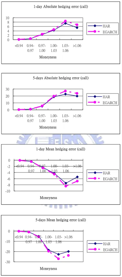
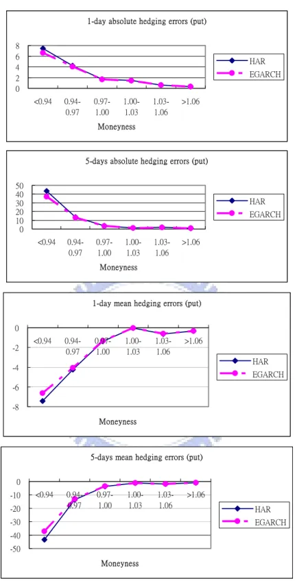
This study exhibits the empirical investigation of option hedging performance in the period from Apr. 2, 2007 to June 29, 2007 (totally 63 trading days). Table 6.1 and 6.2 report the out-of-sample hedging performance for call and put options, respectively. The results are also plotted in Figures 6.1 and 6.2 in terms of hedging horizon and different criteria of evaluation hedging performance of different moneyness categories. Firstly, considering hedging errors in call options, both in one-day hedging and five-days hedging, the HAR-RV model performs better than the EGARCH model for all evaluating criteria.

Secondly, in the case of put options, contrasts to the case of call options, our numerical reports exhibit the entirely different results. The HAR-RV model underperforms the EGARCH model for all evaluating criteria and different hedging horizon. However, in Figure 6.2, it is easy to discover that the difference of hedging errors between the HAR-RV model and the EGARCH model is close to zero, except for ITM put options. In sum, although the EAGRCH model performs better than HAR-RV model in put options, it does not show significant superior in hedging performance.

7. Conclusion

This thesis uses S&P500 index options data to investigate the empirical pricing and hedging performance of the HAR-RV option pricing model relative to the EGARCH option pricing model. Our results show that the HAR-RV model outperforms the EGARCH model in terms of one-day and five-days SPX call option pricing performance for all moneyness, except for OTM call options. When considering put options, the HAR-RV model exhibits smaller pricing errors for all moneyness categories in terms of the three evaluating criteria. Comparing one-day performance with five-day pricing performance, both in call and put options, it can obviously find that five-days pricing errors are bigger than one-day, consistent with the intuition that using more previous data to forecast pricing will exhibit bigger pricing bias.

Furthermore, in hedging performance, this study shows that the HAR-RV option pricing model performs better than the EGARCH option pricing model only in the case of call options for all moneyness, while worse for put options. Although the EAGRCH option pricing model performs better than the HAR-RV model in put options, it is easy to discover that the difference of hedging errors between the HAR-RV model and the EGARCH model is close to zero, except for ITM put options.

Form the above results, it implies that the HAR-RV option pricing model is superior both for call and put options in one-day and five-days pricing performance and in call option hedging performance. The EGARCH option pricing model does not show significant superiority in hedging performance for put options.

Various issues could be examined by future studies. Since this study ignores the effects of the transaction cost, the dividend, and the borrowing-lending cost, in the future, it can add these factors for the improvement of evaluating pricing and hedging performance. Additionally, in financial markets, American options are heavily traded contracts, further researches can extend to evaluate American options pricing and hedging performance by applying the HAR-RV volatility model.

Reference

Andersen, T.G., T. Bollerslev, F. X. Diebold, and P. Labys (2001). The distribution of realized exchange rate volatility. Journal of the American Statistical Association, 96, 42-55.

Andersen, T.G., T. Bollerslev, F. X. Diebold, and P. Labys (2003). Modeling and forecasting realized volatility. Econometrica, 71, 579-625.

Andersen, T. G., T. Bollerslev, and F. X. Diebold (2005). Parametric and non-parametric volatility measurement. In Handbook of Financial Econometrics (L.P Hansen and Y. A AÏt-Sahalia, eds.). Elsevier Science, New York, forthcoming.

Andersen, T. G., T. Bollerslev, and F. X. Diebold (2007). Roughing it up: Including jump components in the measurement, modeling and forecasting of return volatility. The Review of Economics and Statistics, 89(4): 701–720.

Bakshi, G., C. Cao, , and Z. Chen (1997). Empirical performance of alternative option pricing models. Journal of Finance, 52, 2003-2049.

Barnodorff-Nielsen, O.E. and N. Shephard (2004a). Power and bipower variation with stochastic volatility and jumps. Journal of Financial Econometrics, 2, 1-37.

Barnodorff-Nielsen, O.E. and N. Shephard (2004b). How accurate is the asymptotic approximation to the distribution of realized volatility. In Identification and Inference for Econometric Models. A Festschrift in Honour of T.J. Rothenberg (D. Andrews, J. Powell, P.A. Ruud, and J. Stock, eds.). Cambridge, UK: Cambridge University Press.

Barnodorff-Nielsen, O.E., S. E. Graversen, and N. Shephard (2004). Power variation and stochastic volatility: A review and some new results. Journal of Applied Probability, 41A, 133-143. Black, F. and M. Scholes (1973). The pricing of options and corporate liabilities. Journal of Political

Economy, 637-653.

Bollerslev, T. (1986). Generalized autoregressive conditional heteroskedasticity. Journal of Econometrics, 31, 307-327.

Bollerslev, T. and H. O. Mikkelsen. (1999). Long-term equity anticipation securities and stock market volatility dynamics. Journal of Econometics, 92, 75-99.

Corsi, F. (2003). A simple long memory model of realized volatility. Manuscript, University of Southern Switzerland.

Dumas, B., J. Fleming, and R. Whaley (1998). Implied volatility functions: Empirical tests. Journal of Finance, 53, 2059-2106.

Engle, R. and V. Ng (1993). Measuring and testing the impact of news on volatility. Journal of Finance, 48, 1749-1778.

Haynes H., M. Yung, and H. Zhang (2003). An empirical investigation of the GARCH option pricing model: Hedging performance. The Journal of Futures Markets, 23, 1191-1207. Heston, S. and S. Nandi (2000). A closed-form GARCH option valuation model. Review of

Financial Studies, 13, 585-625.

Heston, S. L. (1993). A closed solution for options with stochastic volatility, with application to bond and currency options. Review of Financial Studies, 327-343.

Hull, J. and A. White (1987). The pricing of options on assets with stochastic volatilities. Journal of Finance, 42, 281-300.

Müller, U. A., M. M. Dacorogna, R. D. Davé, R. B. Olsen, O. V. Puctet, and J. von Weizsäcker (1997). Volatilities of different time resolutions - analyzing the dynamics of market components. Journal of EmpiricalFinance, 4, 213-239.

Nelson, D. (1991). Conditional heteroskedasticity in asset returns: A New approach. Econometrica, 59, 347-370.

Table 2.1

Summary Statistics of SPX in Call Options

Moneyness Full sample <0.94 0.94－0.97 0.97－1.00 1.00-1.03 1.03－1.06 >1.06

Average bid-offer option price 39.53 1.41 3.91 17.62 40.11 74.57 198.45

Minimum option price 0.40 0.40 0.40 1.23 17.00 51.80 91.50

Maximum option price 909.20 9.40 25.40 52.10 71.50 112.40 909.20

Total number of observations 2913 180 787 893 547 212 294

Note. This table summarizes the SPX call option data for the period from Apr. 2, 2007 to June 29, 2007. Moneyness is defined as S K , where S is the index level andK is the strike price.

Table 2.2

Summary Statistics of SPX in Put Options

Moneyness Full sample <0.94 0.94－0.97 0.97－1.00 1.00-1.03 1.03－1.06 >1.06

Average bid-offer option price 14.19 162.32 63.17 31.38 16.04 8.09 2.96

Minimum option price 0.40 92.10 44.70 13.30 4.40 1.85 0.40

Maximum option price 263.30 263.30 91.50 59.20 43.50 24.95 19.75

Total number of observations 4098 40 129 627 804 689 1809

Note. This table summarizes the SPX put option data for the period from Apr. 2, 2007 to June 29, 2007. Moneyness is defined asS K, where S is the index level andK is the strike price.

Table 4.1

Summary Statistic of the Parameter Estimators of the EGARCH(1,1) Option Pricing Model

Parameter Mean Standard Deviation min max

ω _{-0.1497 0.0090 -0.1719 -0.1357}

ϕ _{0.9885 0.0007 0.9865 0.9896}

θ _{-0.0859 0.0013 -0.0894 -0.0832}

γ _{0.0469 0.0030 0.0430 0.0539}

Note. The EGARCH(1,1) model parameters are estimated from daily S&P500 index return for the period from Jan. 2, 2002 to June 29, 2007.

Table 4.2

Summary Statistic of the Parameter Estimators of the HAR-RV Option Pricing Model

Parameter Mean Standard Deviation min max

0

β 7.34E-06 7.28E-08 7.21E-06 7.60E-06

( )d β 0.1078 0.0007 0.1066 0.1092 ( )W β 0.6518 0.0009 0.6492 0.6531 ( )M β 0.1518 0.0004 0.1513 0.1535

Note. The HAR-RV model parameters are estimated from daily S&P500 index return for the period from Jan. 2, 2002 to June 29, 2007.

Table 5.1

One-day Out-of-sample Valuation Error of the HAR-RV and EGARCH model for Call Options

MBIAS ($) MAE ($) RMAE (%)

Moneyness HAR EGARCH HAR EGARCH HAR EGARCH

All Mean 1.2183 -6.6982 2.341 6.7065 0.5251 0.432 Stdev 2.6455 5.7242 1.7325 5.7144 0.9155 0.29 <0.94 Mean 2.1044 -1.3544 2.2114 1.3544 2.0548 0.9544 Stdev 1.6035 1.3777 1.4517 1.3777 1.4896 0.0459 0.94-0.97 Mean 2.7476 -2.8532 2.7885 2.8561 1.1862 0.6713 Stdev 1.9222 3.0866 1.8623 3.0839 1.0654 0.2202 0.97-1.00 Mean 1.7603 -8.0779 2.5215 8.0804 0.214 0.4223 Stdev 2.4863 6.2236 1.7083 6.2204 0.2213 0.1716 1.00-1.03 Mean -0.742 -10.3007 1.8722 10.3007 0.048 0.2532 Stdev 2.3505 5.3174 1.6016 5.3174 0.0399 0.0994 1.03-1.06 Mean -1.7368 -10.0362 1.9885 10.0362 0.027 0.1336 Stdev 1.9249 4.8689 1.6623 4.8689 0.0222 0.0552 >1.06 Mean 0.7135 -6.9621 1.8003 7.0292 0.0103 0.0493 Stdev 2.2099 3.9798 1.4637 3.8597 0.0086 0.0336

Note: MBIAS, MAE, and RMAE are the mean value of the valuation error in dollars, the mean absolute valuation error in dollars, and the mean value of percentage absolute error, respectively. The parameters implied by the S&P 500 index data in our sample before the being priced date are used to calculate the forecasted call option prices. The valuation error is then calculated by comparing the observed and forecasted prices. Moneyness is defined as S K, where is the S&P

500 index level and is the strike price. The HAR-RV model follows

S X ( ) ( ) _{( )} ( ) _{( )} ( ) 1 ₀ d d W M d W t d _{t t} M t

RV+ =β +β RV +β RV +β RV The EGARCH model, under risk-neutralized probability

measure Q, has the following for ln

(

S_t S_t−1

)

= −r 0.5σ_t2+σ_{t t}z* ; ln

( )

σ_t2 =ω

( )

2

(

*

)

*

ln _{t 1} z_{t 1} z_{t 1} 2

ϕ σ θ λ γ λ

Table 5.2

One-day Out-of-sample Valuation Error of the HAR-RV and EGARCH model for Put Options

MBIAS ($) MAE ($) RMAE (%)

Moneyness HAR EGARCH HAR EGARCH HAR EGARCH

All Mean -3.1351 -3.4014 3.2432 3.9542 0.5926 0.6062 Stdev 2.4449 3.8678 2.2995 3.3003 0.376 0.35 <0.94 Mean -3.0835 7.2592 3.2796 7.8156 0.0211 0.051 Stdev 2.3018 4.1135 2.0047 2.884 0.0149 0.0214 0.94-0.97 Mean -0.9555 2.9827 1.8819 4.4101 0.03 0.0703 Stdev 2.8748 3.9734 2.3696 2.2701 0.0361 0.0336 0.97-1.00 Mean -2.1006 -2.8639 2.5954 3.9577 0.0803 0.1187 Stdev 3.1105 5.0251 2.7108 4.2164 0.069 0.105 1.00-1.03 Mean -4.0164 -5.356 4.0233 5.3848 0.2755 0.3247 Stdev 2.3631 3.8934 2.3514 3.8534 0.1527 0.1582 1.03-1.06 Mean -4.7286 -5.3064 4.7286 5.3064 0.6393 0.6519 Stdev 1.836 3.0249 1.836 3.0249 0.1654 0.117 >1.06 Mean -2.6515 -2.6843 2.6515 2.6843 0.9462 0.9333 Stdev 1.8642 2.0835 1.8642 2.0835 0.0794 0.0671

Note: MBIAS, MAE, and RMAE are the mean value of the valuation error in dollars, the mean absolute valuation error in dollars, and the mean value of percentage absolute error, respectively. The parameters implied by the S&P 500 index data in our sample before the being priced date are used to calculate the forecasted put option prices. The valuation error is then calculated by comparing the observed and forecasted prices. Moneyness is defined as S K, where is the S&P

500 index level and is the strike price. The HAR-RV model follows

S X ( ) ( ) _{( )} ( ) _{( )} ( ) 1 ₀ d d W M d W t d _{t t} M t

RV+ =β +β RV +β RV +β RV The EGARCH model, under risk-neutralized probability

measure Q, has the following for ln

(

S_t S_t−1

)

= −r 0.5σ_t2+σ_{t t}z* ; ln

( )

σ_t2 =ω

( )

2

(

*

)

*

ln _{t 1} z_{t 1} z_{t 1} 2

ϕ σ θ λ γ λ

Table 5.3

Five-days Out-of-sample Valuation Error of the HAR-RV and EGARCH model for Call Options

MBIAS ($) MAE ($) RMAE (%)

Moneyness HAR EGARCH HAR EGARCH HAR EGARCH

All Mean 1.0466 -6.8791 2.3188 6.8807 0.4982 0.4439 Stdev 2.7269 5.9339 1.7757 5.9321 0.9252 0.2943 <0.94 Mean 2.0702 -1.4232 2.174 1.4232 1.9715 0.9593 Stdev 1.6905 1.4567 1.5541 1.4567 1.67 0.0432 0.94-0.97 Mean 2.5711 -2.964 2.6148 2.9659 1.0886 0.6896 Stdev 2.0394 3.1614 1.983 3.1596 1.0898 0.2127 0.97-1.00 Mean 1.54 -8.4067 2.516 8.4083 0.2074 0.4337 Stdev 2.6742 6.5829 1.7855 6.5808 0.221 0.1755 1.00-1.03 Mean -1.0039 -10.4699 2.0695 10.4699 0.0535 0.2582 Stdev 2.4468 5.4714 1.6449 5.4714 0.043 0.1023 1.03-1.06 Mean -1.7938 -10.1156 2.0456 10.1156 0.0279 0.1345 Stdev 1.8875 5.0194 1.6098 5.0194 0.022 0.0561 >1.06 Mean 0.7048 -7.2085 1.6825 7.2143 0.0096 0.0508 Stdev 2.0332 4.1893 1.3386 4.1792 0.0074 0.0353

Note: MBIAS, MAE, and RMAE are the mean value of the valuation error in dollars, the mean absolute valuation error in dollars, and the mean value of percentage absolute error, respectively. The parameters implied by the S&P 500 index data in our sample before the being priced date are used to calculate the forecasted call option prices. The valuation error is then calculated by comparing the observed and forecasted prices. Moneyness is defined as S K, where is the S&P

500 index level and is the strike price. The HAR-RV model follows

S X ( ) ( ) _{( )} ( ) _{( )} ( ) 1 ₀ d d W M d W t d _{t t} M t

RV+ =β +β RV +β RV +β RV The EGARCH model, under risk-neutralized probability

measure Q, has the following for ln

(

S_t S_t−1

)

= −r 0.5σ_t2+σ_{t t}z* ; ln

( )

σ_t2 =ω

( )

2

(

*

)

*

ln _{t 1} z_{t 1} z_{t 1} 2

ϕ σ θ λ γ λ

Table 5.4

Five-days Out-of-sample Valuation Error of the HAR-RV and EGARCH model for Put Options

MBIAS ($) MAE ($) RMAE (%)

Moneyness HAR EGARCH HAR EGARCH HAR EGARCH

All Mean -3.2914 -3.374 3.3924 3.9616 0.597 0.5992 Stdev 2.6031 4.0096 2.4699 3.4301 0.3746 0.3529 <0.94 Mean -3.2119 7.5248 3.3169 7.7094 0.0229 0.0522 Stdev 2.1032 3.2179 1.9288 2.7331 0.0158 0.0201 0.94-0.97 Mean -1.1772 2.9189 1.9551 4.4724 0.031 0.0709 Stdev 2.7517 4.17 2.2621 2.4129 0.035 0.035 0.97-1.00 Mean -2.4959 -2.8244 2.9464 4.0092 0.0892 0.1168 Stdev 3.311 5.1399 2.9167 4.279 0.0744 0.1015 1.00-1.03 Mean -4.3455 -5.3496 4.3619 5.3783 0.2915 0.3178 Stdev 2.6307 4.1553 2.6034 4.118 0.1556 0.161 1.03-1.06 Mean -4.8635 -5.2823 4.8635 5.2823 0.654 0.6455 Stdev 2.0774 3.2576 2.0774 3.2576 0.164 0.1207 >1.06 Mean -2.6773 -2.6946 2.6773 2.6946 0.9488 0.9319 Stdev 1.9442 2.1542 1.9442 2.1542 0.0781 0.0704

Note. MBIAS, MAE, and RMAE are the mean value of the valuation error in dollars, the mean absolute valuation error in dollars, and the mean value of percentage absolute error, respectively. The parameters implied by the S&P 500 index data in our sample before the being priced date are used to calculate the forecasted put option prices. The valuation error is then calculated by comparing the observed and forecasted prices. Moneyness is defined as S K, where is the S&P

500 index level and is the strike price. The HAR-RV model follows

S X ( ) ( ) _{( )} ( ) _{( )} ( ) 1 ₀ d d W M d W t d _{t t} M t

RV+ =β +β RV +β RV +β RV The EGARCH model, under risk-neutralized probability

measure Q, has the following for ln

(

S_t S_t−1

)

= −r 0.5σ_t2+σ_{t t}z* ; ln

( )

σ_t2 =ω

( )

2

(

*

)

*

ln _{t 1} z_{t 1} z_{t 1} 2

ϕ σ θ λ γ λ

TBALE 6.1

Dynamic Delta Hedging Errors for SPX Call Options

1-Day Hedging 5-Day Hedging

Moneyness HAR EGARCH HAR EGARCH

Panel A: Absolute hedging errors

all 2.5354 2.8879 6.5231 7.3214 <0.94 0.0743 0.0813 0.2748 0.2887 0.94-0.97 0.4627 0.4825 0.9666 1.0118 0.97-1.00 2.3603 2.5071 5.1477 5.6212 1.00-1.03 4.2935 4.5678 18.6331 19.7269 1.03-1.06 7.4655 8.4452 22.7341 27.0333 >1.06 5.4789 6.7991 19.8412 23.7867

Panel B: Mean hedging errors

all -2.5186 -2.8788 -6.5115 -7.3104 <0.94 -0.0515 -0.0606 -0.1916 -0.2090 0.94-0.97 -0.4472 -0.4676 -0.9647 -1.0101 0.97-1.00 -2.3541 -2.5021 -5.1477 -5.6212 1.00-1.03 -4.2935 -4.5678 -18.6331 -19.7269 1.03-1.06 -7.4655 -8.4452 -22.7341 -27.0333 >1.06 -5.4315 -6.7949 -19.8412 -23.7867

Notes. This table presents the mean value of absolute hedging error ($), the mean value of hedging error ($) of a dynamic delta hedging strategies established daily or five days for the sample period. Delta is calculated daily using parameters implied by the index data period before the date of being priced call option. Moneyness is defined as S K, where Sis the S&P 500 index level and

TBALE 6.2

Dynamic Delta Hedging Errors for SPX Put Options

1-Day Hedging 5-Day Hedging

Moneyness HAR EGARCH HAR EGARCH

Panel A: Absolute hedging errors

all 1.4344 1.3735 4.2896 3.9560 <0.94 7.4298 6.6413 43.3687 37.0871 0.94-0.97 4.2492 4.0576 13.5614 13.0808 0.97-1.00 1.6903 1.6333 3.5925 3.4118 1.00-1.03 1.4490 1.4244 1.1197 1.0955 1.03-1.06 0.6115 0.6022 1.8794 1.8272 >1.06 0.3133 0.3127 0.9276 0.9198

Panel B: Mean hedging errors

all -1.1724 -1.1155 -4.2896 -3.9560 <0.94 -7.4298 -6.6413 -43.3687 -37.0871 0.94-0.97 -4.2492 -4.0576 -13.5614 -13.0808 0.97-1.00 -1.3714 -1.3197 -3.5925 -3.4118 1.00-1.03 -0.0179 -0.0148 -1.1197 -1.0955 1.03-1.06 -0.6115 -0.6022 -1.8794 -1.8272 >1.06 -0.3133 -0.3127 -0.9276 -0.9198

Notes. This table presents the mean value of absolute hedging error ($), the mean value of hedging error ($) of a dynamic delta hedging strategies established daily or five days for the sample period. Delta is calculated daily using parameters implied by the index data period before the date of being priced put option. Moneyness is defined as S K, where is the S&P 500 index

level and

S

1-day valuation error for call option -12 -10 -8 -6 -4 -2 0 2 4 <0.94 0.94-0.97 0.97-1.00 1.00-1.03 1.03-1.06 >1.06 moneyness MBI A S HAR EGARCH

1-da y va l ua t i on e rror for c a l l opt i on

0 2 4 6 8 10 12 <0.94 0.94-0.97 0.97-1.00 1.00-1.03 1.03-1.06 >1.06 mone yne ss MA E HAR EGARCH

1-day valuation error for call option

0.00 0.50 1.00 1.50 2.00 2.50 <0.94 0.94-0.97 0.97-1.00 1.00-1.03 1.03-1.06 >1.06 moneyness RM A E _HAR EGARCH

FIGURE 5.1 One-day forecasting errors for SPX Call Options

These figures show the 1-day forecasting errors of the HAR-RV model and the EGARCH model for SPX Call Options. The parameters implied by the S&P 500 index data in our sample before the being priced date are used to calculate the forecasted prices. The valuation error is then calculated by comparing the observed and forecasted prices. Moneyness is defined as