無線感測網路中基於儲存限制模型下的金鑰分配系統

全文

(1)國立交通大學資訊科學與工程研究所碩士論文. 無線感測網路中基於儲存限制模型下的金鑰分配系統. Key Distribution for Wireless Sensor Networks in the Bounded Storage Model. 研究生：周昆逸指導教授：曾文貴. 教授. 中華民國九十六年六月.

(2) 無線感測網路中基於儲存限制模型下的金鑰分配系統. 學生：周昆逸. 指導教授：曾文貴博士. 資訊科學與工程研究所國立交通大學. 摘要這篇論文提出了在無線感測網路中，基於儲存限制模型下的金鑰分配系統。主要分為下列兩種架構：有 Base Station 跟無 Base Station。在有 Base Station 的架構中，每一個 Base Station 所覆蓋範圍內擁有多個 Sensor Node。由 Base Station 廣播一連串的隨機字串，而每個 Sensor Node 則隨機收取某幾個字元。最後再跟鄰居節點比對共有的字元，進而得到共有的金鑰。在無 Base Station 的架構中，每個 Sensor Node 產生一連串的 Pseudorandom 的字串，並且廣播給鄰居節點，而鄰居節點則隨機收取某幾個字元。最後再將所收取的字元位置回傳給原先的節點，原先的節點可以重複產生 Pseudorandom 的字串來拿取所得到的共同字元，進而得到共有的金鑰。我們的方法最特別之處在於不需預先讀取資料，較為符合 sensor network 的系統。此外，我們也透過數學及程式模擬來分析相關結果，以及討論驗證及部署的方法。跟之前的方法比較，在連結率及安全性上我們的方法有較好的結果。. 關鍵字：無線感測網路、金鑰分配、儲存限制模型. i.

(3) Key Distribution for Wireless Sensor Networks in the Bounded Storage Model. Student: Kun-Yi Chou. Advisor: Dr. Wen-Guey Tzeng. Institute of Computer Science and Engineering National Chiao Tung University. Abstract In this paper, we propose a new key distribution system for wireless sensor networks in the bounded storage model. It contains two frameworks: with base station and without base station. In “with base station,” one base station covers several sensor nodes. The base station broadcasts random bits, and then each node randomly receives some bits and stores them. Finally, each node communicates with their neighbors and finds the common bits which are stored by the node. In “without base station,” each node generates pseudorandom bits and broadcasts them. Their neighbor randomly receives some bits and stores them. Finally, each node communicates with their original neighbor, and then their original neighbor can re-generate the pseudorandom bits and find the common bits which are stored by their neighbor. The common bits are the shared key. In our scheme, nodes don’t preload secrets, and it is easy to fit the sensor networks. Moreover, we analysis and simulate this scheme, and discuss the authentication and deployment. In the connectivity and security, the result of our scheme is better than preceding scheme.. Keywords: sensor networks, key distribution, Bounded Storage Model (BSM) ii.

(4) 銘謝在此感謝我的指導教授曾文貴教授，在我碩士班兩年的學習過程中，不只讓我在學業上受益良多，更在生活上以及言行上給我許多指導。此外，我要感謝口試委員，清大資工孫宏民教授、交大資工蔡錫鈞教授、中研院資科所呂及人教授，在論文上給予我許多良好的建議和指導，讓我的論文更加完善。除此之外我要感謝實驗室同學，仕烽和易儒的幫忙，實驗室學長姐，成康和孝盈的指導，以及實驗室學弟妹們在精神上的鼓勵。最後，我要感謝我的家人，不論在精神上或物質上都給予我極大的支持，讓我在無後顧之憂的情況下可以順利完成學業。在此，請以此文獻給我所有我想要感謝的人。. iii.

(5) Contents 摘要.................................................................................................................................i Abstract.........................................................................................................................ii 銘謝.............................................................................................................................. iii Contents .......................................................................................................................iv Chapter 1 Introduction................................................................................................1 Chapter 2 Related Work..............................................................................................4 Chapter 3 Background ................................................................................................8 3.1 Bounded Storage Model...................................................................................8 3.2 Birthday Paradigm ...........................................................................................9 3.3 Merkle Tree.................................................................................................... 11 3.4 Adversary Model............................................................................................13 Chapter 4 Protocol Description ................................................................................14 4.1 With Base Station...........................................................................................14 4.1.1 Broadcasting Phase .............................................................................15 4.1.2 Key Establishment Phase....................................................................16 4.2 Without Base Station......................................................................................16 4.2.1 Broadcasting Phase .............................................................................17 4.2.3 Key Establishment Phase....................................................................18 Chapter 5 Analysis .....................................................................................................19 5.1 Authentication for Pervious Works and Our Scheme ....................................19 5.2 Compare Two Models in Our Scheme ...........................................................20 5.3 Analysis for Our Scheme ...............................................................................21. iv.

(6) 5.3.1 Connectivity........................................................................................21 5.3.2 Security ...............................................................................................23 5.3.3 Overhead .............................................................................................27 5.4 Deployment for the Model with Base Station................................................29 Chapter 6 Simulation.................................................................................................31 Chapter 7 Conclusion ................................................................................................33 Bibliography ...............................................................................................................35 Appendix.....................................................................................................................38. v.

(7) Chapter 1 Introduction In the recent years, there are more applications for wireless sensor networks (WSN). And secret issues are more important in WSN. Key management is a major problem. With the limited computational capability, battery energy, and available memory of the sensor nodes, asymmetric cryptography (such as RSA and DDH) doesn’t suit for wireless sensor networks. If we use symmetric cryptography system for wireless sensor networks, we need a protocol to establish shared key between the sensor nodes and their neighbors. Maybe we can preload some data about the shared key before deploying the nodes, but every node doesn’t know its neighbors in pre-deployment time. So we must consider what data have been loaded by a node before deployment and what steps does a node execute after deployment. There are two naive solutions for key management: every node shares a master key and any pair of nodes shares a pair-wise key. In first scheme, every node loads a common key before deployment. If some nodes need secret communication, they can use the master key to encrypt the data and send them, and the node which received the encryption data can decrypt them by the same master key. But it isn’t security. If one node is compromised by the adversary, all communication of the networks will be known. In second scheme, one node shares a unique key with all other nodes. This scheme doesn’t have above problem, but each node must store v-1 (v is the number of. 1.

(8) sensor nodes) keys. If there are several thousands of nodes in the network, every node must store a large number of keys in their limited memory, but only their neighbor will communicate with them. Only a very small part of those keys which the node stored is useful. So those two schemes are impractical. Other solution for key management likes key distribution center (KDC). Example of such scheme likes SPINS [11]. This scheme contains a base station to distribute keys. Each node shares a key chain with a base station by μTESLA. If someone wants to communicate with other node, he can use the key which shared with the base station to convey the session key. This scheme is better than above schemes because the memory utility on the sensor node is low and it is very safe if the base station can’t be compromised. But the communication overhead between base station and other node is very heavy. In [10], it also has the same problem, so KDC isn’t the major solution. The major solution is random key distribution schemes. First paper was proposed by Eschenauer and Gligor [5]. And Chan et al. [1], Du et al. [3], and Liu and Ning [7] give some improvement for random key distribution. And based on random key distribution, other papers collocate with deployment knowledge to improve connectivity and security. We will give more detail in next session. On the other hand, Miller and Vaidya [8] proposes a new direction. They let the adversary listen limited information, and those information isn’t complete about shared key. Our scheme is similar this way. Also, we will give the detail about Miller’s scheme in Chapter 2. We propose a new scheme based on bounded storage model. The idea comes from Ding’s OT scheme [12]. Assume there is a large random string which anyone can’t store complete string (include the adversary). Each node doesn’t preloads secrets, 2.

(9) and they randomly select some indexes of the string and store the bit values of the indexes of the string. Then each pair of nodes only finds out the common indexes, and the values of the indexes will be the shared key. We discover that this scheme has better connectivity and security than random key distribution schemes. The construction of this paper is organized as follow. Chapter 2 gives some related works. Chapter 3 defines some background information which is relevant our scheme. Chapter 4 proposes two frameworks and protocols with the corresponding idea. Chapter 5 and Chapter 6 give the result about some analysis and simulation. Finally, Chapter 7 concludes this paper. And appendix gives the implementation for our scheme.. 3.

(10) Chapter 2 Related Work Eschenauer and Gligor [5] first propose the random key distribution. Before deployment, they construct a key pool which includes many keys, and every node randomly loads some keys and corresponding indexes in their storage. After deployment, each node discovers their neighbors, and exchanges the indexes of storing keys with them. If they find the common index, it means that they had the same key between each other. So this key is a pair-wise key. Based on Eschenauer – Gligor scheme, Chan, Perrig, and Song [1] propose a q-composite random key distribution scheme. They extend from one key to q-composite keys, and improve the network resilience against node capture. But every node preloads more keys form key pool. If there are more nodes to be captured, more keys are disclosed. Du, Deng, Han, and Varshney [3] use Blom’s key distribution scheme to implement threshold property. Blom’s key distribution is a matrix-based scheme. They use a public matrix G: (λ+1) × N and a private matrix D: (λ+1) × (λ+1), and compute the matrix A = ( D ⋅ G ) T . We can get a symmetric matrix K from G, D, and A: K = A ⋅ G = ( D ⋅ G)T ⋅ G = G T ⋅ D T ⋅ G = G T ⋅ D ⋅ G = ( A ⋅ G)T And we use K to distribute pair-wise keys. The node i only load the ith row of A and the ith column of G, and exchange the jth column of G with its neighbor node j. The node i can compute Kij from the ith row of A and the jth column of G, and the node j 4.

(11) can compute Kji from the jth row of A and the ith column of G. Because K is a symmetric matrix, the nodes i and j compute equal keys Kij and Kji. Liu and Ning [6] use the same notion to construct a polynomial-based key predistribution scheme. They create many bivariate λ-degree polynomial f such that f (i, j ) = f ( j , i ) . Each node loads a part of the functions which has computed with f (id , j ) , id is the identity of a node. If there are the same function with the node i and. its neighbor j, they can compute a pair-wise key from f (i, j ) = f ( j , i ) . In two previous schemes, when the number of compromised nodes is less than the threshold, the adversary can’t reconstruct the matrix A or the polynomial f. It means that the adversary has to compromise the number of nodes more than the threshold if he wants to get any pair-wise keys. On the other hand, other papers design special deployment knowledge to let each node and its neighbors have higher probability to get the same key before deployment. In [4], Du et al. propose deployment knowledge about the nodes that are likely to be the neighbors of a node. They divide the deployment area into several points, and the nodes in one point get keys from the points that are around them. It means that the node has higher probability to share common keys with its neighbors. By random key distribution with this deployment knowledge, connectivity and security are better than previous schemes. Liu, Ning, and Du [7] propose a group-based key distribution scheme. They put all nodes into several groups and each node shares unique key with other nodes in the same group. If the nodes are in different group, this scheme creates cross-group to connect them. The nodes in the same group are in different cross-groups and each node shares a unique key with other nodes in the same cross-group. If any two nodes 5.

(12) in the same group or cross-group want to communicate, they can directly use the shared key that already exists between them. If they are in different group and cross-group, they can find a middle node which is the same group with one node and the same cross-group with the other node. They can communicate or create common the key through the middle node. This scheme uses more communications to decrease storage and improve security. In [2], Chan and Perrig describe Peer Intermediaries for Key Establishment (PIKE), a class of key-establishment protocols that involves using one or more sensor nodes as a trusted intermediary to facilitate key establishment. Similar to group-based n × n areas (n is the number of sensor. scheme, they divide deployment area to. nodes). Each small area contains a node and every node shares a unique pair-wise key with other node in the same row or column. By geographic information, any two nodes can find the intermediary nodes easily and create session key by this node. Also, this scheme uses more communications to decrease storage and improve security. And in [8], Miller and Vaidya propose a novel scheme to distribute the pair-wise keys. They leverage channel diversity for sending plaintext key to their neighbor. Each node broadcasts several keys through several channels. For all time of sending keys, they change the random channel for the random time period. They assume that the adversary only records one channel in the broadcasting time. By this assumption, the adversary only heard a part of the broadcasting plaintext keys. When every node wants to receive the plaintext keys, they also record the random channel for the random time period. Finally, the node and their neighbor match their receiving keys by Bloom Filters and then find the pair-wise key. Bloom Filters is a function with several hash function. The major purpose for Bloom Filters is checking the receiving 6.

(13) keys in the storing keys or not. This scheme is different from random key distribution schemes. It is similar our scheme that the adversary can’t get complete plaintext key. And for the result, connectivity and security are much better than random key distribution scheme.. 7.

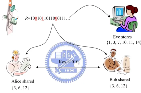
(14) Chapter 3 Background In this Chapter, we will talk about Bounded Storage Model (BSM) in Session 3.1 and Birthday Paradox for BSM in Session 3.2. In Session 3.3, we will discuss Merkle Tree to authenticate that the node isn’t a fake node. In Session 3.4, we will define adversary model.. 3.1 Bounded Storage Model In most of the public-key cryptographic systems, we assume that the adversary has limited computing power and those cryptographic systems are computational security. If a technique for unlimited computational power will be invented in the further, those cryptographic systems will be destroyed. In Bounded Storage Model, there is a station to broadcast random bits and anyone can receive all bits, include the adversary. We let two valid parties that want to establish shared key be Alice and Bob, and the adversary call Eve. Eve has unlimited power to break the cryptographic system, except for limited storage. For the broadcasting random bits R = {0,1} N , Eve can only storage αN bits with 0 < α < 1 . Alice’s and Bob’s computational ability and storage capacity are limited in polynomial time. Alice and Bob preloaded a short secret that means the indexes of the broadcast bits, and Eve doesn’t know what the secret is. When the broadcasting station begins to. 8.

(15) broadcast the random bits, Eve saves the broadcasting bits at random. Alice and Bob listen to the broadcasting bits, and they don’t need to save all of them. They just only store the bit when the index of the bit is equal to the index that they shared. We show this model in Figure3.1. Finally, Alice and Bob can get the common key from the broadcasting bits. And the probability of getting the entire common key by Eve is small. We will discuss the analysis of the probability in the later session.. R=1001011011000111…. Eve stores {1, 3, 7, 10, 11, 14}. Key is 010. Bob shared {3, 6, 12}. Alice shared {3, 6, 12} Figure 3.1: Bounded Storage Model. 3.2 Birthday Paradigm In sensor networks, we don’t know the neighbors of the node before deploying, and each node can’t preload a short secret. So we need a way of sharing common secret for a node and its neighbors. We use birthday paradigm that is used by [12] to help us to establish pair-wise keys. In our setting, we use two parties Alice and Bob, and the length of broadcasting bites is n. Each pair wants to share k bits secret, and each node must store at lost u bits 9.

(16) Lemma 1. Let Alice stores the string A, and Bob stores the string B. A and B are two independent random strings of [n] with | A |=| B |= u . Then the expected size. E[| A ∩ B |] = u 2 n .. Next, we will bound the probability of | A ∩ B | . We expect to bound it with the Chernoff-Hoeffding bounds, but it isn’t fit because the Bernoulli trials of the random bits are not independent. So we need the following version of Chernoff-Hoeffding from [14].. Lemma 2. Let Z1,…,Zu be Bernoulli trials (not necessarily independent), and let. 0 ≤ pi ≤ 1 , 1 ≤ i ≤ u . Assume that ∀i and ∀(e1 ,..., ei −1 ) ∈ {0,1}i −1 ,. Pr[ Z i = 1 | Z 1 = e1 ,..., Z i −1 = ei −1 ] ≥ pi u 2 ⎡u ⎤ Let W = ∑ pi . Then for δ < 1 , Pr ⎢∑ Z i < W ⋅ (1 − δ )⎥ < e −δ W / 2 i =1 ⎣ i=1 ⎦. (1). Corollary 1. Let A, B ⊂ [n] be two independent random subsets of [n] with. | A |=| B |= 2 kn . Then Pr[| A ∩ B |< k ] < e − k / 4 .. (2). Proof. Let u = 2 kn . Consider any fixed u-subset B ⊂ [n] , and a randomly chosen u-subset A = { A1 ,..., Au } ⊂ [n] . For i =1,…,u, let Zi be the Bernoulli trial such that Z i = 1 if and only if Ai ∈ B . Then clearly. Pr[ Z i = 1 | Z 1 = e1 ,..., Z i −1 = ei −1 ] ≥. 10. u − (i − 1) u − (i − 1) > = pi n − (i − 1) n. (3).

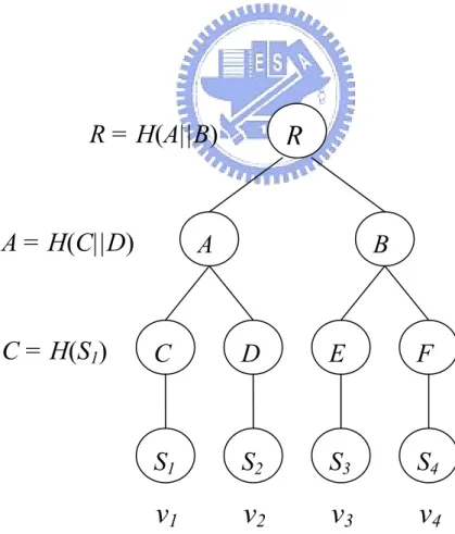
(17) u − (i − 1) 1 u 1 (1 + u ) ⋅ u u 2 W = ∑ pi > ∑ = ⋅ ∑i = ⋅ > = 2k n n i =1 n 2 2n i =1 i =1 u. u. (4). Therefore, (2) follows from (1) and (4), with δ = 1 / 2 .. Corollary 2. Let A, B ⊂ [n] be two independent random subsets of [n] with. | A |=| B |= 2 kn . Then the expected size E[| A ∩ B |] = 4k .. Proof. By lemma 1, the expected size is E[| A ∩ B |] = u 2 n , and we let u = 2 kn , then clearly E[| A ∩ B |] = (2 kn ) 2 n = 4kn / n = 4k. 3.3 Merkle Tree In our scheme, if no authentication is used, every node can sent fake date to forge the other node. So we use Merkle tree [15] to provide authentication that the neighbors of each node are not fake nodes. Assume that the number of the trusted parties is n, and we use a one-way hash function, H, to implement Merkle tree. If the party is in the trusted parties, other party can use the authenticating data of this party to authenticate him. Otherwise, other party can discovery the fake party. Each node only loads the root of the tree and log n interior nodes’ values of the tree. We will give an example in Figure 3.2. In Figure 3.2, there are four nodes: v1, v2, v3, v4, and preload secret Si. Each node generates the leaf node in Markle tree by hashing with the secret Si. For example, C = H ( S1 ) . Each interior node of the tree is generated by hashing a concatenation of. the node’s left and right children. For example, A = H (C || D ) . Repeat the steps until constructing the whole tree. 11.

(18) After constructing the whole tree, each party loads the root node and all sibling nodes of the nodes which are in the path from the user node to the root node. For example, in Figure 3.2 the path from node v1 to the root is C→A→R, and node v1 loads D and B. Then each party loads R to check the correctness. If node vi wants to authenticate its identity for its neighbors, it sends the hash value for his secret and the preloading values to the other node. In Figure 3.2, node v1 will send C and the other value D and B. The other node can compute the root from those values, and check the computing root by those data and the storing root by him being equal or not. If the result is equal, v1 is legal. Otherwise, v1 is illegal. By the Merkle Tree, every node can authenticate the other nodes.. R = H(A||B). A = H(C||D). C = H(S1). R. A. B. C. D. E. F. S1. S2. S3. S4. v1. v2. v3. v4. Figure 3.2. An example of Markle tree. 12.

(19) 3.4 Adversary Model In this session, we define adversary’s capability. Because the communication in the sensor networks is wireless, it is danger than wired networks. The adversary is easy to attack the wireless communication. We assume that the adversary has below power. He can eavesdrop to all communications and compromise any node. When he compromised one node, he could get any information about this node. And we also assume that the adversary can carry out specific active attack to the communication of the sensor networks. We define that the adversary can insert the data to forge any node. Such as pervious works, we don’t consider DoS attack. The adversary has only one restriction. His storage space has been limited. It means that he can’t store all broadcasting string into his memory. If the length of the broadcasting string is N, the adversary only has at most αN size in his storage with 0 < α < 1 . By this assumption, we can restrict the setting of the networks. For example, we limit that the adversary may not be an outside attacker with auxiliary storage. We let the adversary be an inside attacker. He can compromise the node to store the broadcasting string. And we set the size of the broadcasting string being larger than the total size of all nodes’ storage.. 13.

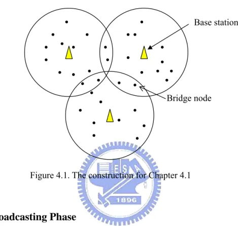
(20) Chapter 4 Protocol Description In this chapter, we talk about the protocol into two frameworks. First one includes a base station and several nodes, and the other framework includes several nodes without the base station. We describe the framework “with base station” in session 4.1 and “without base station” in session 4.2.. 4.1 With Base Station In this model, the base station has larger communication range. The nodes in this range can receive the broadcasting data from the base station. If the deployment range is larger than the base station’s communication range, we can deploy more than one base station. Each base station uses different channel to broadcast data. And there is an overlapping area between two base stations. The node in this area will be the bridge for two ranges. The bridge node can connect two different ranges with two different channels. The construction likes the Figure 4.1. We divide the scheme into two steps: Broadcasting Phase, and Key Establishment Phase. Except for the authentication data, each node doesn’t preload any secrets. After deployment, each node receives the broadcasting data from base station and stores them randomly in broadcasting phase. And then each node exchanges the authentication data and stored data in key establishment phase. By. 14.

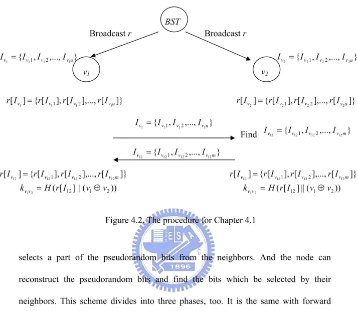
(21) those data, the node can authenticate the other nodes and establish pair-wise keys with their neighbors. In this chapter, we don’t talk about the authentication. We will give the detail in next chapter.. Base station. Bridge node. Figure 4.1. The construction for Chapter 4.1. 4.1.1 Broadcasting Phase In this phase, we deploy sensor nodes directly without preloading data. After deploying sensor nodes, we deploy base stations which have more communication range to the network. And the base station generates random bits r ∈ {0,1} and n. broadcasts them. At the same time, each node generates an index set with the size u = 2 kn . We let the index set be I v = {I v1 , I v 2 ,..., I vu } for node v. And then, when the node receives the bits, it check the indexes of all bits with the storing index set I v = {I v1 , I v 2 ,..., I vu } . If they are equal, the node stores the bits in its memory. For example, the index set I v2 = {I v2 1 , I v2 2 ,..., I v2u } was stored by the node v2. When v2 receives the broadcasting bits r, it stores the bits {r[ I v2 1 ], r[ I v2 2 ],..., r[ I v2u ]} into its storage. In next phase, we will use those bits to establish the pair-wise key. 15.

(22) 4.1.2 Key Establishment Phase In this phase, each node discovers its neighbors first. And the major steps of this phase include two steps: (1) authenticate the node’s identity (2) establish pair-wise key with their neighbors. Step 1 is based on Merkle tree. We will talk about it in next chapter. In step 2, we use the node v1 and v2 to represent the node and its neighbor. The node v1 holds the data r[ I v1 ] = {r[ I v11 ], r[ I v1 2 ],..., r[ I v1u ]} , and the node v2 holds r[ I v2 ] = {r[ I v2 1 ], r[ I v2 2 ],..., r[ I v2u ]} . We will find out the common data between r[ I v1 ] and r[ I v2 ] . First, v1 sends the index I v1 = {I v11 , I v1 2 ,..., I v1u } to v2. When v2 receives I v1 = {I v11 , I v1 2 ,..., I v1u } , it compares two index sets I v1 = {I v11 , I v1 2 ,..., I v1u } and I v2 = {I v2 1 , I v2 2 ,..., I v2u } . v2 can find the common index set I v12 = {I v12 1 , I v12 2 ,..., I v12 m } between I v1 and I v2 . Secondly, v2 sends I v12 back to v1. When v1 receives I v12 , v1 and v2 can find the same bits r[ I v12 ] = {r[ I v12 1 ], r[ I v12 2 ],..., r[ I v12 m ]} . Finally, they use hash function to compute the pair-wise key kv1v 2 = H (r[ I12 ] || (v1 ⊕ v2 )) . We show the procedure in Figure 4.2 in next page.. 4.2 Without Base Station Different from the forward model, we give a framework without base station. In this model, each node broadcasts pseudorandom bits and receives the bits from its neighbors at the same time. The steps are similar to the forward model. We use Merkle Tree to authenticate the identity, too. The different steps are in the key distribution. This model doesn’t need to find out the collision bits. It just randomly 16.

(23) BST Broadcast r. Broadcast r. I v1 = { I v11 , I v1 2 ,..., I v1u }. I v2 = { I v2 1 , I v2 2 ,..., I v2u }. v1. v2. r[ I v1 ] = {r[ I v11 ], r[ I v1 2 ],..., r[ I v1u ]}. r[ I v2 ] = {r[ I v2 1 ], r[ I v2 2 ],..., r[ I v2u ]} I v1 = { I v11 , I v1 2 ,..., I v1u }. Find. I v12 = { I v12 1 , I v12 2 ,..., I v12 m }. I v12 = { I v12 1 , I v12 2 ,..., I v12 m } r[ I v12 ] = {r[ I v12 1 ], r[ I v12 2 ],..., r[ I v12 m ]}. r[ I v12 ] = {r[ I v12 1 ], r[ I v12 2 ],..., r[ I v12 m ]}. k v1v2 = H ( r[ I12 ] || ( v1 ⊕ v 2 )). k v1v 2 = H ( r[ I12 ] || ( v1 ⊕ v2 )). Figure 4.2. The procedure for Chapter 4.1. selects a part of the pseudorandom bits from the neighbors. And the node can reconstruct the pseudorandom bits and find the bits which be selected by their neighbors. This scheme divides into three phases, too. It is the same with forward scheme: Broadcasting Phase, and Key Establishment Phase. We will give the detail in next sections.. 4.2.1 Broadcasting Phase In this phase, it is different from the Session 4.1.1. This scheme doesn’t have the base station for broadcasting. The base station broadcasting is replaced by the node broadcasting. Each node v generates pseudorandom bits rv and broadcasts them. When the. node. v2. receives. rv1. from. its. 17. neighbor v1 ,. it. stores. the. bits.

(24) rv1 [ I v2 ] = {rv1 [ I v2 1 ], rv1 [ I v2 2 ],..., rv1 [ I v2 k ]} . In this model we don’t use collision bits to find the common key, so the length of the value u is based on the security parameter of the pair-wise key, such as 32, 64, or 128 bits.. 4.2.3 Key Establishment Phase In this phase, we establish the pair-wise keys. After v2 receives rv1 , it will responds its neighbor v1 the index set I v2 = {I v2 1 , I v2 2 ,..., I v2 k } . And v1 can reconstructs. the. pseudorandom. bits. rv. and. finds. the. bits. rv1 [ I v2 ] = {rv1 [ I v2 1 ], rv1 [ I v2 2 ],..., rv1 [ I v2 k ]} . Those bits are common bits between v1 and v2 . On the other hand, v1 also stores rv2 [ I v1 ] = {rv2 [ I v11 ], rv2 [ I v1 2 ],..., rv2 [ I v1k ]} which. is broadcasted by v2 . And v2 can get the rv2 [ I v1 ] by the same way. So v1 and v2 have the common bits rv1 [ I v 2 ] and rv 2 [ I v1 ] . Finally they can compute the hashing value H ((rv1 [ I v 2 ] ⊕ rv 2 [ I v1 ]) || (v1 ⊕ v2 )) that is the pair-wise key between v1 and v2 . We have given the one way procedure in Figure 4.3.. v1. v2 I v2 = { I v2 1 , I v 2 2 ,..., I v2 k }. Generate pseudorandom rv1 , broadcast. I v2. rv1 [ I v2 ] = {rv1 [ I v2 1 ], rv1 [ I v2 2 ],..., rv1 [ I v2 k ]} = {I v2 1 , I v2 2 ,..., I v2 k }. Reconstruct pseudorandom rv1 , find rv1 [ I v 2 ] = {rv1 [ I v 2 1 ], rv1 [ I v 2 2 ],..., rv1 [ I v 2 k ]} H (( rv1 [ I v2 ] ⊕ rv2 [ I v1 ]) || (v1 ⊕ v2 )). H (( rv1 [ I v2 ] ⊕ rv2 [ I v1 ]) || (v1 ⊕ v2 )). Figure 4.3. The procedure for Chapter 4.2 18.

(25) Chapter 5 Analysis In this Chapter, we will talk about four parts: (1) analysis the authentication in pervious works and our scheme; (2) compare two models in our scheme; (3) analysis the connectivity, the security, and the overhead for our scheme; (4) discuss the deployment way for the model with base station.. 5.1 Authentication for Pervious Works and Our Scheme In key distribution schemes, the authentication is an important issue. If the scheme doesn’t include the authentication, the adversary maybe forges a legal member to break this system. We will discuss the requirement for the pervious works and our scheme. In [5], they didn’t consider the authentication for their scheme, but it is necessary. If the adversary compromised over one node, he can use the keys in those compromised nodes to forge other nodes. In [1] and [8], they have considered this problem, and they added Merkle Tree to authenticate the nodes’ identity. For our scheme, it doesn’t have any authentication in the original key distribution, and we also append Merkle Tree to authenticate the nodes’ identity. If we want to add the authentication, the node must preload some data about Merkle Tree. But in [3] and [6], the authentication has been included by their key distributions.. 19.

(26) For example in [3], the key information is contained by the row of the private matrix, and the identity of the node is related to that row. If the adversary doesn’t compromise the threshold of nodes, he can’t construct the private matrix and can’t get the identity’s row in the private matrix. If he can forge other node, he has broken the key distribution system. On the other hand, for the schemes about the deployment, the key information contains the geography in the network. If the adversary doesn’t compromise the node in that geography, he can’t get any information about that node. Such as in [2], a node has unique key for other node and communicate through the internal node. If the adversary doesn’t compromise the node in the path, he can’t get any key information about all nodes in this path. But there is a problem in Merkle Tree. If the adversary stores the authentication data for one node in previous communication, he can use those data to forge this node. So this authentication system just could be used once. Maybe we can let the node be stable. If this node is authenticated by other node, those preloaded data is unusable. And they use the agreement session key to establish an authentication system to solve this problem.. 5.2 Compare Two Models in Our Scheme We propose two models to distribute pair-wise key. Which is better? Or what environment does fit the models? We will talk about the difference in this session. The main difference is network topologic. The base station broadcasts the random bits and other node receive. The model with base station has low communication load because each node doesn’t need to broadcast bits. By this reason, 20.

(27) the power consumption for sensor nodes is lower, and the life time of the battery is much longer. But it has some secure problem. The length of the broadcasting bits is limited by bandwidth. And the bandwidth for sensor networks is small (e.g. ZigBee 250kbps). If the adversary has large storage to store all broadcasting bits, he will know all keys between each pair of all nodes. In the other model, each node broadcasts pseudorandom bits to establish the pair-wise keys. Because all nodes broadcast different pseudorandom bits, the total size of the broadcasting bits is very large. Even the adversary has enough storage to store them, and he also has a problem to listen all nodes. The adversary must deploy more nodes to listen all broadcasting bits from the legal nodes. The security in the model without base station is better than the other model. But a major problem is the life time of the battery. Broadcasting data spends high power consumption. Hence it is a trade off for the sensor network. If you want low communication load and long battery life, you can choose the model with base station. If you want more secure, you can choose the model without base station.. 5.3 Analysis for Our Scheme In this session, we will focus on the connectivity and the security. We talk about the connectivity and the security first, and then discuss the overhead in the networks.. 5.3.1 Connectivity First, we talk about the local connectivity. In the model without base station, the key is established by transmitting bits directly. It neither uses the collision nor the randomness way to get the keys. So it must establish keys after running the procedures, and the connectivity is 100%. 21.

(28) In the model with base station, the pair-wise key is established by the collision of the storing data. If we use the parameter | A |=| B |= 2 kn that are randomly chosen on [n] , we will get the result that: Pr[| A ∩ B |< k ] = e − k / 4. By this result, we can construct a system as follow: the length of the broadcasting bits is n, and n is fixed. The length of the key is k bits. And each node stores u = 2 kn bits randomly from the broadcasting bits. The size of u is depending on the length of k. Then two nodes which are neighbors check the common indexes form storing data. If the size of the collision bits is smaller than k, it mean that it is fail to establish the pair-wise key between two nodes, and this two nodes don’t connect. We consider the relation for the probability of the local connectivity and the length of the key. By the above parameters, the probability of the establishing key is 1 − e − k / 4 , and. Pr[share at least k bit]. we can get a Figure 5.1 by this formula.. (bits). k : The length of the key Figure 5.1 The probability of the connectivity 22.

(29) From the formula, we can get the result. If the length of the key is longer, the probability of establishing pair-wise keys is higher. Because n is fixed, u is depending on k. If the length of the key is longer, the size of storing string is bigger. So the probability of establishing pair-wise keys is higher when k is bigger. In Figure 5.1, we show the relation between the length of the key and the probability of establishing pair-wise keys. When k = 20, the probability of establishing the key is almost 100%. The result is much better than previous works. And from Corollary 2 in Session 3.2, the expected size of key is 4k. So the length of the pair-wise key approximates 4k. On the other hand, we often set the length of the key over 32 bits, and the probability of the local connectivity is 100%. For this result, the globe connectivity is also 100% in the range of one base station. For the total networks, if there is over one node in the overlap range of two base stations’ range, it will connect with two ranges. So the point is on the deployment of the base stations and nodes. If every overlap range has over one bridge node, the probability of the global connectivity is 100%, too. We will talk about it in Session 5.4.. 5.3.2 Security We discuss the security in this session. In previous works, the security is based on the ratio of the compromised node, because all keys are stored by all nodes. So the adversary compromises more nodes, and he will get more keys. But this discussion isn’t fit on our scheme. The security of our scheme is based on the ratio of the broadcasting bits that is stored by the adversary. We assume that the adversary can store αn bits. α is the ratio of the adversary storing the broadcasting bits, and it is a decimal between 0 and 1, and we express it by α ∈ (0,1) . n is the size of the 23.

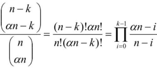
(30) broadcasting bits. The ratio that each bit is stored by the adversary is α. First, we talk about the probability Pr[get full key] that the adversary stores all bits of the key. If the key is k bits, the probability Pr[get full key] is ⎛ n−k ⎞ ⎜⎜ ⎟⎟ k −1 αn − i ⎝ αn − k ⎠ = (n − k )!αn! = ∏ n!(αn − k )! i =0 n − i ⎛n⎞ ⎜⎜ ⎟⎟ ⎝ αn ⎠. Pr[Get full key]. And we show the figure with the relation for Pr[get full key], α, and k.. k=64. k=128. k=32. α: The ratio of the adversary stored Figure 5.2 The probability getting the full key. From Figure 5.2, the probability that the adversary stores all bits of the key is very small. The adversary can’t get all bits until α > 0.8. If k is bigger, the probability is smaller. But we can’t limit the times that the adversary tests the correctness of the key. If only one bit wasn’t stored, the adversary just guessed at most two times to get 24.

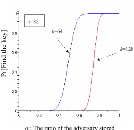
(31) the key. Hence we consider the next analysis. The adversary can compute the key if the unknown bits of the key are less than x bits. When x bits are unknown, the adversary has to test at most 2x times to compute the key. By this setting, we can get a formula that the adversary finds the key: ⎛ ⎛ k ⎞ i −1 n − αn − j k −i −1αn − j ⎞ ⎟ ∏ ⎟ n− j i =0 ⎝ ⎝ ⎠ j =0 j =0 n − j ⎠ x. ∑ ⎜⎜ ⎜⎜ i ⎟⎟∏. In this formula, we consider all case that the adversary can find the key and sum up them. The result of the formula limits the adversary’s computational power with 2x. In the Figure 5.3, we set x = 32, and the length of the key are 64 and 128bit.. Pr[Find the key]. x=32 k=64 k=128. α: The ratio of the adversary stored Figure 5.3 The probability getting the enough information for the key. When the key length is 64 bits and α is less than 0.3, the adversary can’t get any information about the key. If α is larger than 0.6, the adversary will compute all keys in this system. In 128 bits, it is more secure than 64 bits. It is perfect secret when α is 25.

(32) 0.6 and discloses all key when α is 0.82. By Session 5.3.1 and 5.3.2, the length of the key is larger, and the connectivity and security are better. By above discussion, we have ignored one fact. The expected size of collision is 4k, and we use 4k instead of k. For real model, the formula is much like: ⎛ ⎛ 4k ⎞ i −1 n − αn − j 4 k −i −1 αn − j ⎞ ⎟ ⎟⎟∏ ∏ n− j n − j ⎟⎠ i =0 ⎝ ⎝ i ⎠ j =0 j =0 x. ∑ ⎜⎜ ⎜⎜. We use this formula to update the figure as follow.. Pr[Find the key]. x=32 k=64. k=128. α: The ratio of the adversary stored Figure 5.4 The probability for the real model. Form Figure 5.4, the probability is much smaller than the probability in Figure 5.3. If less 80% bits are stored by the adversary, he can’t get any information about keys. In the model without base station, the key size is chosen by the node. Different with above discussion, we will talk about the length of the key and α. The formula is 26.

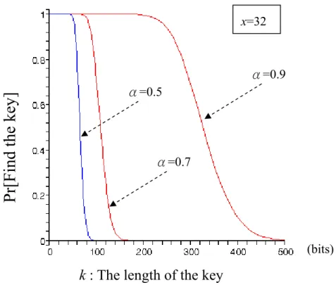
(33) the same with the above: ⎛ ⎛ k ⎞ i −1 n − αn − j k −i −1αn − j ⎞ ⎟ ∏ ⎟ n j n j − − i =0 ⎝ ⎝ ⎠ j =0 j =0 ⎠ x. ∑ ⎜⎜ ⎜⎜ i ⎟⎟∏. But we construct the different figure. We set that α is 0.5, 0.7 and 0.9, and look for the relation the length of the key:. x=32. α=0.9. Pr[Find the key]. α=0.5. α=0.7. (bits). k : The length of the key Figure 5.5 The probability for the model without base station. We can get the result from Figure 5.5. If the adversary stores 90% broadcasting bits and we want the probability 50% that the adversary can’t compute the key, we must select the length of the key with over 320 bits. We can follow our requirement to select the parameters. And we will talk about the overhead in below session.. 5.3.3 Overhead If the length of the key is large, the system is more secure. But there are some 27.

(34) problems in this setting. The length of the key is larger, and the size of storing bits is larger. By Session 3.2, we choose the storage size u = 2 kn . u concerns the length of the key and the broadcasting bits. And each node must store authentication data ( O(log v) ) from Merkle Tree. The overhead of the storage for every node is O(2 kn ) + O(log v) , and the result suites for the model with base station. In the model without base station, the storage overhead is based on the length of the key. So the overhead of the storage for every node is O(k ) + O(log v) . Next, we will discuss the communication overhead in the sensor networks. The overhead of the communication in the model with base station is n , which the length of broadcasting bits from the base station. And each node exchange the date with the indexes ( u = 2 kn ) and the authentication data ( O(log v) ). So the total communication overhand for the network is n + v(O(2 kn ) + O(log v)) , v is the number of the nodes. On the other hand, the overhead of the communication in the model without base station is the broadcasting data (n), the indexes (k), and the authentication data ( O(log v) ). So the total communication overhand for the network is v(O(n + k ) + O(log n)) . By above results, the load in model without base station is much larger than the model with base station. But maybe the size of the broadcasting bits n is different. On the computation overhead, two models are different. In the model with base station, the main load is based on finding collision. Because the index is sorted, the. ( ). load of finding collision for a node is O(u ) ≈ O n . And the computation overhead of the authentication is computing the root. It costs log v hashing. In the model without base station, the load is based on generating pseudorandom string. We assume that the computation of one bit pseudorandom generator is O(r ) , and the overhead 28.

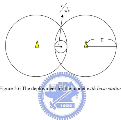
(35) for a node is O(rn ) . In the model without base station, it needs log v hashing to authenticate node’s identity, too. By above discussion, the overhead in the model with base station is smaller than the other.. 5.4 Deployment for the Model with Base Station In the model with base station, there are several base stations in the network. We call the coverage of a base station broadcasting range. The communication between different broadcasting ranges is through the node within two broadcasting ranges. In Session 4.1, we call that node bridge node. If we want that there is at least one node in the overlap of the broadcasting ranges, how do we deploy the base stations and all nodes? How many neighbors are there for a node? We will give the discussion in next paragraph. We assume the radius of a broadcast rang is r, the radius of the communication range for a node is βr, 0 < β < 1 , and there are v nodes in a broadcasting range. The area for a broadcasting range is πr 2 , and the average of the area for a node in a 2 broadcasting range is πr. v. . And we know the area of the communication range for a. node is πβ 2 r 2 . We can estimate the number of the neighbors as bellow: ⎛ 2 2 ⎞ ⎜ πβ r ⎟ − 1 = β 2v − 1 ⎜ πr 2 ⎟ v⎠ ⎝. β 2v is the number of nodes in a communication range of a node, and we subtract a node for the center of a circle. And the overlap area between two broadcasting ranges must contain at least one bridge node. It means that the overlap area is bigger than the average of the area for a node in a broadcasting range. We use the above setting. We set that the weight of the 29.

(36) overlap area is equal to the diameter of the average of the area for a node in a broadcasting range. We draw the figure in the Figure 5.6. By this setting, we can compute that the weight of the overlap area is 2r. r. v. .. v. r. Figure 5.6 The deployment for the model with base station. 30.

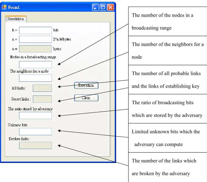
(37) Chapter 6 Simulation For our scheme, we write a program to simulate the connectivity and security. By the result of this simulation, there are some differences with the analysis in Chapter 5. We will discuss it in next paragraph. We don’t use the simulation tools for networks, such like NS2 or NCTUNS. Because we just discuss the local connectivity and security, it doesn’t need the complex program. We use C#.NET to write a simple program. We can input some parameters to set the system. Those setting include the length of the broadcasting string and the pair-wise key, the number of nodes and neighbors, the ratio of the broadcasting string which the adversary can store, and the limit for the adversary. And we can get the number of all links and connected links, the size of the storing bits for each node, and the number of the broken links. In Figure 6.1, it is the interface of the simulation program. In this simulation, the size of the broadcasting string is 2Mbytes, and we test 1~64 bits key to simulate the local connectivity. On the other hand, we test α= 0.5, α= 0.9, and x = 32 to find the probability of the security.. By this simulation, we get some results that are different with the analysis. First is about the connectivity. In Session 5.3.1, the formula is Pr[| A ∩ B |< k ] < e − k / 4 . If k is equal to 1, the probability of connectivity is e −1 / 4 . But by the result of the 31.

(38) simulation, the probability is 98%. In fact, the probability is almost 100% whatever k is. This result is better than the analysis. The connectivity isn’t an issue in our scheme. It means that the node and its neighbors will clearly establish the keys. On the other hand, the result of the security is closed to the formula ⎛ 4k ⎞ ⎟⎟(1 − α ) i α 4 k −i in Session 5.3.2. It means that our assumption is correct in i =0 ⎝ i ⎠ x. ∑ ⎜⎜. Session 5.3.2. It is much secret in real model.. The number of the nodes in a broadcasting range The number of the neighbors for a node The number of all probable links and the links of establishing key The ratio of broadcasting bits which are stored by the adversary Limited unknown bits which the adversary can compute The number of the links which are broken by the adversary. Figure 6.1 The user interface for the simulation 32.

(39) Chapter 7 Conclusion We propose a novel scheme with two models to distribute the pair-wise keys. This scheme is based on Bounded Storage Model. We assume that the adversary can’t store all broadcasting bits. By this assumption, we get the result as follow: z. If we don’t consider the authentication, each node doesn’t need preload any data.. z. The probability of the local connectivity between the node and its neighbor is almost 100%, and the globe connectivity is based on the local connectivity.. z. If the adversary can’t store all broadcasting bits, the probability that the pair-wise keys are computed by the adversary is small.. z. We give other discussions, such as authentication, deployment, simulation and difference between two models.. But there is a problem in our scheme. The rate of the data signaling in sensor networks is slow, such as ZigBee (250kbps). The length of the broadcasting bits can’t be too long. It means that the adversary can add outside storage to store all bits. Maybe we can assume that the quality of the communication isn’t good, and the adversary loses some packets when he eavesdrop the broadcasting data. We can use some equipment to interference the adversary, and let the adversary only store αn bits.. 33.

(40) We can construct a bounded storage model by using this assumption, and our protocol is useful in this model.. 34.

(41) Bibliography [1] Haowen Chan, Adrian Perrig, and Dawn Song. Random Key Predistribution Schemes for Sensor Networks. In Proceeding of the IEEE Security and Privacy Symposim 2003, May 2003. [2] Haowen Chan and Adrian Perrig, PIKE: Peer Intermediaries for Key Establishment in Sensor Networks. In Proceedings of IEEE Infocom 2005, March 2005. [3] Wenliang Du, Jing Deng, Yunghsiang S. Han, and Pramod K. Varshney. A Pair-wise Key Predistribution Scheme for Wireless Sensor Networks. In Proceedings of the 10th ACM Conference on Computer and Communication Security, page 42-51, October 2003. [4] Wenliang Du, Jing Deng, Yunghsiang S. Han, Shigang Chen, and Pramod K. Varshney, A Key Management Scheme for Wireless Sensor Networks Using Deployment Knowledge. In Proceedings of IEEE Infocom 2004, March 2004. [5] Laurent Eschenauer and Virgil D. Gligor. A Key-Management Scheme for Distributed Sensor Networks. In Proceedings of the 9th ACM Conference on Computer and Communication Security, pages 41–47, November 2002. [6] Donggang Liu and Peng Ning. Establishing Pair-wise Keys in Distributed Sensor Networks. In Proceedings of the 10th ACM Conference on Computer and. 35.

(42) Communication Security, page 52-61, October 2003. [7] Donggang Liu, Peng Ning, and Wenliang Du. Group-Based Key Pre-Distribution in Wireless Sensor Networks. In Proceedings of the 4th ACM workshop on Wireless security, page 11-20, September 2005. [8] Matthew J. Miller and Nitin H. Vaidya. Leveraging Channel Diversity for Key Establishment in Wireless Sensor Networks. In Proceedings of IEEE Infocom 2006, April 2006. [9] Ronald Watro, Derrick Kong, Sue-fen Cuti, Charles Gardiner, Charles Lynn, and Peter Kruus. TinyPK: Securing Sensor Networks with Public Key Technology. In Proceedings of 2nd ACM workshop on Security of ad hoc and sensor networks, page 59-64, October 2004. [10] Sencun Zhu, Sanjeev Setia, and Sushil Jajodia. LEAP: Efficient Security Mechanisms for Large-Scale Distributed Sensor Networks. In Proceedings of the 10th ACM Conference on Computer and Communication Security, page 62-72, October 2003. [11] Adrian Perrig, Robert Szewczyk, Victor Wen, David Culler, J. D. Tygar. SPINS: Security Protocols for Sensor Networks, In Seventh Annual International Conference on Mobile Computing and Networks, page 189-199, July 2001. [12] Yan Zong Ding. Oblivious Transfer in the Bounded Storage Model, In Proceedings of the 21st Annual International Cryptology Conference on Advances in Cryptology, page 155-170, 2002. 36.

(43) [13] U. Maurer. Conditionally-perfect secrecy and a provably-secure randomized cipher, In Journal of Cryptology, 5(1), page 53–66, 1992. [14] Y. Aumann and M. O. Rabin. Clock Construction in Fully Asynchronous Parallel Systems and PRAM Simulation, TCS, 128(1), page 3-30, 1994. [15] R. C. Merkle. A Certified Digital Signature. In Advances in Cryptology CRYPTO 1989, August 1989. [16] Farshid Delgosha and Faramarz Fekri. Threshold Key-Establishment in Distributed Sensor Networks Using a Multivariate Scheme. In Proceedings of IEEE Infocom 2006, April 2006. [17] MICAz : http://www.xbow.com/Products/productdetails.aspx?sid=164 [18] TinyOS : http://www.tinyos.net/ [19] nesC : http://nescc.sourceforge.net/. 37.

(44) Appendix For our scheme, we write a simple program on sensor networks. We use the hardware MICAz [17] to implement this system. Figure A.1 is the picture for MICAz. We give the detail specification Figure A.1 MICAz in Table A.1. MICAz. MPR2400CA. Program Flash Memory. 128k bytes. Measurement (Serial) Flash. 512k bytes. Frequency Bound. 2400 MHz to 2483.5 MHz (ISM band). Transmit data rate. 250kbps (ZigBee). Outdoor Range. 75 m to 100 m. Indoor Range. 20 m to 30 m. Battery. 2X AA batteries. User Interface. 3 LEDs (red, green, and yellow). OS. TinyOS [18]. Programming Language. nesC [19]. Table A.2 MICAz specification 38.

(45) In our program, we implement the model with base station. One base station broadcasts the data which the data structure is {index, value}, index is the order of the broadcasting bits, and value is a random bit 0 or 1. When the node receives the date from base station, it runs a probability program with the ratio u/n. It means that this program will return true with the probability u/n. When this program returns true, the node stores the data into its measurement flash, include index and value. After receiving all broadcasting bits, the node broadcasts the storing indexes to its neighbors. On the other hand, the node receives the indexes from its neighbors and compares them with the storing data. Finally, the common bits are the shared key. It is workable for our system, but the efficiency isn’t good. In the further, we will improve the data structure. Let the transmitting rate be faster, and add the utility rate of the storage.. 39.

(46)