An anisotropic spatial modeling approach for remote sensing image rectification

Remote Sensing Image Rectification

Ke-Sheng Cheng,*

,

_†

_{Hui-Chung Yeh,* and Chang-Hsuan Tsai*}

R

ectification of a remote sensing image is commonly done matically over the last decade. No remote sensing images

are free of geometric distortions and an essential

require-by applying polynomial regression models to image

coordi-nates and map coordicoordi-nates of ground control points. A ment for integrated processing of remote sensing images

and data from geographic information systems (GIS) is

major drawback of the polynomial regression model is

that it does not capture the random characteristic of ter- that they are spatially referenced. The geometric

distor-tions inherent in remote sensing images fall into two

cat-rain elevation. In fact, the distortion of a remote sensing

image is attributed to the variation of terrain elevation egories, the systematic and nonsystematic distortions.

Image rectification, a process by which the geometry of

and orbital parameters, the variations being random in

nature. A more effective approach of remote sensing im- an image area is made planimetric (Haralick, 1973;

Scho-wengerdt, 1997), must be performed prior to any

subse-age rectification is a stochastic approach that takes into

quent analyses. Many factors, such as scan skew, mirror

account the spatial variation structure of terrain

eleva-scan velocity, panoramic distortion, platform velocity,

tion. This article presents an anisotropic spatial modeling

curvature of the earth, and earth rotation, contribute to

approach of image rectification using ordinary kriging

the systematic distortions. This type of distortions can be

estimation. By considering the residuals of polynomial

rectified using data from platform ephemeris and

knowl-trend mapping as anisotropic random fields, the

pro-edge of internal sensor distortion. Nonsystematic

distor-posed approach models separately the spatial variation

tions arise from sensor system’s attitude, velocity, and

al-structures of the residuals in X and Y directions, and

em-titude, and can be corrected only through the use of

ploys the ordinary kriging method for spatial

interpola-ground control points (GCPs) (Jensen, 1986). In

particu-tion of the residual random fields. By means of a cross

lar, topographic, or relief displacement due to terrain

validation procedure, residuals of image rectification by

variation is usually the most serious of the displacement

the polynomial trend mapping, the multiquadric

interpo-types, especially in mountainous terrain (Paine, 1981).

lation function, and the ordinary kriging approaches are

There are essentially two different categories of image

compared. The ordinary kriging approach yields smallest

rectification techniques. One is the deterministic

ap-variances and root-mean-squared of mapping errors.

proach that establishes models for the nature and

magni-Elsevier Science Inc., 2000

tude of the sources of distortion and uses these models to establish correction formulae. The deterministic ap-proach relies on data of the flight parameters and the

INTRODUCTION

terrain information, and is effective when the types of Integration of remote sensing images and other geographic _{distortion are well characterized, such as that caused by} information for various applications has increased dra- _{earth rotation (Richards, 1995). The other approach of} image rectification is the statistical approach, which, by means of a GCP data set, establishes mathematical

rela-* Agricultural Engineering Department, National Taiwan

Univer-tionship between image coordinates and their

corre-sity, Taiwan, Republic of China

† Hydrotech Research Institute, National Taiwan University, Tai- sponding map coordinates using standard statistical

pro-wan, Republic of China _{cedures. These relationships can be used to correct the} Address correspondence to K.-S. Cheng, Agricultural Engineering _{image geometry irrespective of the analyst’s knowledge} Department and Hydrotech Research Inst., National Taiwan Univ.,

Tai-of the source and type Tai-of distortion (Richards, 1995).

wan, Republic of China. E-mail: [email protected]

Received 14 June 1999; revised 17 December 1999. The most widely used method in this category is the

REMOTE SENS. ENVIRON. 73:46–54 (2000)

Elsevier Science Inc., 2000 0034-4257/00/$–see front matter 655 Avenue of the Americas, New York, NY 10010 PII S0034-4257(00)00079-1

polynomial trend mapping (PTM) technique that em- polation. This study only deals with the geometric cor-ploys polynomial regression equations to relate image co- rection, and the process of pixel resampling is not part ordinates and their corresponding map coordinates. The of our investigation. We introduce the PTM and MIF order of polynomials to be used depends on the image geometric correction algorithms in this section.

sources and the terrain variation in the scene. For

air-borne images or images from areas of rugged terrain, Polynomial Trend Mapping

more severe distortions present and higher order polyno- _{Let (x, y) be the image coordinate of a pixel and (X, Y)} mials are used. In contrast, affine transformation, a first- _{be its corresponding map coordinate. Also let (Xˆ, Yˆ) be} order polynomial, may be sufficient to rectify satellite _{estimate of the map coordinate (X, Y) by a polynomial} images. An extended model of the conventional polyno- _{transformation. General form of the PTM algorithm is} mial mapping is the Hardy’s multiquadric interpolation _{given in Eqs. (1a) and (1b):}

function (MIF), which yields zero errors for coordinate

mapping at GCPs (Hardy, 1990; Star et al., 1997). The Xˆ⫽

兺

n

i⫽0

兺

i

j⫽0

aijxi⫺jyj, (1a)

MIF method employs a distance-weighting algorithm to

adjust residuals from the PTM method. _Yˆ⫽

兺

n

i⫽0

兺

i

j⫽0

bijxi⫺jyj. (1b)

Work of recent research (Malinverno, 1988; Turcotte, 1988; Chile`s, and Delfiner, 1999) has shown that terrain

Here n is the order of the polynomial model, and the variation is random in nature and can be modeled as a

ran-coefficients aij and bij are estimated by least-squares

re-dom field. Therefore, distortions raised by terrain

varia-gression analysis. The PTM is basically a statistical trend tion are randomly distributed over the spatial extent of

surface mapping model. Using a set of m GCPs, [(xk, yk);

an image. Neither the polynomial trend mapping nor the

(Xk, Yk)], k⫽1, 2, . . ., m, it finds the best-fit surface for

multiquadric interpolation function considers the spatial

the GCP data set. As was introduced earlier, low order variation structure of the terrain elevation. In this study

polynomials are used to rectify images with less geomet-we propose an alternative approach of image rectification

ric distortions, like satellite images from a flat region. by kriging. Kriging is a group of spatial interpolation

Geometric distortions like scale, translation, rotation, and methods based on the spatial correlation structure of the

skew effects can be modeled by an affine transformation random field under investigation. We adopted the

ordi-(n⫽1). Rectification of images from rugged terrain may nary kriging (OK), a linear, unbiased estimator with

min-require using higher order polynomials. However, in imum variance of estimation errors, for spatial

interpola-choosing the order of polynomials for image rectification, tion in this research.

one needs to be cautious that higher order polynomials The organization of this paper is as follows. The next

can lead to significant image distortions for regions out-section introduces the PTM and MIF algorithms of

im-side the range of the ground control points, although age rectification. The third section describes theory of the

they generally yield accurate fits in the vicinities of the ordinary kriging. The fourth section presents the algorithm

ground control points. of building a kriging model for image rectification. The fifth

section describes the method of accuracy assessment by

Multiquadric Interpolation Function

means of cross validation. An example is presented in the

sixth section to illustrate the proposed model and com- The MIF algorithm can be viewed as an extension of the pare the mapping accuracies by different approaches. PTM technique. The basic concept of this technique The final section presents some concluding remarks. is to adjust (Xˆ, Yˆ), the PTM estimate of map coordinate (X, Y), by means of a distance-weighted algorithm. The weights are determined such that the MIF mapping

er-GEOMETRIC CORRECTION ALGORITHMS

rors at ground control points are zero.

Since the statistical approach is commonly adopted for op- _{The first step of the MIF technique is to apply the} erational purpose and is independent of the platform used _{PTM model with lower degree (1 or 2) polynomials to} for data acquisition, we focus our study on modeling the _{the GCP data set, that is [Eqs. (2a) and (2b)],}

geometric distortions based on ground control point

cor-Xˆk⫽a00⫹a10xk⫹a11yk⫹a20x2k⫹a21xkyk⫹a22y2k, (2a)

respondence. Ground control points are ground features

that can be delineated on a remotely sensed image and on Yˆk⫽b00⫹b10xk⫹b11yk⫹b20x2k⫹b21xkyk⫹b22y2k. (2b)

a corresponding map. Before proceeding, readers should

Let residuals of the PTM model at ground control points, be aware that geometric correction process described in

(Xk, Yk), k⫽1, 2, . . ., m, be (dXk, dYk) [Eqs. (3a) and (3b)]:

this article is only the first phase of a complete remote

sensing georeference process. It is followed by a resampl- dXk⫽Xk⫺Xˆk, (3a)

ing process, which interpolates digital numbers of pixels of

dYk⫽Yk⫺Yˆk. (3b)

the rectified image, using techniques like nearest

m} and the following steps to establish distance-weighted _dY

0⫽

兺

m

k⫽1

f0kbk, (8b)

estimates for any non-GCP pixel (x0, y0) (Star et al., 1997).

(XˆM0, YˆM0)⫽(Xˆ0, Yˆ0)⫹(dX0, dY0). (9)

1. Calculate the distance between a non-GCP point

(x0, y0) and a GCP (xk, yk) [Eq. (4)]: _{Here, (Xˆ}

0, Yˆ0) and (XˆM0, YˆM0) are the PTM and

MIF estimates of map coordinate (X0, Y0), respec-f0k(x0, y0)⫽

√

(x0⫺xk)2⫹(y0⫺yk)2. (4)

tively. The MIF algorithm yields exact estima-2. Calculate the distance between two control points tions, that is, zero estimation errors, at ground GCP (xk, yk) and GCP (xl, yl) [Eq. (5)]: control points since Eq. (6c) has a unique

solu-tion. The residuals at (x0, y0) are determined by fkl⫽

√

(xk⫺xl)2⫹(yk⫺yl)2. (5) _{summing the distance-weighted residuals, f}

0kak

and f0kbk, k⫽1, 2, . . ., m, contributed by all

3. Model the residuals (dXk, dYk), k⫽1, 2, . . ., m, by

ground control points. the following matrix equations:

THEORY OF THE ORDINARY KRIGING

冤

dX1 dX2 ⯗ dXm

冥

⫽

冤

f11 f12 . . . f1m f21 f22 . . . f2m ⯗ ⯗ ⯗ ⯗ fm1 fm2 . . . fmm

冥

·

冤

a1 a2 ⯗ am

冥

, (6a)

The PTM is basically a traditional trend surface mapping model. It finds the best-fit surface for the GCP data set. The MIF interpolates the residuals resulted from PTM by weighting residuals contributed by each ground con-trol point. Neither method considers the spatial variation

冤

dY1 dY2 ⯗ dYm

冥

⫽

冤

f11 f12 . . . f1m f21 f22 . . . f2m ⯗ ⯗ ⯗ ⯗ fm1 fm2 . . . fmm

冥

·

冤

b1 b2 ⯗ bm

冥

, (6b)

structure of terrain elevation. The terrain variation struc-ture may be nonlinear and anisotropic. In contrast, krig-ing is a group of spatial estimation methods that take or, equivalently,

into account the spatial variation of the random field un-der investigation. In this study, we apply the most widely

D⫽

冤

D_DX

Y

冥

⫽⌿·

冤

A

B

冥

, (6c) _{used ordinary kriging to remote sensing image}

rectifica-tion and introduce briefly the theory of ordinary kriging where DX and DY represent vectors of residuals in

in this section.

X and Y directions, A and B are column vectors

Let Z(x) be a random field and z(x) be its realization of ak and bk, respectively, and ⌿ is the

inter-at a spinter-atial locinter-ation x. We wish to estiminter-ate an unknown GCP-distance matrix, that is [Eq. (6d)],

value z(x0) using observed data {z(xi), i⫽1, 2, . . ., m} and

combine them linearly with weights ki0:

⌿⫽

冤

F₀ 0_F

冥

, (6d)

z*(x0)⫽

兺

m

i⫽1

ki0z(xi). (10)

with F being the distance matrix in Eqs. (6a)

and (6b). _{Here z*(x0) represents the ordinary kriging estimate of}

4. Solve Eq. (6c) for ak and bk, k⫽1, 2, . . ., m, _{z(x0). The ordinary kriging assumes the following}

second-order stationary properties [Eqs. (11a)., (11b), and (11c)]

冤

A

B

冥

⫽⌿⫺1·

冤

DX

DY

冥

. (7) for the random field {Z(x), x苸⍀}:

E[Z(x)]⫽lZ, (11a)

The solution is unique since there are m

equa-Var[Z(x)]⫽r2

Z, (11b)

tions for m unknowns in Eqs. (6a) and (6b).

Coef-ficients ak and bk can be viewed as the residuals Cov[Z(xi),Z(xj)]⫽Cov(|xi⫺xj|), (11c)

contributed by (xk, yk) per unit length of distance

where ⍀ represents the spatial extent of the study area. from point (xk, yk). From Eq. (7), we see that ak

We require the kriging estimator to be unbiased and have and bkdepend on the geometric layout of ground

minimum variance of estimation errors, that is [Eqs. (12a) control points, which is characterized by ⌿, and _{and (12b)]}

the predetermined PTM residuals DX and DY. An

E[Z*(x0)]⫽E[Z(x0)], (12a)

implicit assumption of the MIF algorithm is that

residuals contributed by (xk, yk) are isotropic since _{minimizing Var[Z*(x0})⫺Z(x_{0)]. (12b)}

the distance matrices F and ⌿ are independent

The unbiasedness condition [Eq. (12a)] is warranted with of directions.

unit-sum weights [Eq. (13)] 5. Perform a geometric interpolation at (x0, y0) by

Eqs. (8a), (8b), and (9):

_兺

m

i⫽1 ki0⫽1. (13) dX0⫽

兺

m k⫽1 f0kak, (8a)

Table 1. Variogram Models

the two above constraints simultaneously. We achieve

this by introducing a Lagrange multiplierᐉ and minimiz- _Influence

ing Eq. (14): Model Type Formula Range Sill

Exponential c(h)⫽x[1⫺exp(⫺h/a)] 3a x

M⬅Var[z*(x0)⫺z(x0)]⫺2ᐉ

冢

兺

m

i⫽1

ki0⫺1

冣

. (14)

Spherical c(h)⫽

冦

x[3/2(h/a)⫺1/2(h/a)_x3],_, h_h⭐a_⬎a a x

By substituting

兺

m

i⫽1

ki0z(xi) for z*(x0) and differentiating M Gaussian c(h)⫽x[1⫺exp[⫺(h/a)2_]] √_{3 a x} Power c(h)⫽xha_{, a⬍2 ⫹}∞ _N/A

with respect to ki0’s and ᐉ, we obtain the ordinary

krig-ing system (Journel and Huijbregts, 1978)

兺

m

j⫽1

ki0cij⫹ᐉ⫽ci0, i⫽1, 2, . . ., m,

eters: the influence range hc, the sill c(∞), and the

nug-get C0. The influence range is the minimum distance at

兺

m

i⫽1

ki0⫽1, (15)

which two random variables Z(x) and Z(x⫹hc) become

independent. The sill is the lowest upper bound of the where cij⫽c(|xi⫺xj|) is the semivariogram, or simply the

variogram and is equal to r2

Z, the variance of Z(x). The

variogram, of the random field Z(x) and is defined in

nugget is used to model a discontinuity at the origin of Eq. (16):

the variogram. The variogram can be estimated using

ob-c(|xi⫺xj|)⫽1/2E{[Z(xi)⫺Z(xj)]2}. (16) served data {z(xi), i⫽1, 2, . . ., m}

Equation (15) can also be expressed in matrix form

cˆ(h)⫽ 1

2|N(h)|N(h)

兺

[z(x

i)⫺z(xj)]2, h⬎0 (19)

where N(h)⬅{(xi, xj): |xi⫺xj|⫽h; i,j⫽1, 2, . . ., m}. The

function cˆ(h) is often termed the experimental

vario-冤

c11 . . . c1i . . . c1m 1 ⯗ ⯗ ⯗ ⯗ ⯗ ci1 . . . cii . . . cim 1 ⯗ ⯗ ⯗ ⯗ ⯗ cm1 . . . cmi . . . cmm 1 1 . . . 1 . . . 1 0

冥

·

冤

k10 ⯗ ki0 ⯗ km0 ᐉ

冥

⫽

冤

c10 ⯗ ci0 ⯗ cm0 1

冥

. (17)

gram. Variograms are conditionally negative definite

functions (Wackernagel, 1995) and permissible models (see Table 1) or their linear combinations are often used We solve the ordinary kriging system for kriging weights to fit experimental variograms.

ki0and then substitute them into Eq. (10) to obtain zˆ(x0), In some cases the spatial variation structures or the

the kriging estimate of z(x0). The variance of the estima- variograms may vary in different directions; then the

tion error, also known as the ordinary kriging variance, random field Z(x) is said to be anisotropic. For example, is given in Eq. (18) (Journel and Huijbregts, 1978): physical or environmental parameters such as rainfall and elevation may exhibit higher degree of variation in one

r2

ok⫽E{[Z(x0)⫺Zˆ(x0)]2}

direction than in the other direction. There are two types of anisotropy, the geometric anisotropy and the zonal an-⫽ᐉ⫹

_兺

m

i⫽1

ki0ci0. (18)

isotropy. The geometric anisotropy is characterized by varying influence ranges and constant sill in different di-The variogram represents spatial variation structure of

rections. For zonal anisotropy, both the influence range the random field Z(x). Figure 1 illustrates the typical

va-and sill vary with directions. In dealing with the geomet-riogram of a random field. A vageomet-riogram has three

param-Figure 1. Typical variogram of a random field.

Figure 2. Rose diagram of an anisotropic

rically anisotropic random field, we first identify the di- transformation function. In terms of kriging, it seems in-rections of maximum and minimum spatial variation by tuitively reasonable to define a random field Z(x, y) with constructing the rose diagram, an isovariogram ellipse as (x, y) being the image coordinate and Z(x, y) the east a function of influence ranges (see Fig. 2). We then re- (or north) map coordinate, and then estimate the map scale the distance between two spatial points (x1, y1) and coordinate Z(x₀, y₀) of a non-GCP pixel at (x₀, y₀) using

(x2, y2) by using the rotation angle w and the anisotropic ground control points {(x_i, y_i), i⫽1, 2, . . ., m} and Eqs.

ratio k [Eq. (20)]: _{(10) and (17). However, since (x, y) and Z(x, y),} respec-tively, represent the image coordinate and map coordi-nate of the same pixel, the random field Z(x, y) is

non-h⫽

冪

[(x1⫺x2)cos w⫹(y1⫺y2)sin w] 2

⫹ k2_[(y

1⫺y2)cos w⫺(x1⫺x2)sin w]2 (20) stationary, and therefore violates the ordinary kriging’s

second-order stationarity assumption. This modeling ap-proach may encounter problems of fitting the experi-Then the spatial variation between any pair of (x1, y1) and

mental variograms with impermissible models, and we (x2, y2) is calculated by using the above h in the

vario-demonstrate this with an example in the Model Applica-gram model of the minimum variation axis.

tion section. In order to apply ordinary kriging to image rectification, we first model the trend present in the map-coordinate random field Z(x, y) by first-degree

poly-KRIGING APPROACH OF

nomials in Eqs. (21a) and (21b):

IMAGE RECTIFICATION

Xˆ⫽a00⫹a10x⫹a11y, (21a)

One may consider image rectification as the work of

map-ping image coordinates to map coordinates through a Yˆ⫽b00⫹b10x⫹b11y. (21b)

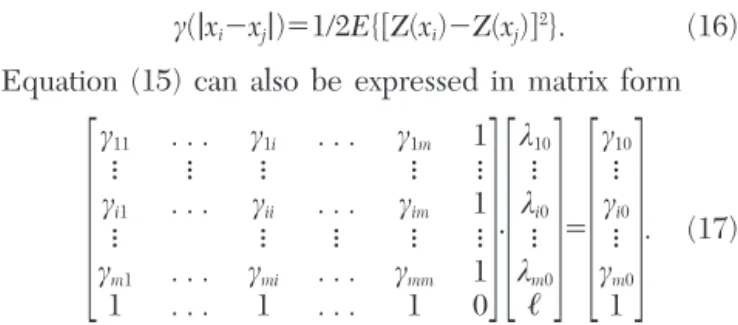
Figure 3. SPOT image of the study

We then consider the residuals dX and dY as two sepa- 3. Repeat steps 1 and 2 by returning the selected GCP and choosing another point, until all ground rate second-order stationary random fields, Z1(x, y) and

control points have been selected.

Z2(x, y), that is,

4. Calculate and compare the means and variances

Z1(x, y)⬅dX⫽X⫺Xˆ, (22a)

of (dXk, dYk), (dXMk, dYMk) and (dX*k, dY*k), k⫽1,

Z2(x, y)⬅dY⫽Y⫺Yˆ. (22b) 2, . . ., m. A better rectification model shall have

mean error close to zero and smaller variance of In the above equation, subscripts 1 and 2 correspond to

estimation errors.

X (east) and Y (north) directions, respectively. The

rea-son for using first-degree polynomials to model the trend Note that steps 1–3 of the cross validation establish of Z(x, y) is that using higher-degree polynomials in m sets of polynomial and variogram models. Based on

trend mapping may eliminate the embedding spatial vari- estimates of the cross validation procedure, we can also ation structure of the random field, and the residuals check the unbiasedness assumption of kriging [Eq. (12a)] would simply be noises. Variograms of the residual ran- and the coherence of kriging variance using Eqs. (25a) dom fields Z1(x, y) and Z2(x, y) must be estimated using and (25b):

Eq. (19) and fitted with permissible variogram models.

ME⫽1

m

兺

m

i⫽1

[z(xi)⫺z*(xi)]⬵0, (25a)

Let Z*1(x, y) and Z*2(x, y) be the ordinary kriging

esti-mates of Z1(x, y) and Z2(x, y), respectively, and they are

calculated using Eqs. (10) and (17). Finally, we calculate _MRV⫽1

m

兺

m i⫽1 [z(xi)⫺z*(xi)]2 r2 ok,i ⬵1, (25b)

the kriging estimate, (X*, Y*), of map coordinate (X, Y) using the following equations:

where r2

ok,i is the ordinary kriging variance at location xi.

X*⫽Xˆ⫹Z*1(x, y), (23a)

Y*⫽Yˆ⫹Z*2(x, y). (23b) _{Figure 4. Variogram parameter a of Z1(x, y) and Z2(x,}

y) in different directions (influence range⫽3a). The final estimation errors of the map coordinate (X, Y)

by the kriging approach are

X⫺X*⫽X⫺Xˆ⫺Z*1(x, y)⫽Z1(x, y)⫺Z*1(x, y), (24a) Y⫺Y*⫽Y⫺Yˆ⫺Z*2(x, y)⫽Z2(x, y)⫺Z*2(x, y). (24b)

Equations (24a) and (24b) indicates that the final estima-tion errors of the kriging approach (X⫺X*, Y⫺Y*) are numerically the same as the kriging errors [Z1(x, y)⫺ Z*1(x, y), Z2(x, y)⫺Z*2(x, y)].

ACCURACY ASSESSMENT

Similar to the MIF technique, the ordinary kriging is also an exact interpolator that yields zero interpolation errors at data locations. In this study we apply a cross-validation technique to verify various assumptions about the ordi-nary kriging model and the data, and also to compare the mapping accuracies of different techniques. In the cross-validation procedure one removes each sample value at a time from the observed data set, and reestimates the removed data from remaining samples using the differ-ent polynomial or variogram models. The method of cross validation for accuracy assessment works as follows:

1. From the GCP data set {(xi, yi); (Xi, Yi), i⫽1, 2,

. . ., m}, choose any one point [(xk, yk); (Xk, Yk)]

and use the remaining GCPs to estimate (Xk, Yk)

by using the PTM, MIF, and ordinary kriging techniques.

2. Calculate the estimation errors. Let (dXk, dYk),

(dXMk, dYMk), and (dX*k, dY*k) be estimation errors

of the PTM, MIF, and the kriging approaches, re-spectively.

Figure 6. Power variogram of the east map ordinate.

冤

Xˆk Yˆk

冥

⫽

冤

20.1298 ⫺2.8702 ⫺2.8702 ⫺19.6934

冥

·

冤

yxkk

冥

⫹

冤

223499.217 2699844.881

冥

. (26) We then removed the trend from Z(x, y) using Eqs. (22a) and (22b), and performed variogram analyses on residual random fields Z1(x, y) and Z2(x, y).

Variogram Modeling

Experimental directional variograms of residual random fields Z1(x, y) and Z2(x, y) were fitted with exponential

models. The principal directions of anisotropy are 0⬚– 180⬚ (E–W) and 90⬚–270⬚ (N–S) for Z1(x, y), and 30⬚–

210⬚ and 120⬚–300⬚ for Z2(x, y), as demonstrated in

Fig-Figure 5. Major and minor directional variograms of Z1(x, _{ure 4. The anisotropic ratios are 2.51 and 2.33 in the east}

y) and Z2(x, y).

and north directions, respectively. Within the study area, terrain variation is most significant in the E–W direction

MODEL APPLICATION and mild in the N–S direction, therefore, more severe

geometric distortions can be expected in the E–W direc-We apply the proposed ordinary kriging approach to a

tion. The fact that the principal directions of anisotropy test area in Northern Taiwan. The test area is 20 km by

for Z1(x, y) and Z2(x, y) are consistent with the principal

14 km in coverage, with terrain elevation ranging from

variation directions of terrain elevation demonstrates the 150 m to 1000 m above the mean sea level. A river flows

advantage of anisotropic variogram modeling. Figure 5 from east to west crossing the center of the study area.

illustrates the major and minor variograms of Z1(x, y) and

We used an unrectified SPOT satellite image (see Fig. 3)

Z2(x, y). Also, we mentioned in earlier section that

con-covering the study area to evaluate different rectification

structing variograms of the map coordinates X and Y techniques. A total of 32 ground control points were

se-without removing their trends may lead to fitting the ex-lected for model building. In the application we use the

perimental variograms with impermissible models. Fig-Universal Transverse Mercator (UTM) coordinates and

ure 6 shows the experimental variogram of the east ordi-image lines and columns for map and ordi-image

coordi-nates, respectively. nate X, along with its best-fit power model. Since the trend present in the east ordinates is not removed, the

Polynomial Trend _{best-fit power model has a degree of power exceeding}

2.0, and therefore such variogram model is not per-Using the selected GCPs, the first-degree polynomial

trend present in the study area is given in Eq. (26): missible.

Table 2. Cross Validation of Kriging Estimates

Mean Error (m) Mean of Variance Ratio

Random Field (Unbiasedness) (Variance Coherence) Anisotropic Ratio k

Z1(Easting) ⫺0.22 1.06 2.52

Table 3. Statistical Properties of Rectification Errors

Rectification Errors

PTM PTM Multiquadric

(1st Degree (2nd Degree Interpolation

Polynomials) Polynomials) Function Ordinary Kriging

Parameter dXk dYk dXk dYk dXMk dYMk dX* dY*

Mean (m) 1.37 ⫺0.28 ⫺0.18 0.15 0.22 ⫺0.75 ⫺0.22 ⫺0.15 Variance (m2_{) 7978.59 876.30 7609.78 553.95 7368.94 642.27 4803.02 581.05} RMSE (m) 87.93 29.14 85.86 23.19 84.49 24.96 68.21 23.73

65.50a _62.89a _62.30a _51.07a

Absolute Rectification Errors

PTM PTM Multiquadric

(1st Degree (2nd Degree Interpolation

Polynomials) Polynomials) Function Ordinary Kriging

Parameter |dXk| |dYk| |dXk| |dYk| |dXMk| |dYMk| |dX*| |dY*|

Mean (m) 68.26 23.09 63.69 18.57 59.56 20.62 52.57 19.00 Variance (m2_{) 3171.13 326.06 3421.97 197.98 3706.87 203.94 1950.43 208.39}

a_{Overall RMSE.}

Accuracy Assessment application. Table 3 presents the statistical properties of

rectification errors (dXk, dYk), (dXMk, dYMk), and (dX*k,

The final estimates of map coordinates for all GCPs were

dY*k) based on the cross-validation procedures outlined

calculated using the anisotropic variogram models and

in previous section. The ordinary kriging approach yields Equations (10), (17), (23a), and (23b). Table 2 presents

smaller mean, variance and root-mean-square of estima-the results of cross-validation check of kriging estimates.

tion errors than the MIF and PTM with the first-degree The unbiasedness of kriging estimates (ME⯝0) and

co-polynomials. Although PTM with the second-degree herence of kriging variance (MRV⯝1) are well satisfied,

polynomials achieves slightly smaller mean and variance indicating the anisotropic variogram models and the

as-of estimation errors in the north direction than the krig-sumption of second-order stationarity for the residual

ing approach, their differences are negligible. More im-random fields Z1(x, y) and Z2(x, y) (after variogram

re-scaling using the anisotropic ratio) are adequate for this portantly, the kriging approach achieves approximately

visit to the Mathematics Department, University of Florida,

35–40% reductions in variance of estimation errors in the

during which this study was carried out. He is also grateful to

east direction than all other models. This improvement

the Mathematics Department of University of Florida for

pro-is admirable since the terrain variation and geometric _{viding excellent research environment. We also thank the} anon-distortions are most significant in the east direction. Also, ymous reviewers for their constructive criticisms and

sugges-tions that were very helpful in revising the manuscript.

root-mean-square error (RMSE) of horizontal (east) di-rection is significantly higher than RMSE of vertical

(north) direction, indicating the rectification errors are _REFERENCES mainly contributed by errors in the east direction. The

overall RMSE of the ordinary kriging is 51.07 m, 18–22%

Chile`s, J. P., and Delfiner, P. (1999), Geostatistics—Modeling lower than RMSE of other models. Finally the kriging

Spatial Uncertainty, Wiley, New York, pp. 449–451.

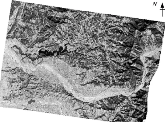
rectified image of the study area is shown in Figure 7. _{Haralick, R. M. (1973), Glossary and index to remotely sensed} image pattern recognition concepts. Pattern Recognition 5: 391–403.

CONCLUSIONS

Hardy, R. L. (1990), Theory and applications of the multiquad-ric-biharmonic method. Comput. Math. Appl. 19(8/9):163–208. In this study we compare the accuracies of image

rectifi-Jensen, J. R. (1986), Introductory Digital Image Processing—A cation by polynomial trend mapping, multiquadric

inter-Remote Sensing Perspective, Prentice-Hall, Englewood

polation function, and ordinary kriging techniques. The

Cliffs, NJ, pp. 102–105. proposed ordinary kriging approach of image rectification

Journel, A. G., and Huijbregts, C. J. (1978), Mining Geostatis-considers the mapping errors resulted from traditional

tics, Academic, London, 600 pp.

polynomial trend mapping as two stationary random _{Malinverno, A. (1988), Testing linear models of sea-floor} topog-fields. Anisotropic variogram modeling of the PTM resid- _{raphy. Pure Appl. Geophys. 131:139–156.}

uals identifies the principal variation directions and then _{Paine, D. P. (1981), Aerial Photography and Image} Interpreta-take into account the spatial variation structures of dif- tion for Resource Management, Wiley, New York, 571 pp.

Richards, J. A. (1995), Remote Sensing Digital Image Analysis, ferent directions. Results of the cross validation

demon-Springer-Verlag, Berlin, pp. 54–57. strate that ordinary kriging approach yields smaller

val-Schowengerdt, R. A. (1997), Remote Sensing—Models and Meth-ues of variance and root mean square of mapping errors

ods for Image Processing, Academic, San Diego, pp. 324–353.

than PTM and MIF techniques. This study demonstrates

Star, J. L., Estes, J. E., and McGwire, K. C. (1997), Integration the potential of applying the proposed ordinary kriging

of Geographic Information Systems and Remote Sensing,

approach to image rectification for both space-borne and _{Cambridge University Press, New York, pp. 18–25.}

airborne images. _{Turcotte, D. L. (1998), Fractals in geology and geophysics. Pure}

Appl. Geophys. 131:171–196.

Wackernagel, H. (1995), Multivariate Geostatistics,

Springer-Ver-The first author would like to thank the National Science