Large vocabulary continuous Mandarin speech recognition using finite state machine

LARGE VOCABULARY CONTINUOUS

MANDARIN SPEECH

RECOGNITION USING FINITE STATE MACHINE

Yi-Cheng Pan, Chia-Hsing Yu, and Lin-Shan Lee

Dept. of Computer Science and Information Engineering, National Taiwan

Univ., Taipei

{thomas,

davidyu, Isl)@speech.csie.ntu.edu.tw

ABSTRACT

Finite slate transducer (FST), popularly used in natural language processing (NLP) area to represent the grammar rules and the characteristics of a language, has been extensively used as the core in large vocahu-

liuy continuous speech recognition (LVCSR) in recent years. By means of FST, we can effectively compose the acoustic model, pronunciation lexicon, and lan- guage model to form a compact search space. In this paper, we present our approaches of developing

a

LVCSR decoder using FST as the core. In addition, the traditional one-pass tree-copy search algorithm is also described for comparison in terms of speed, memory requirements and achieved character accuracy.

1

INTRODUCTION

Automata theory has been developed with a long history, and relevant research is still ongoing due to its elegant frame- work and high efficiency. It has been widely used in natural language processing (NLP) area to model the grammar rules and characteristics of the language. The application of finite state automata on large vocabulary continuous speech recognition (LVCSR) was first introduced by M.Mohri[l], and a new con- cept of weighted-finite-state machine was introduced, including approaches of transforming the popularly used models such as

HMM

models and N-gram language models to finite state ma- chine[l][Z]. By means of the weighting scheme introduced, we can effectively integrate several probability likelihood functions in

a

finite state machine in a unified approach. We can then incorporate different sources of knowledge easier and reduce the complexity of the search space. Finite-state-transducer (FST) is an cxtension of finite state automata. A finite state machine can accept specific input strings (the set of strings accepted by

a

finite-state-machine is referred to as a %nguage") and a FST further has a string as output when it accepts strings. In the LVCSR system using FST as the core, we first compile three basic hiowledge sources (HMM acoustic models, pronunciation lexicon, n-gram language model) into three respective FSTs. By means of the composition algorithm, we can further integrate the three FSTs into a vast search network. A Viterhi search is then performed on this network and a best-matched path along with the recognized word sequence will be returned.

In the rest of this paper, we first review traditional one-pass tree-copy search algorithm in Section 2. We then introduce our

decoder based on FST in Section 3. The experiments and com- parison between the two different decoders in terms of speed, memory requirement and character accuracy are presented in Section 4. Finally, in Section 5 some discussions are given.

2

ONE-PASS TREE-COPY SEARCH

tree copy search algorithm.

In this section, we briefly review the traditional one-pass

In this algorithm, the search is implemented in a left-to- right, frame-synchronous fashion. We first compile a lexicon tree as shown in Fig.1, in which each arc represents a suh- syllabic HMM model and each path fmm the root to a leaf represents one or several word@) with the same pronunciation. The arcs visited by each path are the respective HMM models, of which each word is composed. in the process of searching, each active node may have several copies, where each copy represents a different language model history. The path from the root to an active node forms a partial path. If the active node is a leaf node, a new language model history is generated all the nodes having the same history are recombined and only the node with the highest score will survive while others pruned. Then from the new node having survived, we further generate a new tree copy or replace the respective existing tree root node, if the tree with specific history is already generated and the score of the new node having survived is higher than the existing one. It should be noted that we don't need to actually make several tree-copies at run-time, and the tree is just the data structure taken as a reference. In practice, only the active nodes need to be kept in the memory, where each active node represents a partial path. it should be also noted that the number of the nodes activated at each frame may increase rapidly, thus the total number of active nodes may increase exponentially. With lim- ited memory and computing power, we therefore need to further prune those active nodes with lowest scores. During pruning, we need to take the language model scores into account. At each node, there are one or several paths to go to different leaf

node(s). We pick up the leaf among them which has the highest uni-gram language model score, and this score is the look-ahead language model score for the node. Each active node is then judged by the sum of their decoding score and the look-ahead

language model score during pruning.

Fig.] An example of a tree lexicon

3

FST-BASED SEARCH ALGORITHM

3.1

FST and WFST

An FST A can be represented as a six-tuple: < Q, n, F,C,A,6

>

.

Q is the set of all states in A, while n t Q is the initial slate and F C Q is the set of all final states. is the alphabet set of input strings, while A is the alphabet set of out-

put strings. Finally,

S is the set of all possible transitions

( Q x z

+

Qx A). In speech recognition task, a weight is further attached to each transition. A weighted FST (WFST) is exactly the same

as

FST, except that

6

is now the set of all possible transitions (Qx 3 Qx Ax K ) ,where K is the set of all possi- ble weights .A transition

r

= (s[t],i[r],d[r],o[r],w[t]) can be represented by an arc from the source state

~ [ r ]

to the destination state d[t] with input label i[r] and output label o[r] and a weight w[t].ln our task,

~ [ r ]

is the log probability score.

A path in A is a sequence of consecutive transitions f l in

with d[tJ =i[r,+,],i=/, ,n-/.Transitions with an empty string E

as the input label consumes no input. A successful path

n=

f I

r,,

is the path fiom initial state i to

afinar

staie /E F. The input labels of the path

n

is the result of the concatenation of the input labels of its constituent transitions: i[ z ]=i[/,] i[t,,j,while the output labels is o[

z

]=o[t,j o[tJ

similarly. The weight associated to n i s the sum of the initial weight, the weights of its constituent transitions and the final weight of the state reached by

n.

Union operation plays an important role in the process of building the WFST for speech recognition. We can easily build small WFST pieces first, and through union operation we then bind them together to build the whole WFST.

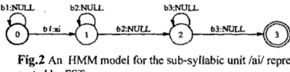
Fig2

An HMM model for the sub-syllabic unit /ail repre- sented by FST

There are three main WFST models used in the speech rec- ognition task. They are the HMM acoustic model H , the pronun- ciation lexicon model L, and the n-gram language model G. In the following sections, we will give brief descriptions about the construction of these WFST models.

3.2

HMM Acoustic Models

HMM model is widely used in speech recognition. There is a specific probability density function for each state to model the statistics of the acoustic feature vectors for that state. There are also transition probabilities between states.

Remember that the search space encoded in a WFST

is

the language accepted by the WFST, and the language is the set of all successful paths. When transforming a HMM model into a WFST, we have to shift the probability density function onto the arcs. That is, an HMM WFST is a mapping from the state prob- ability density function to the sub-syllabic acoustic model. Fig2 is a WFST to describe the subsyllable HMM model /ai/, in which there are three left-to-right HMM states. The regular ex- pression language accepted by the WFST is b,%blfb;. The out- put label "ai" can be arbitrarily attached on either arc among the

arcs

between states.

We can build a WFST for each sub-syllabic acoustic model in the same way. Then through the union operation, we can combine them together to from our HMM acoustic model H. At each final state of

H,

we additionally include an additional arc, with both input and output label E , retuming to the initial state.

Fig.3

An example partial list of the tree lexicon in FSS

3.3

Pronunciation Lexicon

The pronunciation lexicon is used to describe the pronun- ciation sequence of sub-syllabic units for each word. We can follow the same steps as we build HMM acoustic models to build a linear pronunciation lexicon. We can also further com- pile the linear lexicon into

a

tree lexicon to make it more com- pact and save the memory. Fig.3 is an example partial list of a FST for tree pronunciation lexicon.

3.4

N-gram Language Model

The most popular language model so far is the stochastic

n-gram language model. In n-gram language model, every word is assumed to be dependent only on its previous n-l words. Thus the probability of a word sequence with length N can be ap- nroximated as:

where w j is the i-rh word in the se- ability p ( ~ ,

1

d;k+l)

can be calculated from training data. However, the quantity of the corpus needed grow exponentially with the increase of n. The back-off smoothing method is usu- ally applied to compensate for the missing probability

p(w,

I

,&:+J

if the panem w;."+, does not appear in the limited training corpus, i.e., p(wj

1

IV,':;+,) = p(w,

1

w;-;+,)

,

where

2

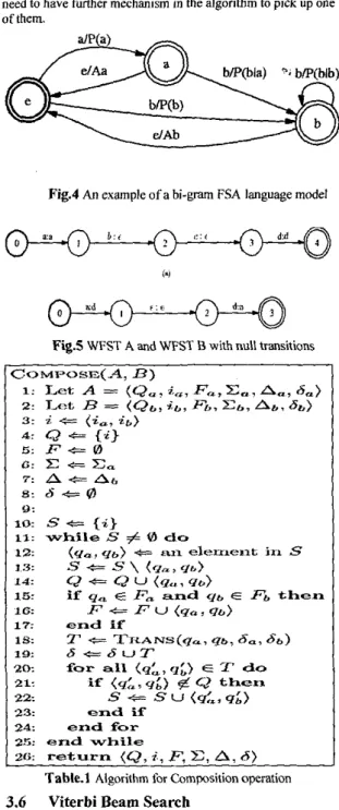
is a back-off weight (this back-off process can be repeated if 1,(:k+2 still does not appear in the corpus). In our system, n = 3, so it is a lrigram language model.

Fig.4 is a simplified WFST example with n = 2. We can note that in the WFST for the n-gram language model, every state is annotated by m words,

0

5 m S n

-

1, a s the word his- tory. Also, we use E transition to apply the back-off method mentioned above. After the introduction of E transitions, an input sequence of words might have more than one mccessful

purhs. For example, in Fig.4 if the input string is ab, then we will have two successful paths: ab, a E b, and their respective off weight. Since in the search proces$ Viterbi search is applied, we thus can further assume that the path with back-off weight should always have lower score than the one without back-off weight. Therefore, in the search process we can only get quence, w;::,, = (W,."+,,W,."+2

,...,

w # - , ), and each Prob-

,--,

",;:A,

wekhtings p(o)-p(bio),p(o).a,-p(bja), witha-ahack-

p(a)-p(bla) butneverp(a).ao

.p(bIa).

3.5

Composition Operation

Given hvo WFSTs A and B, the composition operation takes the output labels of A as the input labels of B and con- struct a new WFST C, denoted

as C =

A

0

B .

Each state of C

is composed

of

a state of A and

a

state of B, and each successful

path p of C is composed of

a

path po of A and a path pb of 9, with i[pl=i[pJ,o[pJ~i[p~,o[p~l~o[pl. and w[pl=w[pJ+ w[pJ. Table.1 is the complete composition algorithm. We need to especially note that if there are E transitions existing in both A and B, as illustrated in FigS, there will be several possible concatenation sequence ofp. and p b to form the path p of C. For example, in Fig2 if we try to go from state 4 , 1 > of C to state <3,2> of C, there are 5 different routes:

I . <

1,l

>-x 42

>-x

2,2

>+<

3,2

>

2.<

1,1>-+<

2,l

> - x

2,2

>-K

3,2

>

3.

c: 1,1

>+<

2,l >-x 3,l >-x 3,2

>

4.

<

1,l

>-K 2,2

>--1<

3,2

>

5 .

<

1,1>+<

2,1>--1< 3,2

>

6

These 5 different routes all have exactly the same score, and we need to have further mechanism in the algorithm to pick up one of them.

HMMmodelH Pronunciation

lexicon L

Fig.4

An example of a bi-gram FSA language model

# o f transitions # of states 343 589

'

349,432 287,920

Fig.5 WFST A and WFST

B with null transitions

Beamwidth(104) Real-time factor One-Pass - Tree-Copy Character Search accuracy

Tzy

S<>MPOSE<A,

B )

I: L e t A = ( Q e 3 &,

F,,

C,, A,, 6,)

2: T A : ~

R

= (Qs, it,, Fb, Et,, A,, 6s) 3: i

-+=

(ia2 ;it.) 8: F + Y ) G :

+=

E, 7: A

+=

Atz 8: d (r

8

d: Q t {i) 0 : 11: 12: 1 ~ 3 : 14: I& Io: P P U

(sa

1 40) 17: end if 1 9 6 - + = d U T 20: 21: 22. 23: end if 24: end for 25: end while as: return

(9,

i,

3;

E, A: 6)

Table.1 Algorithm for Compositionoperation

1 0

s

t {i) while

s

#

v) d o ( y a , y h ) t= all e l c r r L e l z t i n

s

c2

e=

cz

U (<i<.,

Qd

C= -9

\

( q - , qa) if qn E

Fa

and g b E 2?, then 18: 7'

+

T I C A N S ( q - , q h ,

sa,

6s) for all

<qL,q;}

E T' do if <y:z,y&)

6

Q then

s

-+=

s

U

<&*

9;)

3.6

Viterbi Beam Search

After we have composed the three WFSTs together, the HMM niodel H, the pronunciation Lexicon L and the language model G, we have

S

:=

H

o L o

G

, we can implement viterbi beam search on S. Given S = C

Q,n,

F , C ,

A,

6

>,

state q

E Q, input label 06

1

, output label X E A , respective pdf

B,

f o r o , a feature vector 0, at time I , we can compute the best score of state q at timet, S(q,r), as:

min S(q',l - I ) + B,,(o,)+w, s(q,r) = 8(<',d=(q,x,".l

where w is the transition weight from q' to 4

.

when t = 0,

10 I1 12 13 14 15 16 1.4 1.82 2.43 3.29 4.56 6.36 8.82 81.6 82.7 83.2 83.4 83.6 83.8 83.8 662 725 856 1049 1281 1558 1737 where and represent active and inactive respectively. At each timet, we call a state q with S(q,f) #

0

an ucfive state. At time 0, only the initial state is activated, and along with the tran- sition within the WFST, the number of activated states increases rapidly. With limited computing power, we can't keep all the activated states when the number of them becomes too big. We

can apply the m e beam pruning strategy as we did in the one- pass search to keep those smes with highest S(q,l) only.

FST-based search

4

EXPERIMENTS

In this section, we campare the efficiencies of tbe two de- coders, the one with one-pass tree capy search and the one with WFST, in terms of speed and memory requirements along with achieved character accuracies.

The acoustic models consist of 151 initial-final sub-syliabic units, including I12 Initials, 38 Finals, and a silence. The acous- tic features we used is 39-dimentiona1, including 13 MFCCs and delta and delta delta MFCCs. The 60K-word trigram language model is estimated on a 40M-character corpus of news from the Central News Agency at Taipei for year 1997-1999, smoothed with Good-Turing discounting by SRI Language Modeling Toolkit. The test set consists of 100 Mandain broadcast news collected from News98 Radio Station at Taipei in September 2002. The total length is 0.7 hours. The experiments are imple- mented on a computer with

AMD

Opteron 246 CPU and 8 GB RAM.

Table 2 is the number of states and arcs

of

the WFST, and Table 3 is the comparison of the running time, characYex accu- racy, and memory usage of the two search programs with differ- ent Viterhi beam widths. The comparison between them may be better examined by the two C U N e S in Fig5.and Fig.6. We can see

that at the same running time, the character accuracy of the WFST approach is always higher than the traditional one, while the growth rate of the memory usage is lower.

,,"LO, 0.74 1.04 1.45 2.03 2.74 3.69 4.80 78.0 81.3 83.1 84.2 84.8 85.2 85.3 752 779 802 824 838 850 868 factor accuracy (ME3

-

I

Tri-'an-

I

1,529,442

1

11,430,683

I

puaee model G - ~ - ~

I

H

o

L

0

G-

1

19,696,373

1

29,700,249

1

Table2 Number of states and transitions used in WFST in the experiment

Table.3 Comparison ofthe two decoders

REFERENCES

IO ’ I

---.---

[I] Mehryar Mohri, Fernando Pereira, and Michael Riley, “Weighted automata in text and speech processing,” in Extended

Finife State Models of Language: Proceedings of the ECA1’96 Workshop, Andras Komai.Ed., 1996,pp. 46-50.

121 M e b a r Mohri, “Finite-state transducers in language and

o ( -

I .

[3] Mehryar Mohri, “On some applications of finite-state su- tomata theory to natural language processing,” Journal of Na-

tional Language Engineering, vo1.2 pp. 1-20, 1996.

mg

, , , , , , ,

speech processing,” Computational Linguistics, vo1.>3,no. 2,

1

DD. - - 269-311.1997.

1-

‘PBU

-

.p-‘ [SI Mehryar Mohri, “Generic epsilon-removal and input epsi-

lon-normalization alogorithms for weighted transducers,” in

International Jounol ofFoundations ofcomuuler Science, vol.

_,--

f.,’

.

.

13, no. 1, pp. 129-143; 2002.

[6] Mehryar Mohri and Michael Riley, “A weighted pushing

algorithm for large vocabulary speech recognition,” in Proceed- ings of Eurospeech, 2001.

171 Cvril Allauzen and Mehrvar Mohri. “Generalized ootimiza-

./’

/-

?rm -

i

./”

/”

/”

[

~m

. _

.

tion algorithm for speech recognition transducers,” in Proceed-

ings ofICASSP, 2003.

am [S] Diamantina Caseiro and Isabel Tmncoso, “Using dynamic WFST composition for recognizing broadcast news,” in Pro-

r . n . 7 .

Fig.6 Comparison on memory usages between the two decoders

5

DISCUSSIONS

In this paper, we propose a miniature system to integrate different element models, H, L, G, for large vocabulary speech recognition, and we found it has comparable or better perform- ance.

M.Mohri

further proposed some methods to promote FST‘s efficiency, such as the algorithms for determination

[3],

minimization [4]. E -removal [4], and weight pushing [6]. Given

a non-deterministic WFST A, we can find an equivalent deter-

ministic WFST B aRer the determination process. A determinis- tic WFST has fewer active states than non-deterministic one. After minimization, we can further find

an

equivalent C with minimal states. These algorithms all can help us further reduce the vast search space and have the decoder find the best path in a shorter time. Since not all non-deterministic WFSTs can he determined, C.Alluzen [7] proposed an optimization algorithm

lo transfer

a

non-determinable WFST A to an equivalent B but determinable. D.Caseiro [8] also proposed a method to lower the

large number of memories required in the process of determina- tion. With these algorithms implemented, it is believed the sys- tem performances can be funher improved.