Fast Fourier Transform with Applications to Pricing Discrete European Barrier Options under Binomial and Trinomial Models

(1)

Fast Fourier Transform with Applications to

Pricing Discrete European Barrier Options

under Binomial and Trinomial Models

Hong-yiu Lin

Department of Computer Science and Information Engineering

National Taiwan University

(2)

Abstract

A derivative is a financial instrument which is constructed from other more basic underlying assets, such as bonds or stocks. With the dramatic growth of the derivatives markets, more and more derivatives have been designed and issued by financial institutions. This thesis presents a method that can be used to speed up the pricing of discrete European barrier options under binomial and trinomial tree models. Binomial tree and trinomial tree are two common and efficient models for pricing options. However, in practice, almost all barrier options are discretely monitored and the reXection principle no longer works. It seems that the only way to price discrete barrier options is to traverse the whole tree, which takes quadratic time. This thesis gives the first subquadratic-time algorithm for the problem.

(3)

List of Figures

2.1 Profit of options . . . 6

2.2 The binomial option pricing model . . . 8

3.1 A binomial tree for discrete knock-out barrier option . . . 11

3.2 The probability of a node in the binomial tree . . . 12

3.3 A binomial tree for discrete knock-out barrier option . . . 13

3.4 The basic algorithm . . . 14

4.1 The improved algorithm . . . 17

(5)

Chapter 1 Introduction

A derivative is a financial instrument which is constructed from other more basic underlying assets, such as bonds or stocks. With the dramatic growth of the derivatives markets, more and more derivatives have been designed and issued by financial institutions. Those financial innovations make the market more versatile and efficient. But on the other hand, some of those products are complicated. As a result, there are new problems with the pricing and the hedging of those derivatives.

This thesis presents a method that can be used to speed up the pricing of discrete European barrier options under binomial and trinomial tree models. Binomial tree and trinomial tree are two common and efficient models for pricing options. For barrier options, most of the pricing models assume that the underlying asset price is observed continuously.

For this type of options, the reflection principle gives a linear time solution for such case. However, in practice, almost all barrier options are discretely monitored and the reflection principle no longer works. It seems that the only way to price discrete barrier options is to traverse the whole tree, which takes quadratic time. This thesis gives the first subquadratic-time algorithm for the problem. The method relies on the discrete Fourier transform as a basic tool. Our results apply to both binomial and trinomial models.

1.1 Structures of the Thesis

This thesis is organized as follows. In Chapter 2, we give some background knowledge about financial derivatives, including the properties of derivatives, pricing models and methods. The discrete Fourier transform is also intro-duced. In Chapter 3, we describe the main question we are to solve and some basic assumptions we make for the problem. And we give a basic algorithm

(6)

which is the basis of our final improved algorithm. Chapter 4 illustrates how the improved algorithm works. Conclusion and remarks are provided in Chapter 5.

(7)

Chapter 2 Preliminaries

2.1 Option Pricing Basics

There are two basic types of options. A call option is a contract that gives its holder the right to buy the underlying asset by a expiration date for a strike price. A put option is a contract that gives its holder the right to sell the underlying asset by a expiration date for a strike price. European options can only be exercised at expiration date. In contrast, American options can be exercised any time up to the expiration date. An American option is worth as least as much as an otherwise identical European option. In most cases, it is easier to analyze European options than American options.

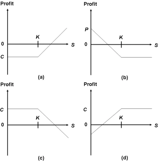
Now consider standard European options. Given the value of the under-lying asset S, the strike price K and the price of the call (put) option C (P respectively), the payoff of a long call at maturity is max(S − K, 0), and the payoff of a long put at maturity is max(K − S, 0). So the profit of a long call option at maturity is

max(S − K, 0) − C and the profit of a long put option at maturity is

max(K − S, 0) − P

Symmetrically, the profit of a short call option at maturity is min(K − S, 0) + C

and the profit of a short put option at maturity is min(S − X, 0) + P

Functions above can be expressed in Figure 2.1. Note that the calculations above ignore the time value of money.

(8)

Figure 2.1: Profit of Options. (a) A long call. (b) A long put. (c) A short call. (d) A short put.

(9)

2.2 The Black-Scholes Option Pricing Model

In 1973, Fischer Black and Myron Scholes introduced their celebrated op-tion pricing model, the Black-Scholes opop-tion pricing model. They derived a differential equation that must be satisfied by any derivative security whose underlying asset is a non-dividene-paying stock. To solve their equation, we must make the following assumptions:

1. The value of the underlying assets follows the log-normal distribution. 2. The rate of return on stock µ, the volatility of stock price σ, and the

risk-free interest rate r, are constant throughout the option’s life. 3. The short selling of securities with full use of proceeds is allowed. 4. There are no transaction costs or taxes.

5. All securities are infinitely divisible.

6. There are no dividends during the life of the option. 7. Trading is continuous.

8. There are no arbitrage opportunities.

Then Black and Scholes give the closed-form solution for European call and put options. The key formula is

∂f ∂t + rS ∂f ∂S + 1 2σ 2_S2∂2f ∂S2 − rf = 0 (2.1)

where f is the option value, S is the stock price, σ is the volatility of the stock price, and r is the continuously compounded risk-free interest rate.

The closed-form solutions for the values of European calls and puts by solving (2.1) are: C = SN (d1) − Ke−rTN (d2) P = Ke−rTN (−d 2) − SN(−d1) where d1 = ln(_KS) + (r+σ₂2)T σ√T d2 = ln(_KS) + (r−σ₂2)T σ√T = d1− σ √ T

N (x) is the probability distribution function for the standard normal distri-bution, and T is the time to maturity of the option.

(10)

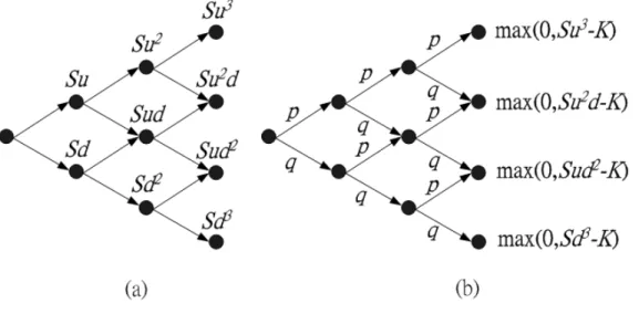
Figure 2.2: The Binomial Option Pricing Model. (a) A three-time-step binomial tree of stock prices. (b) A three-time-step binomial tree and the payoff functions at terminal nodes of a call option.

2.3 The Binomial Option Pricing Model

The binomial option pricing model is a discrete-time approximation of the continuous-time pricing model. When the current stock price is S, it can go to Su with probability q and to Sd with probability 1−q where 0 < q < 1 and ud = 1. Given S, u, d, K, ˆr and the number n of time steps to expiration, it suffices to determine the option value by backward induction. See Figure 2.2 for illustration.

2.4 Barrier Options: Continuous and Discrete

Monitoring

Barrier options are options that are activated (knocked-in) or terminated (knocked-out) when the underlying asset’s price reaches a certain price level L. For example, a knock-out call gives its holder the right to buy the underly-ing asset if the price of the underlyunderly-ing asset does not touch the barrier level L before expiration. A knock-in call is sometimes called a down-and-in option; A knock-out call is sometimes called a down-and-out option; A knock-in put is sometimes called a up-and-in option; A knock-out put is sometimes called a up-and-out option. There are also some variants of barrier options that have more than one barrier. This thesis considers single-barrier options only.

(11)

Most of the pricing models assume the underlying asset price is observed continuously. That is, at any time instant before expiration, once the price of the underlying asset touches the barrier, the knock-in or knock-out feature will take hold immediately. However, in practice, most barrier options are not continuously but discretely monitored. In other words, the underlying asset price is observed only at specified times, such as hourly, daily, or weekly. For pricing continuous barrier options under the binomial tree, there is the famous reflection principle that can be used to speed up pricing. But for the discrete case, no algorithms before this thesis have successfully lowered the complexity to subquadratic time.

2.5 Polynomial Multiplication and Discrete

Fourier Transform

One of the most frequently use algorithms in any algebraic manipulation system is multiplication. The straightforward method of multiplying two polynomials of degree n takes Θ(n2_{) time. However, better methods exist.}

Karatsuba’s method, discovered in 1962, is the first algorithm to accomplish polynomial multiplication with under O(n2_{) operations: Its time complexity}

is O(nlog₂3_).

Fact 1 Multiplication of two polynomials of degree n can be carried out in time O(nlog23).

An asymptotically better method for polynomial multiplication uses the Fast Fourier Transform (FFT). It transforms polynomials from the coefficient form to the point-value form, where multiplication can be done in O(n) time. Transforming the results back to the coefficient form then accomplishes the polynomial multiplication. The transformation takes O(n lg n) operations, thus we have the following fact.

Fact 2 Multiplication of two polynomials of degree u and v can be carried out in time O((u + v) lg(u + v)) using the FFT.

(12)

Chapter 3 Pricing European Discrete

Barrier Options with

n

Monitoring Days

3.1 Problem Statement

We consider knock-out options in this chapter. The probability distribution of terminal nodes of knock-in options can be derived from the probability distribution of knock-out options.

Under the binomial model, the stock price increases from a price S to Su with probability p and decreases to Sd with probability q = 1 − p in a time step where ud = 1. Suppose there are n monitoring days and each day is broken into m time steps. (A day is simply a fixed point in time, not necessarily a calendar day.) So there are a total of nm time steps. For simplicity, let the barrier be at L steps above the current stock price S0. That

is, the barrier price is S0uL. Assume m is even for ease of calculation. This

implies on each day, there is a node with price S0. We want to calculate the

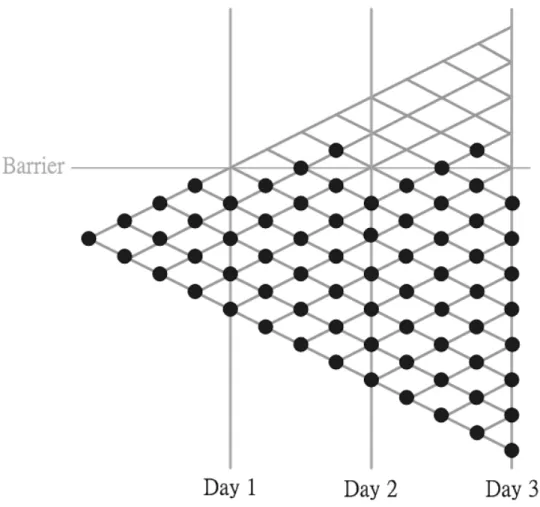
probability distribution of terminal nodes, at step nm, which is contributed by legitimate paths (i.e. those that do not touch the barrier at monitoring days). See Figure 3.1 for illustration.

Once we have the probability distribution of terminal nodes, it is easy to price European options by summing up the products of the probability and the payoff function at each terminal node and then discounting it. In general, the value of a call can be expressed as follows:

C =

PT

j=0PT,j · max(0, SujdT −j − K)

erT

(13)

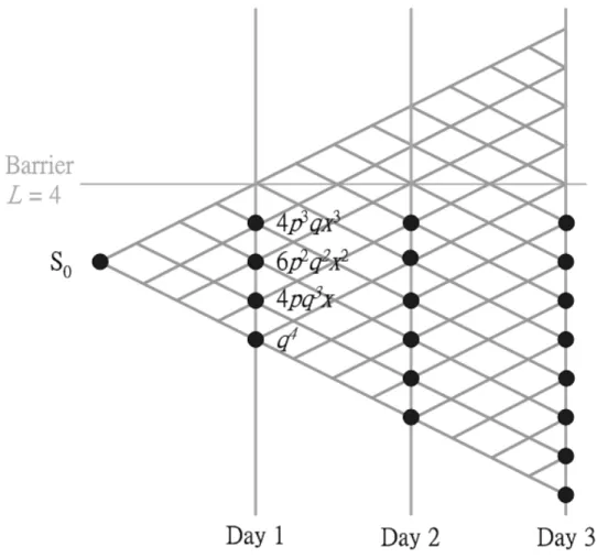
Figure 3.1: A binomial tree for discrete knock-out barrier option where n = 3 and m = 4. A filled circle means the node is legitimately reached with positive probability.

node j at time step i.

3.2 A Straightforward Solution

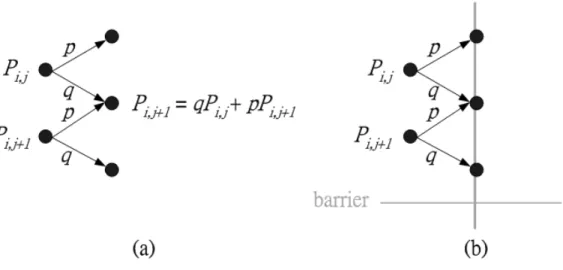
The probability of a node in the binomial tree to be reached is determined by its predecessor nodes (see Figure 3.2). A straightforward algorithm to calculate the probability distribution of terminal nodes is to calculate the probabilities of not touching the barrier of all nodes of the binomial tree step by step. Since there are O(n2_m2_{) nodes, the running time is O(n}2_m2_).

(14)

Figure 3.2: The probability of a node in the binomial tree to be legitimately reached. (a) A standard node is determined by its parents. (b) The probability of a node which touches the barrier is 0.

3.3 The Basic Algorithm

On day 1, the probability distribution (without considering the knock-out barrier) for the m + 1 nodes is

Cm_i pi_qm−i _{, for i = 0, . . . , m}

where

Cm_n = m! n!(m − n)! We can represent it as a generating function

p(x) =

m

X

i=0

Cm_i piqm−ixi

Now the price S0 is associated with the term xm/2 and the barrier L is

associated with the term xm/2+L _{since the barrier is L steps above the stock}

price S0. Because of the knock-out barrier L, anything with i ≥ m/2 + L at

a monitoring day should be set to 0. So the actual probability distribution is the truncated

(

Cm_i pi_qm−i _{for i = 0, . . . , m/2 + L − 1}

(15)

Figure 3.3: A binomial tree for discrete knock-out barrier option where n = 3 and m = 4. The probability distribution of day 1 can be seen as q1(x) = 4p3qx3 + 6p2q2x2 + 4pq3x + q4. The probability distribution of

day 2 can be obtained from q1(x)p(x).

which is represented by the generating function

q1(x) =

m/2+L−1

X

i=0

Cm_i piqm−ixi

To compute the generating function of the probability distribution of day 2, we first calculate q1(x)p(x) to obtain a polynomial of degree at most

(m/2+L)m, and for all terms that are associated with prices at or higher than barrier L (which is associated with the term xm+L), we set their coefficients to 0. See Figure 3.3.

Continue this until we reach day n. Finally, after zeroing the coefficients of xi _{with i ≥ (m/2)n + L, we obtain a generating function q}

(16)

1: Let q₀(x) := p(x) :=Pm

i=0Cmi piqm−ixi

2: _for i := 0 to n − 1 do 3: q_i+1(x) := q_i(x)p(x)

4: Set the coefficients of xj to 0 with j ≥ (m/2)(i + 1) + L 5: _{end for}

6: Output coefficients of q_n(x)

Figure 3.4: The basic algorithm.

coefficients are the probabilities we are looking for. The complete algorithm appears in Figure 3.4. In this algorithm, what we did is basically a series of n polynomial multiplications. Thus a fast polynomial multiplication method automatically results in a fast pricing algorithm.

In step 3 of Figure 3.4, the degree of p(x) is O(m) and the degree of qi(x)

is O(nm). With Fact 2 at hand, since step 3 takes time O(nm lg(nm)) and it is executed n times, the total execution time of the algorithm in

O(n · nm lg(nm)) = O(n2m lg(nm))

, whereas the running time of the straightforward algorithm is O(n2_m2_).

Lemma 1 European barrier options withn monitoring days under the bino-mial tree model can be priced in time O(n2_{m lg(nm)).}

But there is a better way. We first state a useful lemma.

Lemma 2 Multiplication of two polynomials of degree u and v where u > v can be carried out in time O(u lg v) using the FFT.

Proof: Consider the multiplication of two polynomials p(x) and q(x), where p(x) has degree u and q(x) has degree v. Since u > v, we divide

p(x) =

u

X

i=0

cixi

into u/v polynomials, p1(x), . . . , pu/v(x), where

pj(x) = jv−1

X

i=(j−1)v

cixi

for all j. Then we calculate p1(x)q(x), . . . , pu/v(x)q(x) in time

O(u

(17)

with the FFT and finally calculate p(x)q(x) = u/v X i=1 pi(x)q(x)

in time O(u). The total time complexity is therefore O(u lg v). 2

Now we use Lemma 2 to improve the running time of the algorithm in Figure 3.4. Step 3 runs in time O(nm lg m) since deg p(x) = O(m) and deg qi(x) = O(nm). The total time complexity becomes O(n2m lg m).

Lemma 3 European barrier options withn monitoring days under the bino-mial tree model can be priced in time O(n2_{m lg m).}

(18)

Chapter 4 The Improved Algorithms

4.1 The First Improvement

The basic algorithm in Figure 3.4 calculates the probabilities of the nodes day by day (see step 2 in Figure 3.4), and the loop is executed n times. We next improve the running time by making the loop execute only k times (k will be determined later) by calculating the prices every n/k days. In other words, we calculate q(i+1)n/k(x) from qin/k(x) directly. In the basic algorithm,

to calculate q(i+1)n/k(x) from qin/k(x), we must do the following:

1. Calculate qin/k(x)p(x) and chopping off terms that is higher than the

barrier to get qin/k+1(x).

2. Repeat the above procedure n/k times until q(i+1)n/k(x) is obtained.

Let qin/k(x) = inm 2k+L X j=0 cjxj

for some cj. Our new method divides qin/k(x) into two parts,

qin/k(x) = ain/k(x) + bin/k(x)

where ain/k(x) = inm 2k+L X j=(i−1)nm_2k+L cjxj and bin/k(x) = (i−1)nm_2k+L−1 X j=0 cjxj

(19)

1: Let q₀(x) := p(x) :=Pm

i=0Cmi piqm−ixi

2: Calculate [ p(x) ]n/k for later computation. 3: for i := 0 to k do

4: Divide q_in/k(x) into two parts a_in/k(x) and b_in/k(x). 5: _for j := in/k + 1 to (i + 1)n/k do

6: a_j(x) := a_j−1(x)p(x)

7: Set the coefficients of xh to 0 with h ≥ (m/2)j + L 8: _{end for}

9: b_(i+1)n/k(x) := b_in/k(x)[ p(x) ]n/k

10: q_(i+1)n/k(x) := a_(i+1)n/k(x) + b_(i+1)n/k(x) 11: _{end for}

12: Output the coefficients of q_n(x)

Figure 4.1: The improved algorithm.

As a result, the multiplication of qin/k(x) and p(x) becomes ain/k(x)p(x)+

bin/k(x)p(x). As the degree of bin/k(x) is

(i − 1)nm_2k + L − 1 and the degree of [ p(x) ]n/k _is

nm k The degree of bin/k(x)[ p(x) ]n/k is

(i − 1)nm_2k + L − 1 + nm_k = (i + 1)nm

2k + L − 1, whereas the barrier L is associated with x(i+1)nm/(2k)+L_.

Thus we can multiply [ p(x) ]n/k _{with b}

in/k(x) directly. For the ain/k(x)

part, we apply the same basic algorithm in Figure 3.4:

1. Calculate ain/k(x)p(x) and chopping off terms that are higher than

barrier to get ain/k+1(x).

2. Repeat the above procedure for n/k times until a(i+1)n/k(x)is obtained.

The improved algorithm appears in Figure 4.1.

Theorem 1 European barrier options withn monitoring days under the bi-nomial tree model can be priced in time O(mn1.5_lg(m√_n)).

(20)

Proof: Now we consider the ain/k(x) part, in step 6, deg aj−1(x) = O(nm/k)

and deg p(x) = O(m), thus its running time is O((nm/k) lg m) by Lemma 2. Since the loop of step 5 is executed n/k times, the total execution time of step 6 is O µnm k lg m · n k · k ¶ = O Ã n2 k m lg m !

For the bin/k(x) part, in step 9, deg bin/k(x) = O(nm) and deg[ p(x) ]n/k=

O(mn/k); thus its running time is O(mn lg(mn/k)) by Lemma 2. The total execution time of step 9 is

O µ mn lg µmn k ¶ · k ¶ = O µ mnk lg µmn k ¶¶

Now we set k = √n, then the execution time of the ain/k(x) part

be-comes O(mn1.5_{lg m) and the execution time of the b}

in/k(x) part becomes

O(mn1.5_lg(m√_{n)). 2}

4.2 The Final Algorithm

Observe step 5–8 of the algorithm in Figure 4.1, we use these instructions to compute a(i+1)n/k(x) from ain/k(x). The problem of computing a(i+1)n/k(x)

from ain/k(x) can be seen as a miniature of the original problem, which

computes the final probability distribution from q0(x). The method we use

in step 5–8 is exactly the basic algorithm in Figure 3.4. Now instead of using the basic algorithm, we use the improved algorithm recursively to compute a(i+1)n/k(x). We have the final algorithm in Figure 4.2.

Theorem 2 The algorithm in Figure 4.2 solves the problem of pricing Euro-pean barrier options with n monitoring days under the binomial tree model, and its running time is O(mn1+1/d_lg(mn(d−1)/d_)).

Proof: Let Fm(n, d) be the time complexity of the final algorithm with the

following arguments: FINAL ALGORITHM(q0(x), n, m, d) where deg q0(x) =

O(mn). The most exhaustive steps of the algorithm are step 7 and step 14. The running time of step 7 is

Fm(n/k, d − 1)

by definition. Thus the total time complexity of step 7 is Fm(n/k, d − 1) · k

(21)

FINAL ALGORITHM(q(x), n, m, d)

1: Let q₀(x) := q(x) 2: Let k := n1/d

3: Calculate [ p(x) ]n/k for later computation. 4: _for i := 0 to k do

5: Divide q_in/k(x) into two parts a_in/k(x) and b_in/k(x). 6: if d > 2 then

7: a_(i+1)n/k(x) :=FINAL ALGORITHM(a_in/k(x), n/k, m, d − 1)

8: _else

9: for j := in/k + 1 to (i + 1)n/k do 10: a_j(x) := a_j−1(x)p(x)

11: Set the coefficients of xh to 0 with h ≥ (m/2)j + L 12: end for

13: _{end if}

14: b_(i+1)n/k(x) := b_in/k(x)[ p(x) ]n/k

15: q_(i+1)n/k(x) := a_(i+1)n/k(x) + b_(i+1)n/k(x) 16: _{end for}

17: Output the coefficients of q_n(x)

Figure 4.2: The final algorithm. To execute the algorithm, we set q(x) = q0(x) and p(x) =Pmi=0Cmi piqm−ixi as initial arguments.

(22)

since the loop is executed k times. By Lemma 2, since deg bin/k(x) = O(mn)

and deg[ p(x) ]n/k _{= O(mn/k), the running time of step 14 is}

O(mn lg(mn/k)) . The total time complexity of step 14 is

O(mn lg(mn/k) · k)

since the loop is executed k times. We have the recursive function Fm(n, d) = Fm(n/k, d − 1)k + O(mn lg(mn/k)k) + c

for some constant c.

We use mathematical induction to complete the proof. For d = 2, the algorithm is exactly the same algorithm in Figure 4.1, and its performance is

Fm(n, 2) = O(mn1+1/2lg(mn1/2))

by Theorem 1. Now suppose for d = r, the running time of the final algorithm is

Fm(n, r) = O(mn1+1/rlg(mnr−1/r))

For d = r + 1, the total time complexity of step 7 is Fm(n/k, r) · k = O µ m³_n1/(r+1)n ´1+1/r lg(mn1−1/r_{) · (n}1/(r+1)₎¶ = O³mn1+1/(r+1)_lg(mn(r−1)/r₎´

by assumption on d = r and k = n1/(r+1)_{. For the b}

in/k(x) part, in step 14,

since deg bin/k(x) = O(mn) and deg[ p(x) ]n/k = O(mn/k) = O(mnr/(r+1)),

the total complexity of step 14 is

O³mn lg(mnr/(r+1)_{) · n}1/(r+1)´= O³mn1+1/(r+1)lg(mnr/(r+1))´ Thus the running time of the whole algorithm when d = r + 1 becomes

Fm(n, r + 1)

= Fm(n/k, r)k + mn lg(mn/k)k + c

= O³mn1+1/(r+1)_lg(mn(r−1)/r₎´_{+ O}³_mn1+1/(r+1)_lg(mnr/(r+1)₎´_{+ c}

= O³mn1+1/(r+1)_lg(mnr/(r+1)₎´

. By mathematical induction, we know that the running time of the algorithm is

O³mn1+1/dlg(mn(d−1)/d)´ for all integer d > 1. 2

(23)

Corollary 1 European barrier options with n monitoring days under the binomial tree model can be priced in time O(mn1+ǫ_lg(mn1−ǫ_{)) for all ǫ > 0.}

Proof: _{For all ǫ > 0, there exists an integer d such that 1/d ≤ ǫ. By} Theorem 2, the running time of the algorithm in Figure 4.2 is

O(mn1+1/dlg(mn(d−1)/d)) which is also in

O(mn1+ǫlg(mn1−ǫ)) 2

(24)

Chapter 5 Conclusion

In previous chapters, we consider only binomial tree models for the problem. However, in most situations, the trinomial tree pricing model has better accu-racy and faster than binomial ones. The intuition of treating the probability distribution of a time step as a generating function works well on the trino-mial model, too. Under the trinotrino-mial tree model, the current stock price can go up with probability pu, go down with probability pd and be fixed with

probability pm = 1 − pu− pd. We can change the generating function p(x) to

be

(pux2+ pmx + pd)m

and the remaining computation and analysis are the same on both models. Though Corollary 1 gives a theoretical upper bound of the problem, Im-plementation issues remain. First of all, the fast Fourier transform is hard to implement, and it requires that the degree of the polynomials be the power of 2. Since the algorithm recursively calls itself for a lot of times, the upper bound is meaningful only when n is very large, perhaps larger than practical use. However, there is an alternative, Karatsuba’s algorithm for polynomial multiplication. Since Karatsuba’s method is easier to implement, it might be a substitution in practice, but its theoretical time complexity will not be as good as the FFT method.

(25)

Bibliography

[1] Thomas H. Cormen, Charles E. Leiserson and Ronald L. Rivest Intro-duction to Algorithms. MIT Press, 1989, 776–800.

[2] Keith O. Geddes, Stephen R. Czapor and George Labahn Algorithms for Computer Algebra Kluwer Academic Publishers, 1992, 111–149. [3] John C. Hull Options, Futures and Other Derivatives. 4th ed. Englewood

Cliffs, NJ: Prentice-Hall, 1999.

[4] S. G. Kuo “On pricing of discrete barrier options.” Statistica Sinica, Vol 13 (2003), 955–964.

[5] Yuh-Daih Lyuu Funancial Engineering and Computation: Principles, Mathematics, Algorithms. Cambridge Univ. Press, 2002.

Fast Fourier Transform with Applications to Pricing Discrete European Barrier Options under Binomial and Trinomial Models