漸進式準可篩除項目集探勘之研究

國立高雄大學資訊工程學系(研究所)

碩士論文

漸進式準可篩除項目集探勘之研究

The Study of Incremental Quasi-erasable Itemset Mining

研究生：陳盧宏 撰

指導教授：洪宗貝 博士

論文審定書

致謝

兩年的研究所生活很快就過去，在這兩年研究所中，有許多艱辛的時刻，而最為艱 辛的時刻，就是本論文的完成。本論文得以完成，首先要感謝指導教授洪宗貝老師。我 感謝老師這兩年來孜孜不倦的教導，在最後論文撰寫的階段，更努力看我不完美的論文， 也給予許多鼓勵，使我同時有繼續努力的動力。另一方面，我也會繼續努力的遵循和實 踐老師所給予的教誨。因為這些教誨在未來在任何方面都可以使我有更上一層的成長。 接著，我也要感謝在我口試時，百忙之中抽空來給予我論文許多指正與建議的口試委員 們。 感謝實驗室裡許多一同認真的夥伴，平時大家一起分擔實驗室的事物，包括昆毅學 長在論文剛開始教授相關知識，還有元慶學長、世祺、冀正、仁豪和雨棠的加油鼓勵， 最後，宇喬學弟、秉洋學弟、佳哲學弟、翔維學弟等人在口試時間的付出，這些都是大 家在實驗室的共同回憶。 最後，我也要感謝自己的母親和奶奶，從小到大的扶養我，還有家裡所有的親人， 在求學階段的不斷支持我，才有現在的我，在最後的寫論文階段，也更感謝我舅舅花費 時間來看我的論文題目，幫助啟蒙我對我論文題目的不解，如果我沒有這麼多人的幫助， 不會有過去的自己，也不會有現在的自己，更不會有未來的自己。 雖然這感謝詞並非文辭並茂，但因為有這麼多人的幫助，我才有把論文繼續完成的 動力，由衷感謝一路上陪伴的人們，最後，以此論文向大家分享。

漸進式準可篩除項目集探勘之研究

指導教授：洪宗貝 博士 國立高雄大學資訊工程所 學生：陳盧宏 國立高雄大學資訊工程所 摘要 資料探勘主要是從大量資料中獲得一些有用的資訊。目前已有很多著名的資料探勘 演算法被提出，其中尤以 Apriori 演算法最常被應用，它依據項目的出現頻率來推導 出高頻項目集和關聯規則。和高頻項目集之探勘相反，可篩除項目集是用於生產規劃， 主要是要找出那些被去除也不會影響利潤的項目集。正式而言，如果一個項目集其用 於生產的利潤比例會小於或等於所給定的最高利潤比例門檻值則稱為是可以被篩除的 項目集。由於生產過程中，具不同成分(項目)的新產品可能隨時會加進來生產，若以 原來的批次探勘演算法重做處理以得到最即時的可篩除項目集將會相當耗時。在過去， 有人提出一個架構在快速更新策略的漸進式可篩除項目集探勘方法來減少維護可篩除 項目集的時間。在那方法中，假如一個項目集在原始資料庫中不是可篩除項目集，而 在新進產品中是可篩除項目集時，則必須重新掃描原始資料庫才能決定它最後是否為 可篩除項目集。因此，在本論文中，我們提出ε-準可篩除項目集的概念並且用它來增 進探勘的效能。當一個項目集的利潤比例大於最大可篩除比例門檻值 r 且小於或等於 r + ε，則被稱為 ε-準可篩除項目集。原始資料或新資料中的項目集都可被分成可篩除、 ε-準可篩除、和不可篩除三種，因此組合起來會有九種情況，而每種情況會有其所對 應的方式去處理。我們也證明了當新進資料的數量是少量時，所提的方法可以明顯減

少重掃原始資料庫的次數，最後我們也做實驗來驗證其效能。

關鍵字: 資料探勘、可篩除項目集、ε-準可篩除項目集、漸進式探勘、最大利潤比例

The Study of Incremental Quasi-erasable Itemset Mining

Advisor: Dr.Tzung-Pei Hong

Institute of Computer Science and Information Engineering National University of Kaohsiung

Student: Lu-Hung Chen

Institute of Computer Science and Information Engineering National University of Kaohsiung

ABSTRACT

Data mining gathers useful information from a big amount of data. There are some well-known mining algorithms, among which the apriori algorithm is the most commonly used. It derives frequent itemsets and association rules according to the occurring frequencies of items. Contrary to frequent-itemset mining, erasable-itemset mining used in production planning identifies itemsets (or components) that, if removed, would not affect profits. Formally, an itemset is erasable if its gain ratio is equal to or smaller than a given maximum gain-ratio threshold r. Since new products with different components may be added, the original batch algorithm will waste time in gathering up-to-date erasable itemsets. In the past, an incremental erasable-itemset mining algorithm based on the fastupdate (FUP) strategy was proposed to reduce maintenance time. In that approach, if an itemset is non-erasable in an original database but erasable in a new product, re-scanning is needed to determine whether it is finally erasable. In this thesis, we propose the concept of the ε-quasi-erasable itemsets and use it to improve mining performance. We define an itemset as ε-quasi-erasable if its gain ratio is larger than the maximum erasable ratio threshold r, but is less than or equal to r + ε. The itemsets in both the original database and the new product can then be divided into erasable, ε-quasi-erasable, and non-erasable. Thus, there are nine combinations that are then

processed in their own ways. We also prove the proposed approach can significantly reduce the rescanning number if the number of new products is small. Experiments are finally made to verify performance.

Keywords: data mining, erasable itemset, ε-quasi-erasable itemset, incremental mining, maximum gain-ratio threshold.

Content

論文審定書... i 致謝………... ii 摘要………... iii ABSTRACT ... v Content………,vii List of Figures ... i List of Tables ... xi Chapter 1 Introduction ... 1

1.1 Background and Motivation ... 1

1.2 Thesis Organization... 2

Chapter 2 Review and Related Work ... 4

2.1 Erasable Itemsets Mining ... 4

2.2 Pre-Large Itemset Mining ... 5

2.3 Survey of Erasable Itemset Mining Algorithm ... 6

Chapter 3 The Incremental Algorithm for Mining ε-quasi-Erasable Itemsets ... 7

3.1 Main idea ... 7

3.2 The Notation ... 10

3.3 The Proposed Incremental ε-quasi-erasable Itemset Mining Algorithm ... 12

3.4 An Example ... 17

Chapter 4 Experiments and Analysis ... 24

4.2 Experimental Results... 25 Chapter 5 Conclusion and Future Work ... 39 References ………40

List of Figures

Figure 3.1: The concept of ε-quasi-erasable-itemsets ... ..8 Figure 4.1: The way to generating a product base ... 25 Figure 4.2: The execution time of the three algorithms for N = 1000 ... 26 Figure 4.3:The numbers of erasable and ε-quasi-erasable itemsets obtained by the

proposed algorithm for N= 1000 ... 27 Figure 4.4: The execution time of the three algorithms for N = 5000 ... 28 Figure 4.5:The numbers of erasable and ε-quasi-erasable itemsets obtained by the

proposed algorithm for N = 5000 ... 29 Figure 4.6: The execution time of the first inserting run for different N values ... 29 Figure 4.7: The number of itemsets of inserting different number of products in the first

inserting run ... 30 Figure 4.8: The number of erasable itemsets of the proposed algorithm with different r

and ε = 0.05 ... 31 Figure 4.9: The execution time of the proposed algorithm with different thresholds and ε

= 0.05 ... 31 Figure 4.10:The number of ε-quasi-erasable itemsets of the proposed algorithm with

different ε and r = 0.5.. ... 32 Figure 4.11: The execution time of the proposed algorithm with different ε and r = 0.5 ... …33 Figure 4.12: The execution time of different number of itemsets with ε = 0.05 and r = 0.5 ... 33

Figure 4.13: The execution time of different number of original products with no rescanning original products in first inserting run ... 34 Figure 4.14: The execution time of different number of original products with no rescanning original products in first inserting run ... 34

List of Tables

Table 2.1: A Simple Example of a Product Dataset ... 3

Table 2.2: The history of existing algorithms for mining erasable itemsets ... 6

Table 3.1: Nine cases arising from adding new products to existing products... 8

Table 3.2: The erasable itemsets found from Table 2.1 ... 18

Table 3.3: Two newly inserted products in the example ... 18

Table.3.4: The 0.05-quasi-erasable itemsets found from Table 2.1 ... 18

Table 3.5: The gain values of the four 1-itemsets in new products ... 19

Table 3.6: The gain values of the erasable 2-itemsets in CN2 ... 21

Table 3.7: The gain values of the ε-quasi-erasable 2-itemsets in EN2 ... 22

Table 3.8: The final updated erasable itemsets ... 23

Table 3.9: The final updated ε-quasi-erasable itemsets ... 23

Chapter 1

Introduction

1.1 Background and Motivation

Mining useful information from big data has become very important to many applications recently. In 2009, Deng et al. defined the problem of erasable-itemset (EI) mining [7], which was an adaptation of the apriori algorithm [2]. Different from the apriori algorithm [2], the EI mining algorithm [7] is used for finding itemsets (components) with their product profits being below a given threshold. In this way, the factory can know that any itemset that was removed would not affect profits much or at all. Besides, products were assumed as static data for mining, but they are usually dynamic in the real world. Some new products will be inserted into original products because of customers’ requests. The incremental fastupdate-erasable [16] approach was designed as an efficient way for mining erasable itemsets by considering the addition of new products into original product databases. The algorithm does not use the original batch algorithm to find erasable itemsets. Instead, it combines the erasable (or not erasable) itemsets in the original products with the erasable (or not erasable) itemsets in the new products before deciding on the result.

Although the incremental fastupdate-erasable [16] approach is an efficient way to combine original products with new products for mining erasable itemsets, it still has disadvantages. The itemsets are partitioned into four parts, depending on whether it is an erasable itemset in the original products and in the new products or not. When itemsets are not erasable in the original products and are erasable in the new products, the original data

should be rescanned each time because the non-erasable itemsets from the original product database have not been stored, which will waste time.

In this thesis, the incremental fastupdate-erasable [16] approach will be improved. To strengthen the efficiency of the above specific condition, in which the itemsets are non-erasable in original products and erasable in new products, a new processing way needs to be designed because the profits of the non-erasable itemsets were not stored in the original product database. Thus in this thesis, the pre-large (Ching Yao Wang., 2001) concept for the apriori algorithm [12] will be modified for erasable itemsets. Itemsets are divided into three kinds according to two given thresholds: erasable, ε-quasi-erasable, and non-erasable. The difference between the two threshold values is ε. In other words, there are three parts of itemsets respectively in original products and in new products. The proposed approach first partitions all the itemsets into nine parts according to whether they are erasable itemsets,

ε-quasi-erasable itemsets, and non-erasable itemsets in the original products and in the new

products. Each part is then executed by its own procedure. Finally, the obtained erasable itemsets in all the parts are collected as the final results. We also prove the proposed approach can significantly reduce the rescanning number if the number of new products is small when compared to that of the original ones. Experimental results show that the proposed algorithm has a better performance than the incremental fastupdate-erasable [16] and the conventional batch-mining algorithms [3].

1.2 Thesis Organization

The rest of this thesis is organized as follows. We will review the background and motivation including erasable itemsets mining [7], pre-large concept [4][13], and Fastupdate (FUP) [5] in Chapter 2. The proposed incremental ε-quasi-erasable mining approach with theorem proof and examples is introduced in Chapter 3. Some experiments are shown to validate the performance of

the proposed algorithm in Chapter 4. Finally, the conclusion and future work are given and discussed in Chapter 5.

Chapter 2

Review of Related Work

2.1 Erasable Itemsets Mining

The conception of erasable-itemset mining comes from the apriori algorithm [9] but at an opposite threshold and meaning. Erasable-itemset mining was proposed by Deng et al. in 2009 [7] and will be briefly reviewed in this section.

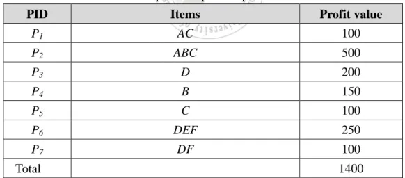
Table 2.1 shows an example of some products manufactured in a factory. There are seven items including A, B, C, D, E, F, and G, that we use to generate products. For example, P1 is

made from A and C, and the factory gains 100 dollars by producing it.

Table 2.1: A simple example of a product dataset

PID Items Profit value

P1 AC 100 P2 ABC 500 P3 D 200 P4 B 150 P5 C 100 P6 DEF 250 P7 DF 100 Total 1400

Let I = {i1, i2… im} be a set of m items, which represents the components for different

kinds of products in a factory. For a product subset X, X ⊆ I, the gain of X is defined as:

G(X) = ∑_{(𝑃𝑘|𝑋∩𝑃𝑘 .𝐼𝑡𝑒𝑚𝑠≠∅)}𝑃_𝐾. 𝑉𝑎𝑙. (1)

The gain of the itemset X is the sum of the profits of the products which include at least one item in X. For example, assume X = {A, B, C}. From Table 2.1, the four products P1, P2,

P4 and P5 include item A or B or C. Therefore, g(X) = P1.val

+

P2.val

+

P4.val

+

P5.val,

which is 850 (dollars). The definition of the total gain T is defined as:

T = ∑_{𝑃𝑘 ∈𝐷𝐵} 𝑃_𝑘. 𝑣𝑎𝑙. (2)

An itemset X is called an erasable itemsets if G(X) ≤ T × r, where r is a given threshold. For example, in Table 2.1, with r = 50%, we want to know whether the item B is erasable or not. Since B appears in P2 and P4, we can obtain its gain as 500 + 150, which is 650. T is 1400

in Table 2.1. The threshold gain is 1400 × 0.5 (50%), which is 700. In this process, we can know 700 > 650, so B is an erasable itemset. Above is a 1-itemset. For the 3-itemset {A, B,

C}, since A or B or C appears in P1, P2, P4 and P5, we can calculate its gain as 850 because

850 > 700 (threshold). So, {A, B, C} is a non-erasable itemset. The goal of the erasable-itemset mining is to find all the erasable itemsets from a product database with an erasable ratio parameter r [2].

2.2 Pre-Large Itemset Mining

In 2001, Hong et al. proposed the pre-large itemset mining [12][15] for maintaining frequent itemsets in dynamic environments. The pre-large mining algorithm [12][15] was used to solve the condition that wastes time to rescan original products with the FUP [5] algorithm. There are two parameters Sd and Su. Sd is the threshold of the lower bound and Su

is the threshold of the upper bound, which can divide all the itemsets into three parts. The itemsets lying between Sd and Su are called pre-large itemsets. Both the original transactions

and the new transactions thus have three kinds of itemsets: large itemsets, pre-large itemsets, and small itemset. One itemset is thus in one of the nine combinations. Each combination (case) is then processed in its own way to save the maintenance time.

2.3 Survey of Erasable Itemset Mining Algorithms

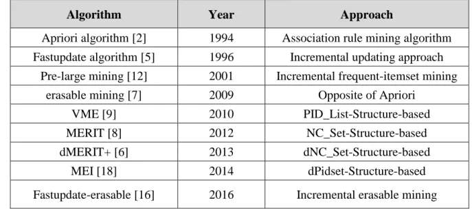
There were some proposed approaches related to erasable-itemset mining. Agrawal et al. proposed the apriori algorithm in 1994. Cheung et al. proposed the fastupdate algorithm in 1996. Deng et al. proposed the mining erasable (Meta) itemset algorithm in 2009. Deng and Xu proposed the vertical-format based (VME) algorithm for erasable-itemset mining in 2010. Deng and Xu proposed the MERIT algorithm, which was based on the concept of a tree data structure for fast mining erasable itemsets. Le et al. introduced a revised algorithm called dMERIT+, which came from MERIT to mine erasable itemsets with some pruning techniques. Le and Vo introduced an effective algorithm called mining erasable itemsets (MEI), which used a divide-and-conquer strategy and the concept of different PID_sets and the dPidset strategy of MEI to improve mining efficiency. Hong et al. proposed the fastupdate-erasable mining in 2016. Table 2.2 displays a summary of some existing algorithms for mining erasable itemsets.

Table 2.2: The history of existing algorithms for mining erasable itemsets

Algorithm Year Approach

Apriori algorithm [2] 1994 Association rule mining algorithm Fastupdate algorithm [5] 1996 Incremental updating approach

Pre-large mining [12] 2001 Incremental frequent-itemset mining

erasable mining [7] 2009 Opposite of Apriori

VME [9] 2010 PID_List-Structure-based

MERIT [8] 2012 NC_Set-Structure-based

dMERIT+ [6] 2013 dNC_Set-Structure-based

MEI [18] 2014 dPidset-Structure-based

Chapter 3

The Incremental Algorithm for Mining

ε-quasi-Erasable Itemsets

In this chapter, the Fastupdate-erasable approach[17] will be improved by the proposed algorithm. The algorithm’s main idea is described in Section 3.1; The notation used is described in Section 3.2; The new algorithm is proposed in Section 3.3. Finally, an example is given to explain the new algorithm in Section 3.4.

3.1 Main idea

If an itemset is non-erasable in an old database, but is erasable in the new products, then the old database needs to be re-scanned to determine whether it is erasable or not. However, if the gain of an itemset in an old database is much larger than the maximum erasable gain threshold, then it is hard for the itemset to become erasable even when some new products come. Figure 3.1 shows the concept behind the solution.

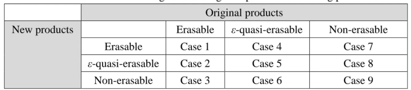
Table 3.1 Nine cases arising from adding new products to existing products Original products

New products Erasable ε-quasi-erasable Non-erasable

Erasable Case 1 Case 4 Case 7

ε-quasi-erasable Case 2 Case 5 Case 8

Non-erasable Case 3 Case 6 Case 9

Table 3.1 shows the nine cases arising from adding new products to existing products. When the itemset is erasable in the original products and the new products, which is case 1. When the itemset is erasable in the original products and the itemset is ε-quasi-erasable in the new products, which is case 2. When the itemset is erasable in the original products and the itemset is non-erasable in the new products, which is case 3. When the itemset is

ε-quasi-erasable in the original products and the itemset is erasable in the new products,

where is case 4. When the itemset is ε-quasi-erasable in the original products and the itemset is ε-quasi-erasable in the new products, which is case 5. When the itemset is ε-quasi-erasable in the original products and the itemset is non-erasable in the new products, which is case 6. When the itemset is non-erasable in the original products and the itemset is erasable in the new products, which is case 7. When the itemset is non-erasable in the original products and the itemset is ε-quasi-erasable in the new products, which is case 8. When the itemset is non-erasable in the original products and the itemset is non-erasable in the new products, which is case 9.

In the proposed algorithm, TP and TN represent the number of original products and number of new products. We give two parameters, r and ε, r be the maximum erasable ratio, and ε be the quasi-erasable parameter, if TN ≤ TP × (ε / r). The non-erasable-itemsets in original products cannot be erasable after inserting new products.

As mentioned above, if the total gain values of new products are small when compared to the total gain values of products in the original product database, then an itemset that is

neither erasable nor ε-quasi-erasable in the original database but is erasable in the newly inserted products cannot possibly be erasable for the entire updated product database. This property is proven in the following theorem.

Theorem: Let r be the maximum erasable ratio threshold and ε be the parameter value for

ε-quasi-erasable itemsets. Also, let 𝑇𝑃 _{and 𝑇}𝑁 _{be the total gain values of the items in the}

original products and in the new products, respectively. If 𝑇𝑁 ≤ 𝑇𝑃×𝜀_𝑟 , then an itemset

that is neither erasable nor ε-quasi-erasable in the original database but is erasable in the newly inserted products is certainly not erasable for the entire updated product database.

Proof: If 𝑇𝑁 ≤ 𝑇𝑃 ×𝜀_𝑟 is true, then the following derivation can be obtained:

𝑇𝑁 _{≤ 𝑇}𝑃_×𝜀 𝑟

 r × 𝑇𝑁_{≤ 𝑇}𝑃 _{× 𝜀}

If an itemset I is neither erasable nor ε-quasi-erasable in the original product database, its gain value gainP(I) in the original product database will satisfy the following inequality:

TP × (r + ε) < gainP(I)

If I is erasable in the newly inserted products, its gain value gainN(I) in the new products

will satisfy the following inequality:

0 ≤ gainN(I) ≤ TN × r

If the above three conditions are valid as stated in the theorem, then the entire gain value ratio of I in the updated product database U is 𝑔𝑎𝑖𝑛

𝑈_(𝐼)

𝑇𝑃_{+ 𝑇} 𝑁

,

which can be further expanded as

𝑔𝑎𝑖𝑛𝑈(𝐼) 𝑇𝑃_{+ 𝑇} 𝑁

=

𝑔𝑎𝑖𝑛𝑃(𝐼)+ 𝑔𝑎𝑖𝑛𝑁(𝐼) 𝑇𝑃_{+ 𝑇}𝑁

>

𝑇 𝑃_{× (𝑟 + 𝜀) + 0} 𝑇𝑃_{+ 𝑇}𝑁

=

𝑇 𝑃_{× (𝑟 + 𝜀)} 𝑇𝑃_{+ 𝑇}𝑁

=

(𝑇 𝑃_{× 𝑟) + (𝑇}𝑃_{× 𝜀)} 𝑇𝑃_{+ 𝑇}𝑁

≥

(𝑇 𝑃_{× 𝑟) + (𝑇}𝑁_{× 𝑟)} 𝑇𝑃_{+ 𝑇}𝑁

∵ (𝑇𝑃× 𝜀 ≥ 𝑇𝑁 × 𝑟)

=

𝑟 × (𝑇 𝑃 _{+ 𝑇}𝑁₎ 𝑇𝑃_{+ 𝑇}𝑁

= r

Thus: 𝑔𝑎𝑖𝑛 𝑈_(𝐼) 𝑇𝑃_{+ 𝑇} 𝑁

> r

So, I is not erasable. This completes the proof.

Therefore, when an itemset is neither erasable nor ε-quasi-erasable in the original products but is erasable in the newly inserted products, it is certainly not erasable for the entire updated product database when 𝑇𝑁 ≤ 𝑇𝑃×𝜀_𝑟 .

For example, assume 𝑇𝑃 = 1950, r = 35% and ε = 5%. The allowed total gain of new

products within which the original product database doesn’t need to be scanned is 1950 × (0.05 / 0.35), which is 278.57. It means if the gain of newly inserted products is equal to or smaller than 278.57, then an originally non-erasable itemset will certainly be still non-erasable without the need to rescan the old product database.

3.2 The Notations

used in this thesis are shown as follows:

P: the original products,

N: the set of newly inserted products, I: the set of all items,

U: the updated products, s: an itemset formed from I, gain: the gain value of an itemset,

gainP(s): the gain value of an itemset s in the original products P, gainN(s): the gain value of an itemset s in the new products N,

gainU(s): the gain value of an itemset s in the updated products U,

TP: the total gain value of all products in the original products P,

TN: the total gain value of all products in the set of newly inserted products N,

r: the maximum ratio to be an erasable itemset, ε: the quasi-erasable parameter,

EP: the set of erasable itemsets in the original products P,

EPk: the set of erasable k-itemsets in the original products P,

ENk: the set of erasable k-itemsets in the set of newly inserted products N,

EUk: the set of erasable k-itemsets in the updated products U,

QP: the set of ε-quasi-erasable itemsets in the original products P,

QPk: the set of ε-quasi-erasable k-itemsets in the original products P,

QNk: the set of ε-quasi-erasable k-itemsets in the set of newly inserted products N,

QUk: the set of ε-quasi-erasable k-itemsets in the updated products U,

CPk: the set of candidate itemsets from the original products P,

CNk: the set of candidate itemsets in the set of newly inserted products N,

3.3 The Proposed Incremental ε-quasi-erasable Itemset

Mining Algorithm

Based on the above idea, a ε-erasable-itemset mining algorithm can be designed. When a set of new products comes, the proposed algorithm will re-calculate the gain of an erasable itemset or a non-erasable itemset according to different cases, and decide whether the itemset is erasable. There are nine cases in total, by combining old product database and new products (each has three parts). A variable, t, is used to record the amount of gain from new products since the last re-scan of the original product database. The proposed algorithm is stated as follows:

The proposed algorithm:

Input: An original product P with its total profit value T

P

, the set of erasable itemsets EP and ε-quasi-erasable itemsets QP with their gain values from P plus previous new products since last re-scan, the amount of gain t from previous new products since the last re-scan, an erasable ratio threshold r, a quasi-erasable parameter ε, a set of all items I, and a set of newly coming products N.

Output: The set of erasable itemsets for the updated products U.

Step 1:

Calculate the safety gain f of new products as follows:

f = TP

×

𝜀_𝑟

(3)

Step 2:

Calculate the total profit value TN of the new products N as follows:

where Pi is a product in N. Then list the 1-itemsets appearing in the new products N

as the candidate erasable 1-itemsets and calculate their gain values from the new products N.

Step 3:

Set k = 1, where k records the number of items in the itemsets currently being processed.

Step 4:

Set 𝐶P

k = I − 𝐶Nk, where 𝐶Pk records the candidate k-itemsets not appearing in new

products.

Step 5:

Put a candidate erasable k-itemsets in into the set (CNk) of erasable k-itemsets for the

new products N if its gain value in the new products is smaller than or equal to the maximum gain threshold TN

×

r. Otherwise, put s into the set (QNk) of

ε-quasi-erasable k-itemsets for the new products N if its gain value in the new

products is larger than the maximum gain threshold TN

×

r but smaller than or equal to TN

×

(r

+

ε).

Step 6:

For each k-itemset s in the set of erasable k-itemsets (EPk) from the original products

P plus previous new products since last re-scan, if it is also in ENk, do the following

substeps (case 1):

Substep 6-1:

Set the updated gain of s as:

gainU(s) = gainP(s)

+

gainN(s),

where gainU(s), gainP(s), gainN(s) are the gains of s in the updated

product dataset, the original product dataset plus previous new products since last re-scan, and the set of current new products, respectively.

Substep 6-2:

Directly put s into updated erasable k-itemsets, EUk.

Step 7:

For each k-itemset s in the set of erasable k-itemsets (EPk) from the original products

P plus previous new products since last re-scan, if it is also in the candidate

(cases 2 and 3):

Substep 7-1:

Set the updated gain of s as:

gainU(s) = gainP(s)

+

gainN(s).

Substep 7-2:

Check whether the updated gain of s is smaller than or equal to the maximum erasable gain threshold (TP + TN)

×

r. If s satisfies the condition, put it in the set of updated erasable k-itemsets, EUk;

Otherwise, Check whether the updated gain of s is smaller than or equal to the maximumε-quasi-erasable gain threshold (TP

+

TN)

×

(r

+

ε). If s satisfies the condition, put it into updated

ε-quasi-erasable k-itemsets, QU k .

Step 8:

For the other k-itemsets in the set of erasable k-itemsets (EPk) from the original

products P plus previous new products since last re-scan, directly keep them in the set of updated erasable k-itemsets, EUk, with their gain values unchanged.

Step 9:

For each k-itemset s in the set of ε-quasi-erasable k-itemsets (QPk) from the original

product database P plus previous new products since last re-scan, if it is also in ENk,

do the following substeps (case 4):

Substep 9-1:

Set the updated gain of s as:

gainU(s) = gainP(s)

+

gainN(s),

where gainU(s), gainP(s), gainN(s) are the gains of s in the updated

products dataset, the original product dataset plus previous new products since last re-scan, and the set of current new products, respectively.

Substep 9-2:

Check whether the updated gain of s is smaller than or equal to the maximum erasable gain threshold (TP

+

TN)

×

r. If s satisfies the condition, put it in the set of updated erasable k-itemsets, EUk;

QUk ;

Step 10:

For each k-itemset s in the set of ε-quasi-erasable k-itemsets (QPk) from the

original products P plus previous products since last re-scan, if it is also in QNk,

do the following substeps (case5):

Substep 10-1:

Set the updated gain of s as:

gainU(s) = gainP(s)

+

gainN(s),

where gainU(s), gainP(s), gainN(s) are the gains of s in the updated

product dataset, the original product dataset plus previous new products since last re-scan, and the set of current new products, respectively.

Substep10-2:

Directly put s into updated ε-quasi-erasable k-itemsets, QUk.

Step 11:

For each k-itemset s in the set of ε-quasi-erasable k-itemsets (QPk) from the

original products P plus previous products since last re-scan, if it is also in the candidate erasable k-itemsets CNk but not in ENk and not in QNk (i.e. CNk − ENk

− QN

k), do the following substeps (case 6):

Substep 11-1:

Set the updated gain of s as:

gainU(s) = gainP(s)

+

gainN(s).

Substep 11-2:

Check whether the updated gain of s is smaller than or equal to the maximum ε-quasi-erasable gain threshold (TP

+

TN)

×

(r

+

ε). If s satisfies the condition, put it into ε-quasi-erasable k-itemsets, QNk.

Step 12:

For each s of the other k-itemsets in the set of ε-quasi-erasable k-itemsets (QNk)

from the original product database P plus previous new products since last re-scan, check whether the original gain, gainP(s), of s is smaller than or equal to the

maximum erasable gain threshold (TP

+

TN)

×

r. If s satisfies the condition, put it in the set of updated erasable k-itemsets, EU, with their gain values

unchanged; Otherwise, directly put it in the set of updated ε-quasi-erasable

k-itemsets, QUk, with their gain values unchanged.

Step 13:

For each k-itemset s which exists in (ENk

+

QNk − EPk − QPk) (erasable or

ε-quasi- erasable for new products, but not erasable nor ε-quasi-erasable for the original product database plus previous new products since last re-scan) or in CPk

− EP

k − QPk, put s into R (cases 7 and 8).

Step 14: If T

N

+

t ≤ f, then do nothing; Otherwise, do the following substeps for each k-itemset s in the rescan set R (cases 7 and 8):

Substep 14-1:

Rescan the original product database to determine gainP(s).

Substep 14-2:

If s is in (ENk

+

QNk − EPk − QPk), set the updated gain of s as:

gainU(s) = gainP(s)

+

gainN(s);

Otherwise, directly set the updated gain of s as:

gainU(s) = gainP(s)

Substep 14-3:

If the updated gain, gainU(s), of s is smaller than or equal to the

maximum gain threshold (TP

+

TN)

×

r, put s into updated erasable k-itemsets, EUk; Else if gainU(s) is smaller than or equal

to the maximum ε-quasi-erasable gain threshold (TP

+

TN)

×

(r

+

ε), put s into updated ε-quasi-erasable k-itemsets, QUk;

Otherwise, remove s from erasable k-itemsets (ENk) and from the

set of ε-quasi-erasable k-itemsets (QNk) from the new products.

Step 15:

Form the candidate erasable (k

+

1)-itemsets CUk+1 from the k-itemsets in EUk and

in QUk in a way similar to that in the batch algorithm. If a candidate erasable

(k

+

1)-itemsets generated includes at least one item in the new products, put s in

CNk+1 and calculate its gain value from the new products N. else put s in CPk+1.

Step 16:

Set k = k

+

1.

Step 17:

Repeat Steps 4-16 until no new candidate erasable itemsets are generated.

Step 19:

Output all the updated erasable itemsets.

3.4 An Example

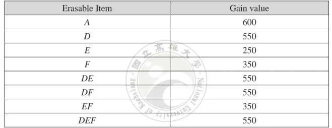
In this part, we will give an example to illustrate the process of algorithm, as we know, there are two products that will be inserted in original products, the threshold r is 0.45,

looking at the details below:

Table 3.2: The erasable itemsets found from Table 2.1

Erasable Item Gain value

A 600 D 550 E 250 F 350 DE 550 DF 550 EF 350 DEF 550

Table.3.3: Two newly inserted products in the example

PID Items Profit Value

P9 BE 100

P10 AC 150

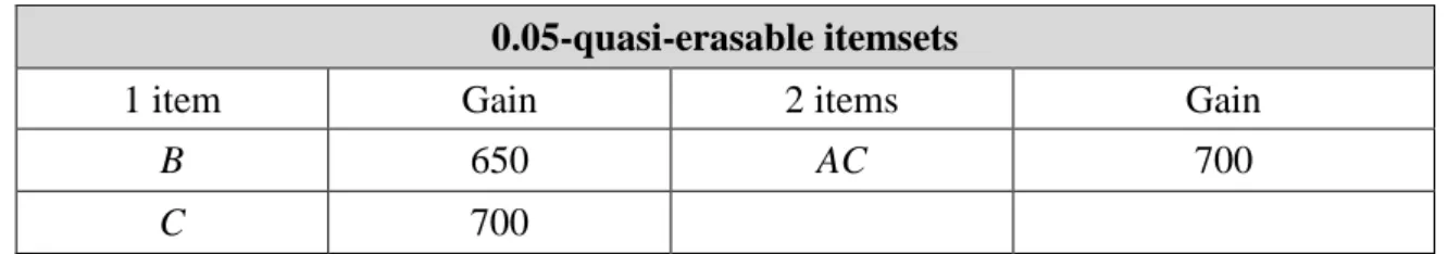
Assume the ε-quasi-erasable parameter ε is set at 0.05. The maximum gain threshold value for ε-erasable-itemsets is then calculated as the total gain multiplied by (r

+

ε), which is 1400

×

0.5 (= 700). The set of 0.05-quasi-erasable itemsets derived from the original products given in Table 3.4.

0.05-quasi-erasable itemsets

1 item Gain 2 items Gain

B 650 AC 700

C 700

Initially, the amount of gain t from the previous new products since the last re-scan of the original product database is zero. The ε-quasi-erasable mining algorithm then proceeds as follows.

Step 1: The gain f of new products for not re-scanning the original product database is

calculated, which is 1400

×

(0.05 / 0.45) (= 155.56).

Step 2:

The total profit value (TN) of the two new products given in Table 3.3 is first calculated as 100

+

150, which is 250. The 1-itemsets in the two new products are then listed as the candidate erasable 1-itemsets. They are A, B ,C and E, which appear in P9 and P10.

Their gain values in the new products are then calculated as (A: 150, B: 100, C: 150, E: 100). The results are shown in Table 3.5.

Table 3.5: The gain values of the four 1-itemsets in new products

1-itemset Gain value

A 150

B 100

C 150

E 100

Step 3:

The variable k is set at 1, where k records the number of items in the itemsets currently being processed.

Step 4:

CPk is then set as I – CNk, where I is the set of all items and records the candidate

1-itemsets not appearing in new products. In the example, I = {A, B, C, D, E, F} and CNk = {A,

Step 5:

The candidate erasable 1-itemsets in are checked for whether their gain values in the new products are smaller than or equal to the maximum gain threshold TN

×

r, which is

250 × 0.45 (= 112.5), or larger than the maximum gain threshold TN

×

r but smaller than or

equal to TN

×

(r

+

ε), which is 250

×

(0.45

+

0.05) (=125). In this example, no candidate erasable 1-itemsets satisfy the second condition, and thus the erasable 1-itemsets in is {B} and {E}, which satisfy the first condition.

Step 6:

For each 1-itemset in the set of erasable itemsets EP1 from the original product

database plus previous new products since last re-scan, if it is also in EN1, it is processed by

the substeps in this step. In this example, since is null from Step 5, there is no erasable 1-itemset in EP1 satisfies the condition.

Step 7:

Each candidate 1-itemset simultaneous existing in the set of erasable itemsets from the original product database plus previous new products since last re-scan and in CNk –

ENk is processed. In this example, only the 1-itemset {A} satisfies the condition. The gain

value of {A} in the original database is 600 and in the new products is 150. The updated gain value of {A} is then calculated as 600 + 150, which is 750. The value is then compared to the gain threshold, which is (TP

+

TN)

×

r (= 742.5) and (TP

+

TN)

×

(r

+

ε) (= 825).

Since the updated gain value (750) of the 1-itemset {A} is bigger than 742.5, and that is smaller than 750. So, {A} is not an erasable 1-itemset but is a ε-quasi-erasable 1-itemset.

Step 8:

The remaining 1-itemsets not processed in the set of erasable k-itemsets (EPk)

from the original product database plus previous new products since last re-scan are {D}, {E} and {F}. They are then directly put into the set of updated erasable 1-itemsets, EU1, with their

gain values unchanged.

Step 9:

For each k-itemset s in the set of ε-quasi-erasable k-itemsets (QPk) from the

original product database P plus previous new products since last re-scan, if it is also in ENk,

0.5. Finally, the {B} is a ε-quasi-erasable 1-itemset.

Step 10:

For each k-itemset s in the set ofε-quasi-erasable k-itemsets (QPk) from the

original product database P plus previous new products since last re-scan, if it is also in QNk,

it is then processed in this step. In this example, no itemset satisfies the condition.

Step 11:

For each k-itemset s in the set ofε-quasi-erasable k-itemsets (QPk) from the

original product database P plus previous new products since last re-scan, if it is also in the candidate erasable k-itemsets but not in ENk and not in QNk (i.e. CNk − ENk − QNk), it is

processed in this step. In this example, {C} satisfies the condition. The gain value of {C} is the calculated as 700

+

150 (= 850), which compared with 1650

×

0.45 and 1650

×

0.5. Finally, the {C} satisfies neither first condition nor second condition.

Step 12:

There are no other 1-itemsets in the set of ε-quasi-erasable k-itemsets (QPk)

from the original product database P plus previous new products since last re-scan. Nothing is done.

Step 13:

For each 1-itemset s which exists in (EN1

+

QN1 − EP1 − QP1) (erasable orε

-quasi- erasable for new products, but not erasable norε-quasi-erasable for the original product database plus previous new products since last re-scan) or in CP1 − EP1 − QP1 , put

s in the rescan set R. In this example, not only no itemsets exists in (CP1 − EP1 − QP1) but

also no itemsets exist in EN1

+

QN1 − EP1 − QP1.

Step 14:

TN

+

t = 250 + 0 = 250. Although it is bigger than f (≈ 155.56), not only no

itemsets exists in (CP1 − EP1 − QP1) but also no itemsets exist in EN1

+

QN1 − EP1 − QP1.

So, this step should not be processed.

Step 15:

The candidate erasable 2-itemsets CU2 are then formed from the 1-itemsets in

EU1 and in QU1. In this example, and includes the five 1-itemsets: {A}, {D}, {E}, and {F}.

The following six candidate 2-itemsets are then generated: {AD}, {AE}, {AF}, {DE}, {DF}, {EF}. They are then partitioned into two parts, CN2 and CP2, depending on whether at least

one item in the new products are included. The results of CN2 with gain values from the two

new products are shown in Table 3.6. Besides, CP2 contains {DF}.

Table 3.6: The gain values of the erasable 2-itemsets in CN2

2-itemset Gain Value from N

AD 150

AE 250

AF 150

DE 100

EF 100

Step 16:

The variable k is increased as 2.

Step 17:

In this example, since ten candidate erasable itemsets are generated in Step 15, Steps 5 to 11 are repeated as follows. In Step 5, {DE}, {EF} are then put into the erasable 2-itemsets for the new products since their gains are smaller than or equal to TN

+

r, which is 112.5. No candidate put into the ε-quasi-erasable 2-itemsets for the new products since their gains are smaller than or equal to TN

×

(r

+

ε), which is 125. The results of with gain values from the two new products are shown in Table 3.7.

Table 3.7: The gain values of the ε-quasi-erasable 2-itemsets in EN2

2-itemset Gain value from N

DE 100

EF 100

{DE} and {EF} itemsets satisfy the condition in Step 6. Their updated gain values are calculated as 550+100, 550+100, which are all smaller than (TP

+

TN)

×

r, so, we put them into EU2. No itemsets satisfy the condition in Step 7. Then in Step 8, the remaining one

{AD}, {AE} and {AF} are in CN2 − EN2 − QN2 and are thus processed. Their updated gain

values are calculated as 1150

+

150, 850

+

250 and 950

+

150, which are all larger than (TP

+

TN)

×

(r

+

ε). They are then ignored. Step 12 There is {AC} 2-itemset in QP2. {AC}

can be calculated as 700

+

150, which is larger than (TP

+

TN)

×

(r

+

ε). In Step 13, no

2-itemset in (EN2

+

QN2 − EP2 − QP2) and no 2-itemset is in (CP2 − EP2 − QP2).

After Step 14, EU2 includes {DE}, {DF} and {EF}, and no itemset in QU2. Then in Step

15, the only candidate erasable 3-itemset, {DEF}, is generated. It is put into CN3. CP3 is null.

The variable k then becomes 3 and Steps 5 to 16 are executed again. The only 3-itemset, {DEF}, is processed in Step 6 and is directly put into the updated erasable 3-itemset EU3.

There are no new candidate 4-itemsets generated and Step 18 is executed.

Step 18:

Since TN

+

t ≥ f, t = 0.

Step 19:

All the updated erasable itemsets generated so far are output to users. The results are shown in Table 3.8.

Table 3.8: The final updated erasable itemsets Erasable itemsets

1-itemset Gain 2-itemsets Gain 3-itemsets Gain

D 550 DE 650 DEF 650

E 350 DF 550

F 350 EF 450

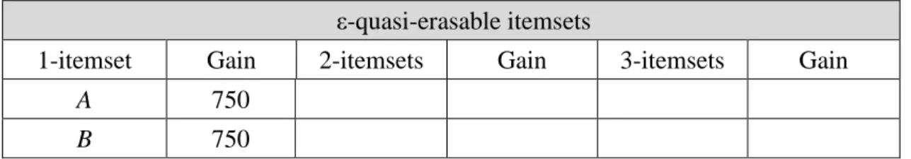
Note that after the two new products are processed, t = 250, and the ε-quasi-erasable itemsets are shown in Table 3.9.

Table 3.9: The final updated ε-quasi-erasable itemsets ε-quasi-erasable itemsets

1-itemset Gain 2-itemsets Gain 3-itemsets Gain

A 750

B 750

confirmed as erasable, ε-quasi-erasable or not ε-quasi-erasable in Step 14 only when TN

+

t > f. When TN

+

t ≤ f, they cannot be erasable according to the derived theorem.

Chapter 4

Experiments and Analysis

4.1 Experimental Environment and Data Sets

We conducted experiments to show the performance of the proposed algorithm. The other two approaches, meta-erasable [7] and fastupdate-erasable [16], were also compared. Experiments were implemented in Java and executed on a notebook with a 2.5 GHz CPU and 12GB of memory. The way to generate the dataset is described as follows.

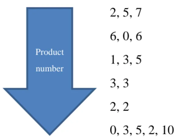
Assume we wanted to generate N products, each of which consisted of some material items. The length of material items for each product was first randomly generated within 1 to a given maximum length L. After the length of a product was generated, each item ID within 0 to I was generated randomly, where I

+

1 is the total number of material items in the whole database. Note that the first item ID was 0 in the dataset and a same item ID could not be generated twice for a product. The profit of a product was then set as the sum of the ID values of the items in the product. For example in Figure 4.1, six products are generated. The first product is (2, 5, 7), in which the first two numbers, 2 and 5, represent the item IDs and the last number, 7, represents the profit of the product. The profit is decided by 2

+

5 in this dataset.

Figure 4.1: The way to generating a product base

4.2 Experimental Results

The experimental result for the datasets is shown in this section.

Experiments were conducted for the dataset generated by the random program. Table 4.1 shows the parameter setting.

Table 4.1: The parameter setting on the dataset

Parameter Value Description

r 0.5 The maximum erasable threshold

ε 0.05 The quasi-erasable parameter

P 100000 The number of original products

N 1000, 5000 The two numbers of newly inserted products

I 20 The number of items

length 4 The maximum number of items in each product

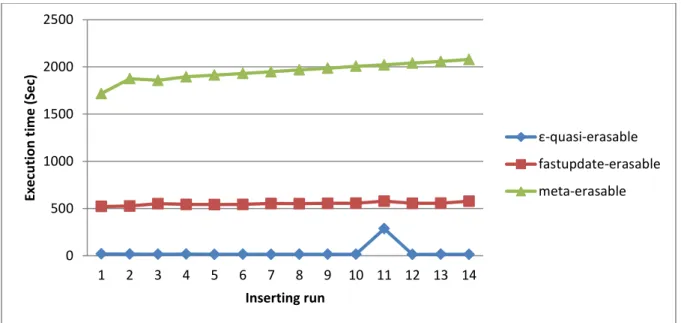
The following three algorithms are compared: ε-quasi-erasable mining, fastupdate-erasable mining [16], and meta-erasable mining [7]. Each time, 1000 new products were inserted and merged into the original product database. Figure 4.2 shows the execution

2, 5, 7

6, 0, 6

1, 3, 5

3, 3

2, 2

0, 3, 5, 2, 10

Product number

time of the three algorithms. The y-axis represents the execution time, whose units are in seconds, and the x-axis denotes the inserting runs.

Figure 4.2: The execution time of the three algorithms for N = 1000

In Figure 4.2, the proposed ε-quasi-erasable mining algorithm was the fastest among the three, the fastupdate-erasable was the second fastest, and the meta-erasable was the slowest. The reason was the ε-quasi-erasable mining algorithm did not need to scan the product database in the first several runs because the accumulated gain value of the new products had not yet gotten to the allowed gain value, which was calculated from the formula in Section 3.1. In the eleventh run, the execution time rose abruptly because the accumulated gain value of the new products had exceeded the allowed gain value and the old product database needed to be rescanned, which took a lot of time. But even in this case, its execution time at the run was still not larger than that by the fastupdate-erasable algorithm. After the run, the accumulated gain value was reset and the execution time became little again. Compared to the ε-quasi-erasable algorithm, the fastupdate-erasable algorithm always needed to rescan the product database for the itemsets that were non-erasable in the original product database but erasable in the new products. The fastupdate-erasable mining algorithm was slower than the

0 500 1000 1500 2000 2500 1 2 3 4 5 6 7 8 9 10 11 12 13 14 Exec u tion t im e ( Se c) Inserting run ε-quasi-erasable fastupdate-erasable meta-erasable

ε-quasi-erasable mining algorithm. It could, however, save the rescanning time for the other

cases. Thus, it was faster than the meta-erasable mining algorithm.

Figure 4.3 shows the numbers of erasable itemsets and ε-quasi-erasable itemsets. The y-axis represents the number of itemsets and the x-axis denotes the inserting run. Note that all the three algorithms had the same erasable itemsets, and only the proposed algorithm needed to keep the ε-quasi-erasable itemsets, which were the overhead of the algorithm for fast execution. In this experiment, the number of erasable itemsets was about 250, and the number of ε-quasi-erasable itemsets was about 100, which was small when compared to 250. It is noteworthy that to keep the additional ε-quasi-erasable itemsets for significantly saving execution time. Additionally, the numbers of erasable itemsets in the runs were about the same because a small number of new products would not affect the whole product database much.

Figure 4.3: The numbers of erasable and ε-quasi-erasable itemsets obtained by the proposed algorithm for N= 1000

Experiments were then conducted for inserting 5000 new products each time. Except the number of newly inserted products, the other parameters were set at the same values as those

0 50 100 150 200 250 300 1 2 3 4 5 6 7 8 9 10 11 12 13 14 N u m b e r o f i te m set s Inserting run erasable itemsets ε-quasi-erasable itemsets

gain value was reached for about every three runs.

Figure 4.4: The execution time of the three algorithms for N = 5000

Comparing Figures 4.2 and 4.4, it was found that the experiments for N = 5000 had a higher frequency of peak time than those for N = 1000. This phenomenon could be easily validated by the theorem proposed previously. Additionally, the peak time increased along with the inserted run number because the size of the original product database increased after each run.

Figure 4.5 then shows the numbers of erasable and ε-quasi-erasable itemsets for inserting 5000 products. Like the results in Figure 4.3, the number of ε-quasi-erasable itemsets was much smaller than that of erasable itemsets if the quasi-erasable parameter ε was small.

0 500 1000 1500 2000 2500 3000 3500 1 2 3 4 5 6 7 8 9 10 11 12 13 14 Exec u tion t im e ( Se c) Inserting run ε-quasi-erasable fastupdate-erasable meta-erasable

Figure 4.5: The numbers of erasable and ε-quasi-erasable itemsets obtained by the proposed algorithm for N = 5000

Next, experiments were conducted for different numbers of new products, including N = 1000, 3000, 5000, 7000 and 9000. The size of the original product database is 100000. Besides, r = 0.5 and ε = 0.05. Figure 4.6 shows the execution time of the first inserting run for different N values. In Figure 4.6, all the execution didn’t need to scan the original product database. 0 50 100 150 200 250 300 1 2 3 4 5 6 7 8 9 10 11 12 13 14 N u m b e r o f i te m set s Inserting run erasable itemsets ε-quasi-erasable itemsets 0 20 40 60 80 100 120 0 1000 2000 3000 4000 5000 6000 7000 8000 9000 10000 Exec u tio n t im e ( Se c)

It could be observed from Figure 4.6 that the more products were inserted, the more execution time was needed. The relationship between the number of new products and the execution time was nearly linear. The reason was that the ε-quasi-erasable mining algorithm needed to scan the new products. So, when more new products were processed, more execution time would be spent. The execution time would be proportional to the size of new products. Figure 4.7 shows the number of erasable and ε-quasi-erasable itemsets for different numbers of new products. It could be seen that nearly the same quantities of erasable and

ε-quasi-erasable itemsets were generated for the different numbers of new products.

Figure 4.7: The numbers of erasable and ε-quasi-erasable itemsets for different N values

Experiments were then made to show the effects of the original product database size. For inserting 1000 new products, the execution time for different sizes of original product databases was shown in Figure 4.8. The execution time was measured for the first inserting run, in which no rescan was needed.

0 50 100 150 200 250 300 1000 3000 5000 7000 9000 N u m b e r o f i te m set s

Number of new products

erasable itemsets

Figure 4.8: The execution time without rescanning for different sizes of original product databases.

It could be seen from Figure 4.8 that nearly the execution time was the same for different sizes of original product databases. This was because the above execution process didn’t need to rescan the original product databases but only needed to check the erasable and

ε-quasi-erasable itemsets. Since the numbers of erasable and ε-quasi-erasable itemsets are nearly the same, which are shown in Figure 4.9, thus the execution time is about equal as well. 0 2 4 6 8 10 12 14 16 18 20 0 50000 100000 150000 200000 250000 Exec u tion t im e ( Se c)

Figure 4.9: The numbers of erasable and ε-quasi-erasable itemsets without rescanning for different sizes of original product databases.

In Figure 4.9, the number of the ε-quasi-erasable itemsets was much smaller than that of the erasable itemsets when ε was small (ε = 0.05 in this case). Besides, different sizes of original product databases generated nearly the same numbers of erasable (and

ε-quasi-erasable) itemsets because the data distribution was about the same.

Next, experiments were conducted to measure the execution time with rescanning for different numbers of original products. When the original product database size was 25000, the rescanning occurred in the third inserting run. So, the x-value of the corresponding point was 27000. When the original product database size was 50000, the rescanning occurred in the sixth inserting run. So, the x-value of the corresponding point was 55000. At last, the original product database size was 100000, the rescanning occurred in the eleventh inserting run. So, the x-value of the corresponding point was 110000. The results are shown in Figure 4.10. 0 50 100 150 200 250 300 0 50000 100000 150000 200000 250000 N u m b e r o f i te m set s

Number of original products

erasable itemsets

Figure 4.10: The execution time with rescanning for different sizes of original product databases

Note that in Figure 4.10, the execution time was measured for the runs that needed rescanning. It could be observed from Figure 4.10 that the bigger the original product database size was, the more execution time was needed. The relationship between the size of the original product database and the execution time was nearly linear. The reason was that when rescanning was needed, the ε-quasi-erasable mining algorithm scanned the original databases to get the actual gain values of some candidates. So, when more original products were in the database, more execution time would be spent. The execution time would be proportional to the size of the original product database.

Figure 4.11 shows the number of erasable and ε-quasi-erasable itemsets with rescanning for different sizes of original product databases. The results were like those in Figure 4.9. The number of the ε-quasi-erasable itemsets was much smaller than that of the erasable itemsets when ε is small. Besides, different sizes of original product databases generated nearly the same numbers of erasable (and ε-quasi-erasable) itemsets because the data distribution was nearly the same.

0 50 100 150 200 250 300 350 0 25000 50000 75000 100000 Exec u tion t im e ( Se c)

Figure 4.11: The number of erasable and ε-quasi-erasable itemsets with rescanning for different sizes of original product databases

Next, experiments were conducted for different maximum erasable thresholds, including r = 10%, 30%, 50%, 70%, and 90%. The other parameter values were the same as those in Table 4.1. Figure 4.12 shows the numbers of erasable itemsets and ε-quasi-erasable itemsets for inserting the first 1000 new products.

Figure 4.12: The numbers of erasable itemsets and ε-quasi-erasable itemsets for different r values and ε = 0.05 0 50 100 150 200 250 300 0 25000 50000 75000 100000 N u m b e r o f i te m set s

Number of original products

erasable itemsets ε-quasi-erasable itemsets 0 2000 4000 6000 8000 10000 12000 14000 16000 18000 10% 30% 50% 70% 90% N u m b e r o f i te m set s

Maximum erasable threshold

erasable itemsets

It was observed from this figure that the bigger the threshold r was, the more erasable itemsets were generated. It could be easily known from the definition of erasable itemsets. The number of the ε-quasi-erasable itemsets depended on the dataset because the quasi-erasable parameter was fixed in Figure 4.12. Figure 4.13 shows the execution time of the ε-quasi-erasable mining algorithm with different thresholds.

Figure 4.13: The execution time of the proposed algorithm with different thresholds

The execution time increased along with the increase of the r value. The reason was more erasable itemsets would be generated when the threshold was bigger, causing more execution time.

Experiments were then conducted for different values of the quasi-erasable parameter ε. The numbers of erasable and ε-quasi-erasable itemsets for ε= 1%, 2%, 3%, 4%, 5%, 6%, 7%, 8%, 9%, and 10% are shown in Figure 4.14.

0 50 100 150 200 250 300 350 10% 30% 50% 70% 90% Exec u tion t im e ( Se c)

Figure 4.14: The numbers of erasable itemsets and ε-quasi-erasable itemsets of the proposed algorithm with different ε values and r = 0.5

In Figure 4.14, the bigger the ε value was, the more ε-quasi-erasable itemsets would be generated in the ε-quasi-erasable mining algorithm. It was reasonable because a bigger ε value would cause a larger range of ε-quasi-erasable itemsets. Note that the numbers of erasable itemsets for different ε values are the same since the threshold r is fixed at 0.5. The experimental results for comparing the execution time of different quasi-erasable parameter values are shown in Figure 4.15.

Figure 4.15: The execution time of the proposed algorithm with different ε and r = 0.5 0 100 200 300 400 500 600 1% 2% 3% 4% 5% 6% 7% 8% 9% 10% N u m b e r o f i te m set s Quasi-erasable parameter erasable itemsets ε-quasi-erasable itemsets 0 2 4 6 8 10 12 14 16 18 20 0% 1% 2% 3% 4% 5% 6% 7% 8% 9% 10% 11% 12% Exec u tion t im e ( Se c) Quasi-erasable parameter

In Figure 4.15, the execution time slightly increased along with the increase of the ε value. This was because when the ε value increased, more ε-quasi-erasable itemsets were generated, causing more checking time.

Experiments were then conducted for comparing the execution time of different numbers of items for I = 10, 15, 20, and 25. The results are shown in Figure 4.16.

Figure 4.16: The execution time of different numbers of itemsets with ε = 0.05 and r = 0.5

It was observed that the more items were used in manufacturing the products, the more execution time was spent. The reason for this was that both the erasable itemsets and the

ε-quasi-erasable itemsets would increase as the number of items increased. When more

candidate itemsets were generated, the corresponding execution time would become more as well. The numbers of erasable and ε-quasi-erasable itemsets for different numbers of items are shown in Figure 4.17.

0 10 20 30 40 50 60 70 80 0 5 10 15 20 25 30 Exec u tion t im e ( Se c) Number of items

Figure 4.17: The numbers of itemsets of number of itemsets with ε = 0.05 and r = 0.5

The numbers of erasable itemsets and ε-quasi-erasable itemsets might increase along with the increase of the items. The reason was that when more items existed, the possible combinations of itemsets would increase as well.

0 500 1000 1500 2000 2500 0 5 10 15 20 25 30 N u m b e r o f i te m set s Number of items erasable itemsets ε-quasi-erasable itemsets

Chapter 5

Conclusion and Future Work

In this thesis, we propose the concept of the ε-quasi-erasable itemsets and use it to improve the mining performance of erasable itemsets for dynamic environments. When the previous fastupdate-erasable algorithm handles its case 3, much time will be spent because the original product database needs to be rescanned. Therefore, we define ε-quasi-erasable itemsets to help accelerate the execution speed. We also prove the proposed approach can significantly reduce the rescanning number if the number of new products is small. To show the proposed mining algorithm is efficient, a lot of experiments are conducted. The results demonstrate that the proposed algorithm executes faster than both the META-erasable algorithm and the fastupdate-erasable algorithm in incremental mining for certain parameter settings. Experiments are finally made to verify the performance.

In the future, we will design the ε-quasi-erasable itemset mining for deletion and modification. In addition, we will also use different data structures like trees [11][22] to improve the efficiency.

References

[1] R. Agrawal, T. Imielinski and A. Swami, “Mining association rules between sets of items in large databases,” The ACM SIGMOD International Conference on Management of

Data, pp. 207–216, 1993.

[2] R. Agrawal and R. Srikant, “Fast algorithm for mining association rules,” The 20th

International Conference on Very Large Data Bases, pp. 487–499, 1994.

[3] K. R. Anil and R. S. Gladston, “N-list based friend recommendation system using pre-rule checking,” International Journal of Computer Science and Information Technologies, Vol. 7, pp. 338–341, 2016.

[4] K. Bharati and D. Kanchan, “Comparative study of frequent itemset mining algorithms: FP growth, FIN, prepost + and study of efficiency in terms of memory consumption, scalability and runtime,” International Journal of Technical Research and Applications, Vol. 4, Issue 6, pp. 72–77, 2016.

[5] D. W. Cheung, J. Han, V. T. Ng and C. Y. Wong, “Maintenance of discovered association rules in large databases: Agrawal approach,” The 12th IEEE International Conference on

Data Engineering, pp. 106–114, 1996.

[6] F. Coenen, T. Le and B. Vo, “An efficient algorithm for mining erasable itemsets using the difference of NC-Sets,” The IEEE International Conference on Systems, Man, and

Cybernetics Manchester, pp. 2270–2274, 2013.

[7] Z. H. Deng, G. D. Fang, Z. H. Wang and X. R. Xu, “Mining erasable itemsets,” The 8th

International Conference on Machine Learning and Cybernetics, pp. 12–15, 2009.

[8] Z. H. Deng and X. R. Xu, “Fast mining erasable itemsets using NC_sets,” Expert Systems

with Applications, Vol. 39, pp. 4453–4463, 2012.