A Hybrid Prototype Construction and Feature Selection Method with
Parameter Optimization for Support Vector Machine
Ching-Chang Wong and Chun-Liang Leu
Department of Electrical Engineering, Tamkang University, Tamsui, Taiwan, R.O.C.
E-mail: [email protected] , [email protected]
Abstract
-In this paper, an order-independent algorithm for data reduction, called the Dynamic Condensed Nearest Neighbor (DCNN) rule, is proposed to adaptively construct prototypes in training dataset and to reduce the over-fitting affect with superfluous instances for the Support Vector Machine (SVM). Furthermore, a hybrid model based on the genetic algorithm is proposed to optimize the prototype construction, feature selection, and the SVM kernel parameters setting simultaneously. Several UCI benchmark datasets are considered to compare the proposed GA-DCNN-SVM approach with the GA-based previously published method. The experimental results show that the proposed hybrid model outperforms the existing method and improves the classification accuracy for SVM.Keywords: dynamic condensed nearest neighbor,
prototype construction, feature selection, genetic algorithm, support vector machine.
1. Introduction
The support vector machine (SVM) was first proposed by Vapnik [1] and has been successful as a high performance classifier in several domains including data mining and the machine learning research community. Due to the data sets that we process today are becoming increasingly larger, not only in terms of the number of patterns (instances), but also the dimension of features (attributes), which may degrade the efficiency of most learning algorithms, especially when there exist redundant instances or irrelevant features. However, for some datasets, the performance of SVM is sensitive to how the kernel parameters are set [2]. As a result, obtaining the optimal essential instances, features subset and SVM parameters must occur simultaneously.
In the literature, several data reduction algorithms have been proposed that extract a consistent subset of the overall training set, namely, Condensed Nearest Neighbor (CNN), Modified CNN (MCNN), Fast CNN (FCNN), and others
[3-6], that is, a subset that correctly classifies all the discarded training set objects through the NN rule. These algorithms have been shown in some cases to achieve condensation ratios corresponding to a small percentage of the overall training set and to obtain the comparable classification accuracy. However, these papers solely focused on data reduction, but not deal with features selection to reduce the irrelevant features for the classifier. Feature selection algorithms may be widely categorized into two groups: the filter and the wrapper approaches [7-8]. The filter approaches select highly ranked features based on a statistical score as a preprocessing step. They are relatively computationally cheap since they do not involve the induction algorithm. Wrapper approaches, on the contrary, directly use the induction algorithm to evaluate the feature subsets. They generally outperform filter methods in terms of classification accuracy, but are computationally more intensive. Huang and Wang [2] proposed a GA-based feature selection method that optimized both the feature selection and parameters setting for the SVM classifier, but they did not take into account the treatment of these redundant or noisy instances in a classification process. So far, to the best of our knowledge, there is no other research using an evolutionary algorithm to simultaneously solve these three type problems as mentioned above.
In this paper, we first introduce a new data reduction algorithm which differs from the original CNN in its employments of the voting scheme for prototype construction and the adaptively merged rate for prototype augmentation. Hence, it is called the dynamic CNN (DCNN) algorithm. Second, we proposed a novel GA-DCNN-SVM model that hybridized the prototype construction, feature selection and parameters optimization methods with genetic algorithm, exhibiting high efficiency in terms of classification accuracy for SVM. The rest of this paper is organized as follows. Section 2 describes the related works including the basic SVM, the CNN rule and GA concepts. In section 3, the prototype voting scheme, the DCNN algorithm and the hybrid model are presented.
Section 4 contains the experimental results from using the proposed method to classify several UCI benchmark datasets and comparison with the GA-based previously published method. Finally, in section 5, conclusions are drawn.
2. Related works
2.1. SVM classifier
SVM starts from a linear classifier and searches the optimal hyperplane with maximal margin. Given a training set of instance-label pairs
( , ),x yi i i=1, 2,...,m where
n i
x∈R and yi∈ + −{ 1, 1} . The generalized linear SVM finds an optimal
separating hyperplane f x( )= w x⋅ + b by solving
the following optimization problem:
, , 1 1 Min 2 m T i w b i w w C ξ ξ = +
∑
Subject to: ( ) (1) 0 i i i i y w x b ξ ξ < ⋅ > + + − ≥ ≥ 1 0,where C is a penalty parameter on the training
error, andξiis the non-negative slack variables.
This optimization model can be solved using the Lagrangian method, a dual Lagrangian must be
maximized with respect to a non-negativeα under i
the constrains and , and the
optimal hyperplane parameters and can be
obtained. The optimal decision hyperplane
1 0 m i i i y α = =
∑
0≤αi≤C * w b* * * ( , , )f xα b can be written as:
* * * * * * 1 ( , , ) m i i i i f xα b yα x x b w x b = =
∑
< ⋅ > + = ⋅ + (2)Linear SVM can be generalized to non-linear
SVM via a mapping function , which is also
called the kernel function, and the training data can be linearly separated by applying the linear SVM formulation. The inner product
Φ
( ( )Φ xi ⋅ Φ( ))xj is
calculated by the kernel functionk x for given
training data. Radial basis function (RBF) is a common kernel function as Eq. (3). In order to improve classification accuracy, the kernel parameter
( , )i xj
γshould be properly set.
Radial Basis Function kernel:
(3)
2
( , ) exp(i j || i j|| )
k x x = −γ x −x 2.2. The CNN algorithm
The condensed nearest neighbor (CNN) rule first introduced by Hart [3] is that patterns in the training set may be very similar and some do not add extra information and thus may be discarded. The algorithm uses two bins, called training set S
and prototype subset P. Initially, randomly select one sample from S to P. Then, we pass one by one over the samples in S per epoch and classify each
patterxi∈Susing P as the prototype set. During
the scan, whenever a patternxiis misclassified, it is
transferred from S to P and the prototype subset is
augmented; otherwise the pattern xi is called
merged into P and still left in S. The algorithm terminates when no pattern is transferred during a complete pass of S and no new prototype is added to P. In other words, the CNN rule stops when all samples in S have been fully merged into these prototypes in P.
The CNN algorithm pseudo code is shown in Figure 1. This method, being a local search, does not guarantee finding the minimal subset and furthermore, different subsets are found when the process of training set order is changed.
Algorithm CNN rule
Input: A training set S;
Output: A prototype subset P; 1 Initiation
2 P: {}= ;
3 Randomly select a new prototype to P; 4 Repeat
5 Augmentation = False; 6 For all patterns x S∈ usingp*∈P 7 IF class x( )≠class p( )* Then
8 P:= ∪ ; P x
9 Augmentation = True; 10 End IF
11 End For
12 Until Not ( Augmentation ); 13 Return ( P );
Fig. 1. Pseudo code of the CNN algorithm.
2.3. Genetic algorithm
Genetic algorithm (GA) is one of the most effective approaches for solving optimization problem. The basic idea of GA is to encode candidate solutions of a problem into genotypes, and candidate solutions could be improved through the evolution mechanism, such as selection, crossover, and mutation.
The GA consists of six main steps: population initialization, fitness calculation, termination check, selection, crossover, and mutation. In the beginning, the initial population of a GA is generated randomly. Then, the evaluation values of the fitness function for the individuals in the current population are calculated. After that, the termination criterion is checked, and the whole GA procedure stops if the termination condition is satisfied. Otherwise, these operations of selection,
crossover, and mutation are performed.
3. Methods
We start by giving some preliminary definitions. Assume that we are given a dataset in which
{( , ),i i 1, 2,..., }
S= x y i= m is a set of m number of
samples with well-defined class labels. Note that is the vector of dataset for the
i-th sample describing in D-dimensional Euclidean
space and is the class label associated with
1 2 ( , ,..., )T i i i iD x = x x x i y xi,
, q is the number of classes.
1 2
{ , ,..., }
i
y∈ =C c c cq
Our goal is to extract a small consistent subset
P from S, whereP=
{
( , ),x yj j j=1, 2,...,n and n<m}
,such that p*∈P is the nearest pattern tox∈S.
Members of P are called prototypes. The distance
between any two vectors xi and x using the j
distance measured( )⋅ is:
1/ 2 2 1 ( , )i j i j D ( ik jk) k d x x x x x x = ⎡ = − =⎢ − ⎣
∑
⎦ ⎤ ⎥ (4)3.1. Prototype voting scheme (PVS)
Majority vote is one of the simplest and intuitive ensemble combination techniques. Consider the n samples, c-class dataset U from S, given an
instancexiof U, the nearest neighbors’ distance
vector (NNDV) ofxiin U according to a distance d:
,1, ,2, , , , 1, , , ( )i i c i c i j c i n c i n c , NNDV x = ⎣⎡d d L d L d − d ⎤⎦ (5) , , 1, ( , ) min ( , ) 0, ( , ) min ( , ) 1,2,..., , 1,2,..., . i j j i j i j c i j j i j d x x d x x and i j d d x x d x x or i j i n j n = ≠ ⎧⎪ = ⎨ ≠ = ⎪⎩ = = (6)
We pass one by one over all of the instances in
U, the outputs of NNDV in U are first organized
into a decision prototype matrix (DPM) as shown
in Figure 2. The column ford1, ,j cto represents
the support from samples
, ,
n j c d
1
x to xn for the
candidate point xj, and the row to is
the NNDV of
,1,
i c d di n c, ,
i
x. The vote will then result in an
ensemble decision for the candidate point xλ, and
the λ value is:
, , 1 1 arg maxn n i j c j i d λ = = =
∑
(7) The candidate point with the highest total support is then chosen as the prototype. The pseudo code of the prototype voting scheme (PVS) algorithm is shown in Figure 3.
1,2, 1, , 1, 1, 1, , 2,1, 2, , 2, 1, 2, , ,1, ,2, , , , 1, , , 1,1, 1,2, 1, , 1, , ,1, ,2, , , , 1, 0 0 0 0 c j c n c c j c n c i c i c i j c i n c i n c n c n c n j c n n c n c n c n j c n n c d d d d d d d d d d d d DPM d d d d d d d d − − − − − − − − n c n c d ⎡ ⎤ ⎢ ⎥ ⎢ ⎥ ⎢ ⎥ ⎢ ⎥ = ⎢ ⎥ ⎢ ⎥ ⎢ ⎥ ⎢ ⎥ ⎢ ⎥ ⎣ ⎦ L L L L M M O M N M M L L M M N M O M M L L L L
Fig. 2. Decision Prototype Matrix of the PVS.
Fig. 3. Pseudo code of the PVS algorithm Algorithm PVS rule
Input: A training set U with c-class from S;
Output: A prototype pointλ; 1 For all patternsxiin U
2 For each candidatex in U j
3 If (xi≠xjandmin
{
d x x( , )i j}
=True) Then 4 dij=1; 5 Else 6 dij=0; 7 End If 8 End For 9 End For10 For each candidatexjin U
11 Summation of dijto support value; 12 End For
13 Choosexjwith the maximum support value ;
14 Return (λ);
Different from the CNN rule with randomly selecting candidate point for the prototype construction process, the proposed PVS algorithm is order-independent and always returns the same consistent prototype subset from the original dataset.
3.2. The DCNN algorithm
The CNN rule has the undesirable property that the consistent subset depends on the order in which the data is processed. Thus, multiple runs of the method over randomly permuted versions of the original training set should be executed in order to settle the quality of its output [3].
As the CNN rule randomly chooses samples as prototypes and checks whether all samples have been fully merged into prototype subset, we introduce the PVS algorithm to improve the randomly select process in Prototype Initiation stage and use an adaptively merged rate coefficient
m
θ for dynamically tuning the flexible criterion in
Merge Detection process. Hence, it is called the
the following advantages. First, it incorporates simply voting scheme in prototype construction to always return the same consistent training subset independent of the order in which the data is processed and can thus outperform the CNN rule. Second, the employment of the adaptive merged rate coefficient in the Merge Detection process is flexible to edit out noisy instances and to reduce the over-fitting affect with superfluous instances. Third, despite being quite simple, it requires fewer iteration to converge and speeds up the computational time than the CNN does. The adaptively merged rate coefficient, denoted as
[0,1]
m
θ ∈ , is defined as the ratio of the number of
merged into prototypes to the number of overall dataset and evaluated by formula (8). The number of instances merged into prototypes and the number of overall dataset are indicated by
merge
N andNtotal, respectively.
instances 100% merge m total N θ = ×
(8) The DCNN algorith Ste ,
Step 2) ther all
N
m is described as follows.
p 1) Prototype Initiation: For each class c
adopts the PVS algorithm to construct a new c-prototype from c-sample.
Merge Detection: Detect whe
samples have been achieved the user
defined merged rate coefficient valueθm.
If so, terminate the process; otherwi , proceed to the Step 3.
Prototype Augmentatio
se
Step 3) n: For each c, if
.3. The GA-DCNN-SVM hybrid model
m, int 3.3.1. Chromosome representation function (de e there are any un-merged c-samples, applies the PVS algorithm to construct a new c-prototype; otherwise, no new prototype is added to class c. Proceed to Step 2.
3
This work introduces a novel hybrid algorith egrates the prototype construction, feature selection and parameter optimization, to improve the outlier sensitivity problem of standard SVM for data classification and attain comparable classification accuracy with fewer input feature. The chromosome representation, fitness definition and system procedure for the proposed hybrid model are described as follows.
This research used the RBF kernel
fined by Eq. (3)) for the SVM classifier to implement our proposed method. The RBF kernel
function requires that only two parameters,Cand γ
should be set [9]. Using the adaptively merg d rate
for DCNN and the RBF kernel for SVM, the
parametersθm,C ,γ and features used as input
attributes m t e optimized simultaneously for our proposed GA-DCNN-SVM hybrid system.
The chromosome therefore, is comprised
us b
of
four parts,θm,C, γ and features mask. Figure 4
shows the nary hromosome representation of our design. In Figure 4, bnθmm1~b0m
bi c
θ θ
− indicates the
parameter value θm and t ing’s length is
m n he bit str θ , c 1~ 0 c c n
b − b represents the parameter value C
string’s length is nc , bn 1~ 0
and the bit γγ− bγ
denotes the parameter value γ and t
string’s length is n
the bi
γ , f 1~ 0
f f
n
b − b stands for the
features mask and nf ber of features
that varies from different datasets. Furthermore,
we can choose different length for n
is the num
θ, ncand nr
according to the calculation precision required.
1 2...0 , 1 2... ,0 1 2... ,0 1 2...0 m m m c c r r f f m m c c c r r r f f f n n n n n n n n bθθ −bθθ − bθ b −b − b b −b − b b −b − b ⎡ ⎤ ⎣ ⎦
ig. 4. The chromosome comprises
F θm, C, γ and
In Fig. 4, the bit strings , where
features mask. 1 2...0 l l b b− − b
{ }
0,1 ,i 0,1,...,l 1 i b∈ = − , represen genotype m ting theformat of parameterθ , C and γ should be
transformed into pheno pe by form la (9). Note that the precision of representing parameter depends on the length of the bit string l ( such as
m
n
ty z u
θ ,ncandnr); and the minimum and maximum
e [zmin,z x]of the parameter is determined by
the us eatures mask is Boolean that ‘1’
represents the feature is selected, and ‘0’ indicates the feature is not selected.
valu ma er. The f 1 max min ( )l 2 i z z z z b − − min 0 2l 1 i i= = +
∑
⋅ −(9) 3.3.2. Fitness definition
ide of GA’s operation to search for optimal solutions. For maximizing Fitness function is the gu the classification accuracy and minimizing the number of selected features, the fitness function F
is a weighted sum with WA for the classification
accuracy weight and WF for the selected features
as defined by formula (10). The weight accuracy
WA can be adjusted to a high value (such as 100%)
if the accuracy is the most important. Acc is the
SVM classification accuracy, fi is the value of
feature mask - ‘1’ represents the feature i is selected and ‘0’ indicates that feature i is not
selected, and nf is the total number of features. 1 f n − ⎛ ⎞ 1 A F i i F W Acc W f = = × + × ⎜⎜ ⎟⎟ ⎝
∑
⎠(10) Thus, for the chromosome with high classification
3.3.3. The proposed hybrid system procedure
G
rocedure GA-DCNN-SVM hybrid model
oned using the 10-fold
ization
f accuracy and a small number of features produce a high fitness value.
In this section, details of the proposed novel A-DCNN-SVM procedure are described below.
P
Step 1) Data preparation
The dataset was partiti
cross validation. The training and testing sets are
represented as TR and TE, respectively.
Step 2) GA parameters setting and initial
Set the GA parameters including number o
iterations G, population sizes P, crossover rate Pc,
mutation rate Pm, and weight WA and WF for fitness
calculation. Randomly generate P chromosomes
comprised of theθm, C, γ and features mask.
Step 3) Converting genotype to phenotype
Convert each parameter (θm, C and γ) from its
a prototypes subset, de
genotype into a phenotype.
Step 4) Execute DCNN rule
The DCNN rule computes
noted by PS, from the original training set TR
according to the merged rate parameterθm. Use the
training-set-consistent subset PS to r lace the entire training set is adopted.
Step 5) Scaling
ep
ure can be linearly scaled to the range [-1, +1] or [0, 1] by formula (11), whereFor each feat pis
the original value, p*is the scaled value, max
f is
the maximum value of feature f, and minfis the
minimum value of feature f.
* minf
maxf−minf
(11)
Step 6) Selected features subset
e features mask is se
aining and testing
train the SV
p
p = −
After the GA operation and th
lected, the features subset can be determined. Thus, we denote the PS and TE datasets with selected features subset as PS_FS and TE_FS, respectively.
Step 7) SVM model tr
Based on the parameters C and γ, to
M classifier using the training dataset PS_FS, then the classification accuracy Acc for SVM using the testing dataset TE_FS can be calculated.
Step 8) Fitness evaluation
For each chromosome, evaluate its fitness by formula (11).
Step 9) Termination criteria
If the termination criteria are satisfied, the
process ends. The optimal parametersθm, C, γ and
features subset are obtained. Otherwise, go to the next step.
Step 10) GA operation
Continue to search for better solutions by genetic algorithm, including selection, crossover and mutation.
4. Numerical illustrations
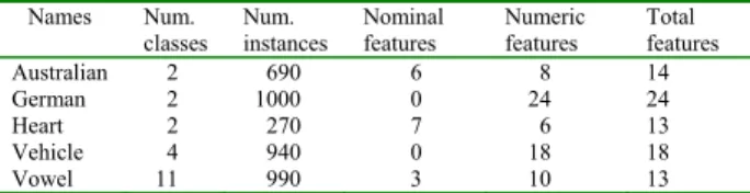
This section reports the experiments conducted to evaluate the classification accuracy of the proposed hybrid system using several real-world datasets from the UCI benchmark database [10]. These datasets consist of numeric and nominal attributes. Table 1 summarizes the number of numeric attributes, number of nominal attributes, number of classes, and number of instances for these datasets.
Table 1. Datasets used in the experiments.
Names Num.
classes Num. instances Nominal features Numeric features Total features Australian 2 690 6 8 14 German 2 1000 0 24 24 Heart 2 270 7 6 13 Vehicle 4 940 0 18 18 Vowel 11 990 3 10 13
Our implementation platform was carried out on the Matlab 7.3, by extending the Libsvm version 2.82 which is originally designed by Chang & Lin [11]. The empirical evaluation was performed on Intel Pentium IV CPU running at 3.4GHz and 1 GB RAM.
The GA-SVM approach was suggested by Huang [2] for searching the best C, γ and features subset, which deals solely with feature selection and parameters optimization by means of genetic algorithm. Experimental results from our proposed GA-DCNN-SVM hybrid method were compared with that from the GA-SVM algorithm. The detail parameter setting for genetic algorithm is as the following: population size 600, crossover rate 0.7, mutation rate 0.02, two point crossover, roulette wheel selection and the generation number 500. The best chromosome is obtained when the
termination criteria satisfy. We set nθm =20,
=20 and =20; the value of
c
n nr nf depends on the
experimental datasets described in Table 1. We
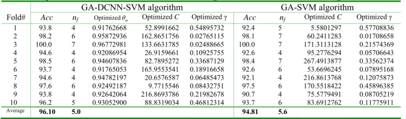
Table 2. Experimental results for Heart disease dataset using GA-DCNN-SVM and GA-SVM algorithms.
GA-DCNN-SVM algorithm GA-SVM algorithm
Fold# Acc nf Optimizedθm Optimized C Optimized γ Acc nf OptimizedC Optimized γ
1 93.8 4 0.91762668 52.8991662 0.54895732 92.4 5 5.5801297 0.57708836 2 98.2 6 0.95872936 162.8651756 0.02765115 98.1 7 60.2411283 0.01708658 3 100.0 7 0.96772981 133.6631785 0.02488665 100.0 7 171.3113128 0.21574369 4 94.6 4 0.92086954 26.9159661 0.10925755 92.6 4 95.2776294 0.05706643 5 98.5 6 0.94607836 82.7895272 0.33687129 98.4 7 267.4913877 0.33562374 6 93.7 4 0.91765053 165.9553541 0.18916658 92.6 6 53.6696245 0.07895168 7 94.6 4 0.94782197 20.6576587 0.06485473 92.1 4 216.8613768 0.12075873 8 97.6 6 0.92492187 9.7715546 0.08432751 97.5 6 170.5518422 0.45896385 9 93.8 4 0.92642064 216.8693786 0.21982678 90.7 4 75.5779491 0.08705219 10 96.2 5 0.93052900 88.8319034 0.46812314 93.7 6 83.6912762 0.11775911 Average 96.10 5.0 94.81 5.6
Table 3. Summary results on five UCI datasets
GA-DCNN-SVM GA-SVM
Name Avg_Acc Avg_n
f Avg_Acc Avg_nf Australian 90.25 4.3 88.17 4.5 German 87.38 12.6 85.64 13.1 Heart 96.10 5.0 94.81 5.6 Vehicle 85.92 8.6 84.06 9.7 Vowel 99.21 7.1 98.52 7.9
Taking the Heart disease dataset, for example,
the classification accuracy Acc, number of selected
features nf, and the best parametersθm, C, γ for
each fold using GA-DCNN-SVM algorithm and GA-SVM approach are shown in Table 2. For the GA-DCNN-SVM approach, average classification accuracy is 96.10%, and average number of features is 5.0. For GA-SVM algorithm, its average classification accuracy is 94.81%, and average number of features is 5.6. Table 3 shows the summary results for the average classification accuracy Avg_Acc and the average number of
selected features Avg_nf for the five UCI datasets
using the two approaches. Generally, compared with the GA-SVM algorithm, the proposed method has good accuracy performance with slightly fewer features and consistently outperforms the existing GA-based previously published approach.
5. Conclusion
In this paper, we first introduce a new DCNN data reduction algorithm to efficiently improve the
original CNN method.Second, we propose a novel
GA-DCNN-SVMhybrid model to simultaneously
optimize prototype construction, feature selection and parameters setting for SVM classifier. To the best of our knowledge, this is the first hybrid algorithm to integrate the data reduction, feature selection and parameters optimization for SVM. Compared with the GA-based previously published method, experimental results shows that our proposed hybrid model outperforms and exhibits the high efficiency for the SVM.
References
[1] V.N. Vapnik, The Nature of Statistical Learning
Theory, Springer-Verlag, NY, USA, 1995.
[2] C.L. Huang and C.J. Wang, “A GA-based feature selection and parameters optimization for support vector machines,” Expert systems with applications, vol. 31, pp. 231-240, 2006.
[3] P. Hart, “The condensed nearest neighbor rule,”
IEEE Trans. Info. Theory, vol. 14, pp. 515-516,
1968.
[4] W. Gates, “The Reduced Nearest Neighbor Rule,”
IEEE Trans. Information Theory, vol. 18, no. 3, pp.
431-433, 1972.
[5] F. Angiulli, “Fast Nearest Neighbor Condensation for Large Data Sets Classification,” IEEE Trans. Knowledge and data engineering, vol. 19, no. 11, pp. 1450-1464, 2007.
[6] F.S. Devi and M.N. Murty, “An Incremental Prototype Set Building Technique,” IEEE Trans. Information Theory, vol. 18, no. 3, pp. 431-433, 1972.
[7] M. Dash and H. Liu, “Feature selection for classification,” Pattern Recognition, vol. 35, no. 2, pp. 505-513, 2002.
[8] Z. Zhu, Y.S. Ong and M. Dash, “Wrapper-Filter Feature Selection Algorithm Using a Memetic Framework,” IEEE Trans. On Systems, MAN, and
Cybernetics, vol. 37, no. 1, pp. 70-76, 2007.
[9] C.W. Hsu, C.C. Chang, C.J. Lin, A practical guide to
support vector classification, Available at:
http://www.csie.ntu.edu.tw/~cjlin/papers/guide/gui de.pdf. 2003.
[10] S. Hettich, C.L. Blake, and C.J. Merz, UCI
repository of machine learning databases,
Department of Information and Computer Science, University of California, Irvine, CA., Available at: http://www.ics.uci.edu/~mlearn/MLRepository.htm, 1998.
[11] C.C. Chang, and C.J. Lin, LIBSVM: a library for
support vector machines, Software available at: