A new fuzzy clustering menthod with adjustable membership characteristics

全文

(1)A NEW FUZZY CLUSTERING METHOD WITH ADJUSTABLE MEMBERSHIP CHARACTERISTICS Dian-Rong Yang, Leu-Shing Lan, and Wei-Cheng Pao Department of Electronics Engineering National Yunlin University of Science and Technology, Taiwan ABSTRACT. development, we have analytically derived the formulae for cluster centers and the fuzzy partition matrix. Explicit formulae for the membership curves in a 1D two-cluster environment have also been derived to characterize the effects of the a1 and a2 parameters. Some examples are given to demonstrate the clustering results of this new scheme. The rest of this paper is organized as follows. In Section 2, we give a brief summary of the conventional fuzzy c-means algorithm. Then in Section 3, we present the new fuzzy clustering method with adjustable membership characteristics. The succeeding section presents analysis of membership functions. Some examples are given in Section 5. Finally Section 6 concludes this paper.. Clustering is an unsupervised procedure to group objects in accordance with their similarities. For nonseparable clusters, the concept of fuzziness is incorporated. Among other approaches, the fuzzy c-means algorithm is the most well-known fuzzy clustering method. In this work, we present a modified form of the fuzzy c-means based on a new definition of distance measure which can be considered as an extension of the conventional one. The key advantage of this new fuzzy clustering schemem is its ability to flexibly control the membership function curves. Analytical formulae have been derived for both cluster centers and the fuzzy partition matrix. Parameter effects related to the membership function curves have also been analyzed. Examples are given to demonstrate the clustering results of the newly presented scheme. Keywords: clustering, fuzzy clustering, fuzzy cmeans. 2. THE FUZZY C-MEANS ALGORITHM The fuzzy c-means algorithm [2] originated from an optimization problem. 1. INTRODUCTION. min U ,V. The process of subdividing a data set into distinct subsets with homogeneous elements is called clustering. For hard clustering, a membership value of zero or one is assigned to each pattern data. With fuzzy clustering, each datum belongs to all clusters simultaneously, but to different degrees. Cluster analysis has been extensively studied in various fields of engineering [1]. A variety of fuzzy clustering methods have been proposed, including fuzzy c-means [2], possibilistic c-means [3], noise clustering [4], fuzzy entropy clustering [5], credibilistic fuzzy c-means [6], convex-set-based fuzzy clustering [7], generalized weighted conditional fuzzy clustering [8], etc. This paper focuses on the extension of the well-known fuzzy c-means algorithm. Specifically, we propose a new distance measure which adds a higher-term to the original one. The net effect is that the membership curves can be controlled by adjusting two parameters a1 and a2 . Thus a more flexible clustering method is obtained. To facilitate the algorithm. subject to. 4. U,V ) = J(U. c X n X. xk − v i k2 (1) um ki kx. i=1 k=1 c X. uki = 1, ∀k. (2). i=1. where U is the fuzzy partition matrix, V is the collection of cluster centers, n is the number of data samples, c is the number of clusters, m is the weighting exponent, and uki is the membership value of x k with respect to cluster i. Optimality conditions at the stationary points require that Pn m k=1 ukix k P vi = (3) n m , ∀i k=1 uki −1  1 ¶ m−1 c µ 2 X x kx − v k k i  , ∀k, i (4) uki =  x k − v j k2 kx j=1 An alternating optimization procedure is commonly ulilized to solve the fuzzy c-means problem. The al1.

(2) From ∂∂L v i = 0, we have Pn m xk − v i k2 )x xk k=1 uki (a1 + 2a2 kx vi = P , ∀i n m 2 xk − v i k ) k=1 uki (a1 + 2a2 kx. ternating procedure consists of two steps: (1) fix cluster centers and find the fuzzy partition matrix, and (2) fix the fuzzy partition matrix and update cluster centers. Steps (1) and (2) are alternately executed until convergence is achieved. Note that the algorithm may converge to a local minimum or even a saddle point.. Substituting Eq. (9) into Eq. (7), one obtains Ã. 3. THE NEW FUZZY CLUSTERING METHOD WITH ADJUSTABLE MEMBERSHIP CHARACTERISTICS. αk = −. 4. min U ,V. U,V ) = J(U. c X n X. uki. subject to. uki = 1, ∀k. 2. Update the fuzzy partition matrix using Eq. (12). (6). 3. Update the cluster centers using Eq. (10).. (7). 4. Check for convergence. Usually this is done by U (k+1) − U (k) k ≤ ε. If not yet conchecking kU verged, go to Step 2 and proceed.. i=1. where U is the fuzzy partition matrix, V is the collection of cluster centers, n is the number of data samples, c is the number of clusters, m is the weighting exponent, and uki is the membership value of x k with respect to cluster i, for k = 1, · · · , n and i = 1, · · · , c. The necessary conditions for this optimization problem can be found using the method of Lagrange multipliers. First we define the corresponding Lagrangian function as L. 4. =. c X n X i=1 k=1 n X. αk. +. k=1. 4. ANALYSIS OF MEMBERSHIP FUNCTIONS In accordance with Eq. (12) one can define the membership function by  −1 1 ¶ m−1 c µ 2 4 X x x a kx − v k + a kx − v k 1 i 2 i  , ∀i x) =  fi (x x − v j k2 + a2 kx x − v j k4 a kx 1 j=1. xk − v i k2 + a2 kx xk − v i k4 ) um ki (a1 kx Ã c X. ! uki − 1.  −1 1 ¶ m−1 c µ 2 4 X xk − v i k + a2 kx xk − v i k a1 kx  , ∀k, i = xk − v j k2 + a2 kx xk − v j k4 a kx 1 j=1. 1. Initialize cluster centers. Usually this is performed by random assignment.. i=1 k=1 c X. 1. (12) The alternating algorithm of the conventional fuzzy cmeans method can also be applied to the new fuzzy clustering method with different updating functions for the cluster centers and fuzzy partition matrix. We summarize the solution algorithm as follows:. (5). xk − v i k2 um ki (a1 kx. xk − v i k4 ) +a2 kx. !−m+1. 1. xk − v i k2 + a2 kx xk − v i k4 )] m−1 [m(a1 kx (11) Eqs. (11) and (9) together yield. where x k is the kth input datum, v i is the ith cluster center, and a1 and a2 are two parameters specified by the user. With this new definition of distance measure, the fuzzy clustering problem can be reformulated as a new optimization problem 4. c X i=1. In convectional fuzzy c-means algorithm, the distance xk − v i k2 . We now extend this measure is defined by kx definition to include an additional higher-order term, namely, let us define the new distance measure by xk − v i k2 + a2 kx xk − v i k4 dki = a1 kx. (10). (13) where v i and v j are the centers for cluster i and j respectively. To gain more insight regarding how the parameters a1 and a2 affect the membership fuctions, let us focus on a specific situation with only two clusters where the feature vector possesses a single dimension and m = 2. Let the cluster centers of these two clusters be denoted by v 1 and v 2 respectively, and let x denote the Euclidean distance between the input datum and v 1 . Here we consider two different scenarios: (1) the input datum is located between v 1 and v 2 ; (2) v 1 is. (8). i=1. where αk is the corresponding Lagrange multiplier. At the optimal points of solutions, the partial derivatives of L with respect to all related variables should be equal ∂L = 0, we obtain to zero. From ∂u ki xk − v i k2 + a2 kx xk − v i k4 ) + αk = 0, ∀k, i mum−1 (a1 kx ki (9) 2. , ∀k.

(3) Inter−Center Distance (r) = 1. Inter−Center Distance (r) = 1. 1. 1. 0.9. 0.98. 0.8. 0.96. a2/a1 = 0 a /a = 1 2 1 a2/a1 = 10 a2/a1 = 100. 0.6. 0.94. Membership Value. Membership Value. 0.7. 0.5. 0.4. 0.92. 0.9. 0.88. 0.3. 0.86. 0.2. 0.84. 0.1. 0.82. 0. 0. 0.1. 0.2. 0.3. 0.4. 0.5. 0.6. 0.7. 0.8. 0.9. 0.8. 1. Euclidean Distance (x). a2/a1 = 0 a2/a1 = 1 a /a = 10 2 1 a2/a1 = 100. 0. 0.1. 0.2. 0.3. 0.4. 0.5. 0.6. 0.7. 0.8. 0.9. Fig. 1. The membership vs. Euclidean distance curve. Shown in this figure is the first scenario where the input datum is located between v 1 and v 2 .. Fig. 2. The membership vs. Euclidean distance curve. Shown in this figure is the second scenario where v 1 is located between the input datum and v 2 .. located between the input datum and v 2 . For the first scenario, we have. 5. EXAMPLES. ½ f1 (x) = =. 1+[. 1 a1 x2 + a2 x4 ] m−1 a1 (r − x)2 + a2 (r − x)4 (r − x)2 + aa21 (r − x)4. [x2 + (r − x)2 ] +. a2 4 a1 [x. + (r − x)4 ]. In this study we used an artificially synthesized data set for experimentation. This data set with 2000 data points comprises three non-overlapped clusters. Since the clusters are separable, the clustering task can be easily accomplished. However, with different fuzzy clustering strategies, varying fuzzy partition matrices can be generated. Figs. 3 through 6 show the experimental results. Prior to clustering, the data set went through a linear normalization operation so that each component of the feature vector is scaled to be in the range [0, 1]. In each figure, the scatter plot of input data are drawn with cluster centers and iso-membership contours overlaid. Each figure possesses a different combination of a1 and a2 values. From these figures, it is seen that cluster centers change slightly with varying combinations of a1 and a2 ; however, the iso-membership contours exhibit distinct changes. In principle, the larger the a2 /a1 ratio is, the higher the membership value is observed around the same neighborhood of a cluster center. Refer to Figs. 3 through 6 for the detailed contour plots.. ¾−1. (14). where r is the Euclidean distance between v 1 and v 2 . Similarly, for the second scenario we easily obtain ½ f1 (x) = =. 1+[. 1 a1 x2 + a2 x4 ] m−1 a1 (r + x)2 + a2 (r + x)4 (r + x)2 + aa21 (r + x)4. [x2 + (r + x)2 ] +. a2 4 a1 [x. + (r + x)4 ]. 1. Euclidean Distance (x). ¾−1. (15). From Eqs. (14) and (15) it is clearly seen that in both scenarios the memberships are affected by r and the ratio a2 /a1 . Figs. 1 and 2 show the membership vs. x curves. For the first scenario, with an increasing a2 /a1 ratio, the clustering gradually changes from soft partition toward harder partitions, as illustrated by Fig. 1. For the second scenario, we also observe that with an increasing a2 /a1 ratio, the clustering gradually changes from soft partition toward harder partitions, which is illustrated by Fig. 2. However, in the latter scenario, the changes occur at a slower pace.. 6. CONCLUSION Clustering plays a very important role in almost all branches of science and engineering. The conventional k-means and fuzzy c-means algorithms have been most popular methods for solving separable and non-separable clustering tasks. Based on a new definition of distance 3.

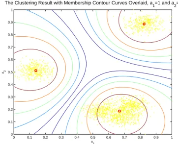
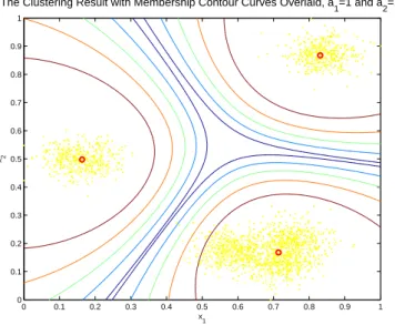
(4) measure, we propose a new form of fuzzy clustering method. The key distinct property of this new fuzzy clustering scheme is that it is capable of controlling the membership curve through adjusting the values of a1 and a2 . Further research will be necessary in order to characterize the choice of a1 and a2 values in a practical setting.. The Clustering Result with Membership Contour Curves Overlaid, a1=1 and a2=0 1. 0.9. 0.8. 0.7. 0.6 x2. 7. REFERENCES [1] A. Jain and R. Dubes, Algorithms for Clustering Data, Englewood Cliffs, NJ: Prentice-Hall, 1988.. 0.5. 0.4. 0.3. [2] J. bezdek, Pattern Recognition with Fuzzy Objective Function Algorithms, New York: Plenum, 1981.. 0.2. 0.1. 0. [3] R. Krishnapuram and J. Keller, “A Possibilistic Approach to Clustering,” IEEE Tr. Fuzzy Systems, Vol. 1, pp. 98-110, May 1993.. 0. 0.1. 0.2. 0.3. 0.4. 0.5 x1. 0.6. 0.7. 0.8. 0.9. 1. Fig. 3. An example to demonstrate the fuzzy clustering result. In this figure, a1 = 1 and a2 = 0, and cluster centers are shown as small red circles. For each cluster, five iso-membership contours are illustrated, which correspond to membership values of 0.9, 0.8, 0.7, 0.6 , and 0.5.. [4] R. N. Dave, “Characterization and Detection of Noise in Clustering,” Pattern Recognition Letters, Vol. 12, pp. 657-664, 1991. [5] D. Tran and M. Wagner, “Fuzzy Entropy Clustering,” Proc. IEEE 2000 Int’l Conf. Fuzzy Systems, pp. 152-157. [6] K. K. Chintalapudi and M. Kam, “A NoiseResistant Fuzzy c-Means Algorithm for Clustering,” Proc. IEEE 1998 Int’l Conf. on Fuzzy Systems, pp. 1458-1463.. The Clustering Result with Membership Contour Curves Overlaid, a1=1 and a2=1 1. 0.9. 0.8. [7] I. H. Suh, J.-H. Kim, and F. C.-H. Rhee, “ConvexSet-Based Fuzzy Clustering,” IEEE Tr. Fuzzy Systems, Vol. 7, No. 3, pp. 271-285, June 1999.. 0.7. 0.6 x2. [8] J. M. Leski, “Generalized Weighted Conditional Fuzzy Clustering,” IEEE Tr. Fuzzy Systems, Vol. 11, No. 6, pp. 709-715, Dec. 2003.. 0.5. 0.4. 0.3. 0.2. 0.1. 0. 0. 0.1. 0.2. 0.3. 0.4. 0.5 x1. 0.6. 0.7. 0.8. 0.9. 1. Fig. 4. An example to demonstrate the fuzzy clustering result. In this figure, a1 = 1 and a2 = 1, and cluster centers are shown as small red circles. For each cluster, five iso-membership contours are illustrated, which correspond to membership values of 0.9, 0.8, 0.7, 0.6 , and 0.5.. 4.

(5) The Clustering Result with Membership Contour Curves Overlaid, a1=1 and a2=10 1. 0.9. 0.8. 0.7. x2. 0.6. 0.5. 0.4. 0.3. 0.2. 0.1. 0. 0. 0.1. 0.2. 0.3. 0.4. 0.5 x1. 0.6. 0.7. 0.8. 0.9. 1. Fig. 5. An example to demonstrate the fuzzy clustering result. In this figure, a1 = 1 and a2 = 10, and cluster centers are shown as small red circles. For each cluster, five iso-membership contours are illustrated, which correspond to membership values of 0.9, 0.8, 0.7, 0.6 , and 0.5.. The Clustering Result with Membership Contour Curves Overlaid, a1=1 and a2=100 1. 0.9. 0.8. 0.7. x2. 0.6. 0.5. 0.4. 0.3. 0.2. 0.1. 0. 0. 0.1. 0.2. 0.3. 0.4. 0.5 x. 0.6. 0.7. 0.8. 0.9. 1. 1. Fig. 6. An example to demonstrate the fuzzy clustering result. In this figure, a1 = 1 and a2 = 100, and cluster centers are shown as small red circles. For each cluster, five iso-membership contours are illustrated, which correspond to membership values of 0.9, 0.8, 0.7, 0.6 , and 0.5.. 5.

(6)