AN ALGORITHM TO BUILD CONVEX HULLS FOR 3-D OBJECTS
Han-Ming Chen* and Tzung-Han Lin
ABSTRACT
In this paper, a new algorithm based on the Quickhull algorithm is proposed to find convex hulls for 3-D objects using neighbor trees. The neighbor tree is the data structure by which all visible facets to the selected furthest outer point can be found. The neighboring sequence of ridges on the outer boundary of all visible facets also can be found directly from the neighbor tree. This new algorithm is twice as efficient as Barber’s algorithm.
Key Words: 3-D convex hull, quickhull algorithm, computational geometry.
*Corresponding author. (Tel: 23680375; Fax: 886-2-23631755; Email: hmchen@ntu.edu.tw)
The authors are with the Department of Mechanical Engineering, National Taiwan University, Taipei, Taiwan 106, R.O.C.
I. INTRODUCTION
The convex hull of a set S of points is defined as the smallest convex set containing all the points in S. It is one of the most fundamental concepts in the field of computer graphics, computational geometry, pattern recognition, computer-aided design, image processing (Robert and Faugeras, 1995), and robotics. It also plays an important role in many applications such as shape determination (Kaasalainen and Torppa, 2001), collision detection (Sherali et al., 2001), find-ing the minimum boundfind-ing box (O’Rourke, 1993), a n d c o n s t r u c t i n g s p h e r i c a l V o r o n o i d i a g r a m (Sugihara, 2000).
Graham (1972) proposed an algorithm running in time complexity O(nlogn) for finding the convex hull of a set of planar points. Anderson reevaluated Graham’s algorithm for simplifying the computation to determine whether the second point in three con-secutive points is convex or not (Anderson, 1978). Later, several quick methods based on Graham’s al-gorithm were published to determine a 2-D convex hull for a set of planar points (Atwah et al., 1995; Atwah and Baker, 2002; Koplowitz and Jouppi, 1978). Jarvis presented a convex hull identification method that includes point deletion checks and is especially effective when the number of points on the plane is relatively small (Jarvis, 1973). In 1996, an algorithm that is a parallel adaptation of Jarvis March and the
Quickhull algorithm was presented by Atwah et al. (1996).
In recent decades, at least four algorithms for finding the multi-dimensional convex hull have been proposed. They are gift wrapping, divide and conquer, incremental, and Quickhull algorithms (O’Rourke, 1993). Chand and Kapur (1970) first presented the gift wrapping algorithm in arbitrary dimensions. In the gift wrapping algorithm, the convex hull of a point set is generated by continuing to find the hyperplane making the maximum interior angle with the adja-cent facet until all facets found are closed. Assume that the number of points is n. The gift wrapping algorithm runs in time O(n2). Sugihara revised the
conventional gift wrapping algorithm to increase nu-merical robustness and topological consistency and kept the same time complexity as the conventional algorithm (Sugihara, 1994).
The divide and conquer algorithm was first pro-posed by Preparata and Hong (1977) to apply a merge procedure for finding the convex hull of two non-in-tersecting convex hulls in two or three dimensions with O(nlogn) operations. A more detailed imple-mentation of the 3-D divide and conquer algorithm was presented by Day (1990).
O’Rouke (1993) presented a detailed implemen-tation for the incremental algorithm. Initially, one tetrahedral hull is formed by randomly selecting four non-degeneracy points. Each time a new tetrahedron is formed with an outside point and a triangle on the old hull. Afterward this new tetrahedron is merged into the old hull and the concave parts of the merged hull are filled up. The incremental algorithm is some-times called the beneath-beyond algorithm. Allison
and Noga (1997) combined the divide and conquer algorithm with the incremental algorithm in comput-ing 3-D convex hulls. In 3-D cases, the incremental algorithm requires O(nlogn) expected time (Clarkson and Shor, 1988; Edelsbrunner, 1987; Kallay, 1984; Mulmuley, 1994; Preparata and Shamos, 1985; Seidel, 1990). In each iterative routine of the incremental algorithm, the merged point is randomly selected so that the vertices of the convex hull can’t be found efficiently.
Generally speaking, the Quickhull algorithm is evolved from the incremental algorithm. In construct-ing 2-D convex hulls, Eddy (1977) presented a no-tion to successively partino-tion a set of planar points into several regions with binary trees. With the “throw-away” principle, Akl and Toussaint (1978) presented an algorithm in which the furthest outside point is selected for the selected edge of the current convex hull in each iterative routine and then the se-lected edge is replaced with two new edges. Instead of a triangle used by Eddy and a quadrilateral used by Akl (1978) and Bykat (1978) uses a line segment to divide planar points into two regions in the first step. For general-dimension Quickhull algorithms, Barber et al., (1996) proposed detailed procedures and empirical data. His algorithm is very efficient in con-structing general-dimension convex hulls.
In this paper, a new Quickhull algorithm for building 3-D convex hulls is presented. We propose some efficient routines to find a tetrahedron as the initial convex hull and then build successively the new convex hull for each new selected vertex. In finding the boundary of all visible facets for a new selected vertex, a neighbor tree is used in this paper. Because Barber’s algorithm is one of the latest and efficient Quickhull algorithms, the efficiency of our algorithm is compared with that of Barber’s algorithm.
II. METHODS
In some mathematical models, the vertex or facet enumeration is used for representing the convex hull. The vertex enumeration only contains all the vertices of the convex hull in random order. The facet enu-meration lists the inside halfspace for each facet of the convex hull. In this paper, each facet and its three neighboring facets of the current convex hull are recorded in a linked list. Compared with the data structures of previous Quickhull algorithms, a much simpler data structure is proposed in this paper to raise the efficiency of our algorithm. The procedure of our algorithm is described as follows and its pseudo-code is shown in Fig. 1 starting from the main routine CONVEX_HULL().
(1) Record all the points of input point set in a linked list Ls. Remove duplicated points from Ls with an
octree. Substitute the coordinate of each point in
Ls into four formulas x +y + z, x - y - z, -x + y - z,
and -x - y + z separately. Find out a point A in Ls
with the maximum value for the formula x + y + z and then take out point A from Ls. Repeat the same
process for points B, C, and D and remove them from Ls one by one. Points B, C, and D have the
maximum values for formulas x - y - z, -x + y - z, and -x - y + z respectively. Hence, points A, B, C, and D are definitely different. The initial tetrahe-dron is built with points A, B, C, and D if any three points of them are not collinear. The normal vec-tor of each facet of the initial tetrahedron must point outward. For each facet of the initial tetrahedron, its three neighboring facets are stored in a linked list. This part of the work has been done by the function FindInitialHull() in Fig. 1. (2) All the points in Ls are partitioned into five sets
by four facets of the initial tetrahedron in line (a) of Fig. 1. Four sets are outside the tetrahedron and the fifth set is inside the tetrahedron. For each facet Tn, if there are points in front of Tn, put Tn in
the tail of a linked list Lp. Otherwise, put Tn in
the tail of another linked list Le. After these four
facets have been put into Lp or Le, connect Le
af-ter Lp forming a new linked list Lh. Assume that
the head of Lh is the facet Tj.
(3) The work in line (b) of Fig. 1 is described as follows. If the facet Tj is NULL, the whole
pro-cedure has been finished and all facets in Lh form
the final convex hull. If Tj is inside the current
convex hull, remove Tj from the linked list Lh, set
the next facet in Lh as Tj, and then go back to step
(3). If there is no point in front of Tj, set the next
facet in Lh as Tj and then go back to step (3).
(4) Among all points in front of Tj, find the point P
furthest from Tj. In line (c) of Fig. 1, set the facet Tj as the root of a neighbor tree. Set three
neigh-boring facets of Tj as its three branches. Assume
that the node Tk is one of these three branches.
(5) For the node Tk, assume that the facet Ta is the
upper node of Tk and Ta, Tb, and Tc are three
neigh-boring facets of Tk in the neighbor tree. If Tk is
visible to point P, put Tb and Tc as two branches
of Tk into the neighbor tree in the same
surround-ing order as Ta, Tb, and Tc are around Tk on the
convex hull. If Tk has already appeared in this
neighbor tree, end the work of branch Tk. If Tk is
not visible to point P, set Tk as a boundary facet Bn and end the work of branch Tk. If there is any
branch Tk whose work has not been ended, go back
to step (5).
(6) Search the neighbor tree and take out the ridge shared by each boundary facet Bn and the upper
node facet of Bn with the depth-first search.
typedef struct {
FACET neighboringFacet*[3], *nextFacet; bool isInsideFacet = False;
int branchState[3]; /*record visible, repeated, or boundary for each neighboringFacet*/ VERTEX *frontVertex; /*the furthest point stored in the head of this linked list*/ } FACET;
NeighborTree(FACET *currentNode, VERTEX *furthest, VERTEX *outsideVertex, FACET *facetList) {
currentNode->isInsideFacet = True;
AddVertexToList(currentNode->frontVertex, outsideVertex); /*collect all points outside visible facets*/
for (each branch FACET Tk of currentNode) { if (Tk has not appeared in the tree) {
if (furthestVertex is in front of Tk)
SetbranchState(visible); /*Tk is a visible facet*/ else
SetbranchState(boundary); /*Tk is a boundary facet*/ }
else
SetbranchState(repeated); /*Tk is a repeated facet*/ }
for (each branch FACET Tj of currentNode) switch(branchState of Tj) {
case “visible”: /*Tj is a visible facet*/
NeighborTree(Tj, furthestVertex, outsideVertex, facetList); break;
case “boundary”: /*Tj is a boundary facet*/
newFacet = BuildOneFacet(); /*furthestVertex and two vertices shared by currentNode and Tj*/ RecordNewNeighbor(); /*replace currentNode with newFacet as one neighboring facet of Tj*/ AddToHead(newFacet, facetList);
break;
case “repeated”: /*Tj is a repeated facet*/ break;
default: break; }
}
PARTITION(VERTEX *vertexList, FACET *facetList, FACET *convexFacetList) {
for (each FACET Tn in facetList) { for (each VERTEX Pj left in vertexList)
if (VERTEX Pj in front of FACET Tn)
VertexAddToFacet(Pj, Tn); /*add Pj into the frontVertex of Tn*/ if (Tn->frontVertex != NULL) /*some points are in front of Tn*/
AddToList(Tn, convexFacetList);
/*in convexFacetList, add Tn after the last facet that has outside points*/ else /*no point is in front of Tn*/
AddToListTail(Tn, convexFacetList); /*add Tn into the tail of convexFacetList*/ }
}
CONVEX_HULL(VERTEX *vertexList) {
FACET *facetList, *convexFacetList = NULL; VERTEX *outsideVertex;
facetList = FindInitialHull(vertexList); /*build the initial tetrahedron*/ PARTITION(vertexList, facetList, convexFacetList); /*line (a)*/
for (each FACET Tj in convexFacetList) { /*line (b)*/ if (Tj->isInsideFacet) /*Tj is inside the convex hull*/
DeleteFacet(Tj); else {
if (Tj->frontVertex != NULL) {
Tj->FindBoundary(Tj, frontVertex, outsideVertex, facetList); /*line (c)*/
RecordNeighboringFacet(facetList); /*record neighboring facets for each new facet*/ Rearrange(facetList); /*avoid two successive facets neighboring on convex hull*/ PARTITION(outsideVertex, facetList, convexFacetList); /*line (d)*/
Tj = convexFacetList; /*go back to the head of convexFacetList after each partitioning*/ }
} } }
the new convex hull and put this facet into the tail of Lh. Collect all points outside the facets of the
new convex hull.
(7) In line (d) of Fig. 1, partition all outside points with each new facet formed in step (6) using the same process as step (2). Set j = j + 1 and go to step (3).
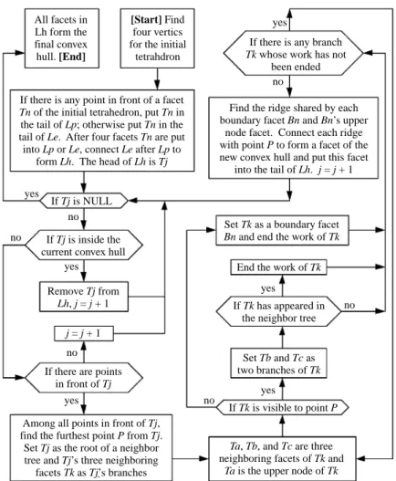
The procedures whole procedures of our algo-rithm whose starting point and terminal point are [Start] and [End] respectively is shown in Fig. 2.
For 3-D cases mentioned above, four vertices
A, B, C, and D are required to build the initial
tetrahedron. In 2-D cases, only three points P1, P3,
and P5 shown in Fig. 3 are needed to form the initial
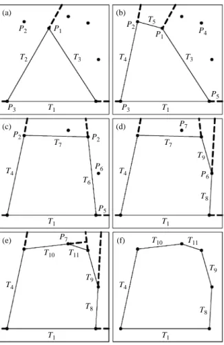
triangle. To demonstrate the whole procedure of our algorithm in a simpler way, a 2-D example is used. In order to describe one important process in our al-gorithm as shown in Fig. 3(b), the highest point in Fig. 3(a) is not chosen as one vertex, i.e., the point
P1, for the initial triangle.
In Fig. 3(a), all points are partitioned by facets in sequence of T1, T2, and T3. There are points in
front of T2 and T3 but there is no point in front of T1.
Facet T3 is after facet T2 in the partitioning sequence
so T3 is put after T2 in the linked list of Fig. 4(a) and
T1 is put in the tail of Fig. 4(a). Facet T2 is the first
element with outside points in Fig. 3(a) so T2 is set
as the root of the neighbor tree in Fig. 5(a). Among all points in front of T2 in Fig 3(a), find the furthest
point P2 from T2. Facets T1 and T3 are the
neighbor-ing facets of T2 and not visible to P2 so T1 and T3 are
the boundary facets of this tree and set as the branches of the root in Fig. 5(a). The ridge shared by T1 and
T2 is point P3 and the ridge shared by T2 and T3 is
point P1. Connect P2 to P3 and P1 separately to get
two new facets T4 and T5. All points which are in
front of T2 are partitioned by T4 and T5 to get Fig.
3(b) and Fig. 4(b). Facet T2 becomes an inside facet
in the current convex hull and is marked with a cross in Fig. 4(b) because T2 will not appear on the surface
of the final convex hull.
After T2 has been deleted in Fig. 3(b), T3
be-comes the first element with outside points in the linked list. Hence, set T3 as the root of the neighbor
tree and T1 and T5 as two branches of T3 in Fig. 5(b).
Among all points which are in front of T3, P4 is the All facets in
Lh form the final convex hull. [End]
If there is any point in front of a facet
Tn of the initial tetrahedron, put Tn in
the tail of Lp; otherwise put Tn in the tail of Le. After four facets Tn are put into Lp or Le, connect Le after Lp to
form Lh. The head of Lh is Tj
Find the ridge shared by each boundary facet Bn and Bn’s upper
node facet. Connect each ridge with point P to form a facet of the new convex hull and put this facet
into the tail of Lh. j = j + 1 [Start] Find
four vertics for the initial
tetrahdron
If there is any branch
Tk whose work has not
been ended yes no no If Tj is NULL If Tj is inside the current convex hull
Remove Tj from
Lh, j = j + 1
If there are points in front of Tj
j = j + 1
yes yes
no
Among all points in front of Tj, find the furthest point P from Tj.
Set Tj as the root of a neighbor tree and Tj’s three neighboring facets Tk as Tj’s branches
Ta, Tb, and Tc are three
neighboring facets of Tk and
Ta is the upper node of Tk
If Tk is visible to point P Set Tb and Tc as two branches of Tk If Tk has appeared in
the neighbor tree Set Tk as a boundary facet
Bn and end the work of Tk
End the work of Tk
no no yes yes yes no
furthest point from T3 in Fig. 3(b). Facet T1 is not
visible to P4 so T1 is set as a boundary facet in Fig 5
(b). Facet T5 is visible to P4 so T5 is set as a visible
facet. Aside from T3, T4 is another neighboring facet
of T5 and not visible to P4 so T4 is set as a boundary
facet. Facets T1 and T4 are two boundary facets to
P4. The ridge between T1 and its upper node, i.e., T3,
is P5. Point P2 is the ridge between T4 and its upper
node, i.e., T5. Connect P4 to P5 and P2 to form T6 and
T7 respectively. All points outside visible facets T3
and T5 are partitioned by T6 and T7. Facets T3 and T5
become inside facets in the current convex hull so they are marked with crosses in Fig 4(c). There are points outside T6 and T7 so T6 and T7 are inserted
suc-cessively into the linked list after T3 in Fig. 4(c).
Points P6 and P7 are the furthest points from T6
and T7 respectively in Fig. 3(c) and 3(d). After all
inside facets in Fig. 3(e) have been deleted, all the facets of the final convex hull are composed of T1,
T4, T8, T9, T10, and T11 as shown in Fig. 3(f) and 4(f).
Only the vertices of the initial triangle or the furthest points can be the vertices of the final convex hull in 2-D examples.
In Fig. 6(a) that is a 3-D example, light gray facets are visible and dark gray facets are not visible to the black point respectively. All visible facets and boundary facets are found with a neighbor tree. All ridges are located on the boundary between visible facets and invisible facets. Connect the black point to the two end points of each ridge to form a new facet. All visible facets will be inside the new con-vex hull so they will be deleted.
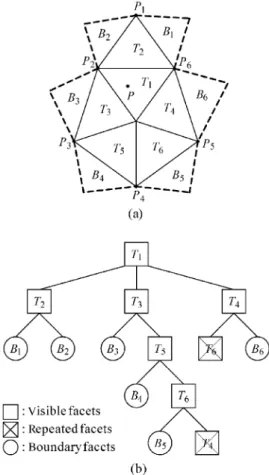
In the 3-D example shown in Fig. 7(a), assume (a) P2 T2 T3 P1 T1 P3 (b) P2 P5 T4 T5 T3 P4 P1 T1 P3 (c) P2 P6 P5 P2 T4 T6 T7 T1 (d) P6 T4 T7 T9 T8 P7 T1 (e) P7 T9 T4 T8 T10 T11 T1 (f) T4 T10 T11 T9 T8 T1
Fig. 3 A 2-D example and the processes of forming its final con-vex hull
Fig. 4 The linked lists for the 2-D example in Fig. 2
Fig. 5 Four neighbor trees for the 2-D example in Fig. 2
(a) (b)
Fig. 6 (a) Light gray facets are visible to the black point and dark gray facets are not visible to the black point. (b) Merge new facets into the old convex hull to form a new convex hull
that facet T1 is set as the root of the neighbor tree in
Fig. 7(b). Among all points that are in front of T1,
assume that P is the furthest point from T1. On the
convex hull, facets T1 through T6 are visible to P.
Facets T2, T3, and T4 are three neighboring facets of
T1 so set these three facets as the branches of T1.
Facets T1, B1, and B2 are three neighboring
fac-ets of T2 and their surrounding order around T2 in the
neighbor tree of Fig. 7(b) must be accorded with that around T2 on the convex hull of Fig. 7(a). Facet T1 is
the upper node of T2 so set B1, and B2 as two branches
of T2. Facets B1 and B2 are not visible to P so they
are boundary facets. Facets T1, B3, and T5 are three
neighboring facets of T3 and T1 is the upper node of
T3 so set B3 and T5 as two branches of T3. In the
similar way, B4 and T6 are set as two branches of T5
and B5 and T4 are set as two branches of T6. Facet T4
has already appeared in the neighbor tree so T4 is a
repeated facet. Facets B3, B4, and B5 are not visible
to P so they are boundary facets. Other parts of the neighbor tree are built in the same way. The bound-ary of all visible facets is found when every leaf node in a neighbor tree is either a boundary facet or a re-peated facet.
III. IMPLEMENTATION AND COMPARISON Assume that the plane equation of the facet A is
fA(x, y, z) = 0 and the coordinate of the point P is (xP, yP, zP). When building a neighbor tree in our algorithm,
if fA(xP, yP, zP) > –ε, facet A is defined as a visible
facet to point P. When doing the partitioning pro-cess in our algorithm, if fA(xP, yP, zP) > ε, P is
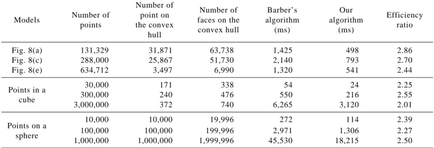
de-fined as a point in front of facet A. In this paper, the value of ε is set to 16 times of the machine epsilon (2.22E-16). Under these two conditions, degenerate cases will not cause any vague situation in our algorithm. Models in Figs. 8(a) and 8(c) were created by the software. The model in Fig. 8(e) was made with clay and then scanned with the laser scanning system to get image data. Figs. 8(b), 8(d), and 8(f) are the convex hulls of models Figs. 8(a), 8(c), and 8(e) respectively. The last six cases in Table 1 were cre-ated by random distribution of points in a unit cube or on the surface of a unit sphere respectively.
Our algorithm has been successfully implemented in C language with an Intel Pentium-4 1.6G personal computer. The source code of Barber’s algorithm is available via network address http://www.qhull.org/ download. In order to compare the net efficiency be-tween Barber’s algorithm and our algorithm, the time Fig. 7 (a) A 3-D example. (b) The neighbor tree of the example
in (a)
Fig. 8 Figures (a), (c), and (e) are three 3-D models. Figures (b), (d), and (f) are the convex hulls of models (a), (c), and (e) respectively
(a) (b)
(c) (d)
for reading data files is subtracted from the whole running time. Each datum in Table 1 is the average time for running the corresponding algorithm 30 times on the corresponding model.
For storing facets, double linked lists are used in Barber’s algorithm, but single linked lists are used in our algorithm. As a visible facet is deleted from the double linked list in Barber’s algorithm, the pre-vious element and the next element of the deleted facet will be connected. Hence, any element in the double linked list must have two pointers to the pre-vious element and the next element separately. In our algorithm, visible facets are found and marked in traversing the neighbor tree, and deleted in the next traverse of the linked list. Hence, the time for double linked lists is longer than that for linked lists in do-ing the similar work. This is the first point where our algorithm is better than Barber’s algorithm.
In Barber’s algorithm, the memory cell for each ridge is allocated first and then two neighboring facets and two endpoints are stored into this cell. Ridges found by Barber on the outer boundary of all visible facets are randomly stored and then these ridges form new facets with the furthest point. All new facets must be searched with a hash table to find neighboring rela-tions among them. This extra work is not necessary in our algorithm because the neighboring sequence of ridges appears in the neighbor tree. This is the second point where our algorithm is better than Barber’s algorithm. All outer points to visible facets must be parti-tioned by new facets which are formed with the outer boundary of these visible facets. In Barber’s algorithm, any two successively selected partitioning facets may be neighboring on the new convex hull. In our algorithm, two successively selected partitioning facets are arranged to avoid being neighboring facets on the new convex hull. Therefore, the total number of op-erations of substituting an outer point into the plane
equation of a partitioning facet in our algorithm is less than that in Barber’s algorithm. This is the third point where our algorithm is better than Barber’s algorithm.
The time complexity of our algorithm is O(nlogr), where n is the number of input points and r is the number of processed points. Although the time com-plexity order of our algorithm is the same as that of Barber’s algorithm, our algorithm is more efficient than Barber’s algorithm due to above three points in qualitative comparisons. In quantitative comparisons, the efficiency of our algorithm is over twice that of Barber’s algorithm for those nine models in Table 1.
IV. CONCLUSIONS
In this paper, the neighbor tree is proposed to find visible facets and ridges on the outer boundary of these visible facets. The data structure of our al-gorithm is simpler than that of Barber’s alal-gorithm. New facets found in our algorithm appear in neigh-boring sequence but these new facets must be arranged again in an extra process in Barber’s algorithm. The order of partitioning facets to partition outer points in our algorithm is more efficient than that in Barber’s algorithm. In both qualitative and quantitative comparisons, our algorithm is more efficient than Barber’s algorithm.
ACKNOWLEDGMENTS
We gratefully acknowledge the support of the National Science Council of the Republic of China for this research under the grant NSC 93-2212-E-002-061, and specially thank Ms. Yue-Jun Chen for mak-ing the clay model of Fig. 8(e) and Mr. Mmak-ing-Hui Lin for getting the image data of this model with the la-ser scanning system.
Table 1 The efficiency comparison between Barber’s algorithm and our algorithm on nine models Number of
Number of Barber’s Our
Number of point on Efficiency
Models faces on the algorithm algorithm
points the convex ratio
convex hull (ms) (ms) hull Fig. 8(a) 131,329 31,871 63,738 1,425 498 2.86 Fig. 8(c) 288,000 25,867 51,730 2,140 793 2.70 Fig. 8(e) 634,712 3,497 6,990 1,320 541 2.44 30,000 171 338 54 24 2.25 Points in a 300,000 240 476 550 216 2.55 cube 3,000,000 372 740 6,265 3,120 2.01 10,000 10,000 19,996 272 114 2.39 Points on a 100,000 100,000 199,996 2,971 1,306 2.27 sphere 1,000,000 1,000,000 1,999,996 45,530 18,215 2.50
REFERENCES
Akl, S. G., and Toussaint, G. T., 1978, “A Fast Con-vex Hull Algorithm,” Information Processing
Letters, Vol. 7, No. 5, pp. 219-222.
Allison, D. C. S., and Noga, M. T., 1997, “Comput-ing the Three-Dimensional Convex Hull,”
Com-puter Physics Communications, Vol. 103, No. 1,
pp. 74-82.
Anderson, K. R., 1978, “A Reevaluation of an Effi-cient Algorithm for Determining the Convex Hull of a Finite Planar Set,” Information Processing
Letters, Vol. 7, No. 1, pp. 53-55.
Atwah, M. M., Baker, J. W., and Akl, S. G., 1995, “An Associative Implementation of Graham’s Convex Hull Algorithm,” Proceedings of the
Sev-enth IASTED International Conference on Par-allel and Distributed Computing and Systems,
Washington D.C., USA, pp. 273-276.
Atwah, M. M., Baker, J. W., and Akl, S. G., 1996, “An Associative Implementation of Classical Convex Hull Algorithms,” Proceedings of Eighth
IASTED International Conference on Parallel and Distributed Computing and Systems, Chicago, IL,
USA, pp. 435-438.
Atwah, M. M., and Baker, J. W., 2002, “An Associa-tive Static and Dynamic Convex Hull Algorithm,”
Proceedings of the International Parallel and Dis-tributed Processing Symposium, Fort Lauderdale,
FL, USA, pp. 15-19.
Barber, C. B., Dobkin, D. P., and Huhdanpaa, H., 1996, “The Quickhull Algorithm for Convex Hulls,” ACM Transactions on Mathematical
Software, Vol. 22, No. 4, pp. 469-483.
Bykat, A., 1978, “Convex Hull of a Finite Set of Points in Two Dimensions,” Information
Process-ing Letters, Vol. 7, No. 6, pp. 296-298.
Chand, D. R., and Kapur, S. S., 1970, “An Algorithm for Convex Polytopes,” Journal of the Association for
Computing Machinery, Vol. 17, No. 1, pp. 78-86.
Clarkson, K. L., and Shor, P. W., 1988, “Algorithms for Diametral Pairs and Convex Hulls That Are Optimal, Randomized and Incremental,”
Proceed-ings of the Fourth Annual ACM Symposium on Computational Geometry, Urbana-Champaign,
IL, USA, pp. 12-17.
Day, A. M., 1990, “The Implementation of An Algorithm to Find The Convex Hull of a Set of Three-dimensional Points,” ACM Transactions on
Graphics, Vol. 9, No. 1, pp. 105-132.
Eddy, W. F., 1977, “A New Convex Hull Algorithm for Planar Sets,” ACM Transactions on
Math-ematical Software, Vol. 3, No. 4, pp. 398-403.
Edelsbrunner, H., 1987, Algorithms in Combinatorial
Geometry, Springer-Verlag, Heidelberg, Germany,
pp. 139-176.
Graham, R. L., 1972, “An Efficient Algorithm for Determining the Convex Hull of A Finite Planar Set,” Information Processing Letters, Vol. 1, No. 4, pp. 132-133.
Jarvis, R. A., 1973, “On the Identification of The Convex Hull of a Finite Set of Points in The Plane,”
Infor-mation Processing Letters, Vol. 2, No. 1, pp.
18-21.
Kaasalainen, M., and Torppa, J., 2001, “Optimization Methods for Asteroid Lightcurve Inversion,”
ICARUS International Journal of Solar System Studies, Vol. 153, No. 1, pp. 24-36.
Kallay, M., 1984, “The Complexity of Incremental Convex Hull Algorithms in Rd
,” Information
Pro-cessing Letters, Vol. 19, pp. 197.
Koplowitz, J., and Jouppi, D., 1978, “A More Effi-cient Convex Hull Algorithm,” Information
Processing Letters, Vol. 7, No. 1, pp. 56-57.
Mulmuley, K., 1994, Computational Geometry: An
Introduction Through Randomized Algorithms,
Prentice-Hall, Englewood Cliffs, NJ, USA, pp. 96-105.
O’Rourke, J., 1993, Computational Geometry in C, Cambridge University Press, New York, USA, pp. 113-167.
Preparata, F. P., and Hong, S. J., 1977, “Convex Hull of A Finite Set of Points in Two and Three Dimensions,” Communications of the ACM, Vol. 20, No. 2, pp. 87-93.
Preparata, F. P., and Shamos, M. I., 1985,
Computa-tional Geometry: An Introduction,
Springer-Verlay, New York, USA, pp. 95-145.
Robert, L., and Faugeras, O. D., 1995, “Relative 3D Positioning and 3D Convex Hull Computation from A Weakly Calibrated Stereo Pair,” Image and
Vision Computing, Vol. 13, No. 3, pp. 189-196.
Seidel, R., 1990, “Linear Programming and Convex Hulls Made Easy,” Proceedings of the Sixth
An-nual ACM Symposium on Computational Geometry,
Berkeley, CA, USA, pp. 211-215.
Sherali, H. D., Smith, J. C., and Selim, S. Z., 2001, “Convex Hull Representations of Models for Com-puting Collisions Between Multiple Bodies,”
European Journal of Operational Research, Vol.
135, No. 3, pp. 514-526.
Sugihara, K., 1994, “Robust Gift Wrapping for The Three-dimensional Convex Hull,” Journal of
Computer and System Sciences, Vol. 49, No. 2,
pp. 391-407.
Sugihara, K., 2000, “Three-Dimensional Convex Hull As a Fruitful Source of Diagrams,” Theoretical
Computer Science, Vol. 235, No. 2, pp. 325-337. Manuscript Received: Jul. 08, 2005 Revision Received: Dec. 15, 2005 and Accepted: Feb. 07, 2006