Location Classification of Nonstationary Sound
Sources Using Binaural Room Distribution Patterns
Jwu-Sheng Hu, Member, IEEE, and Wei-Han Liu
Abstract—This paper discusses the relationships between the
nonstationarity of sound sources and the distribution patterns of interaural phase differences (IPDs) and interaural level dif-ferences (ILDs) based on short-term frequency analysis. The amplitude variation of nonstationary sound sources is modeled by the exponent of polynomials from the concept of moving pole model. According to the model, the sufficient condition for utilizing the distribution patterns of IPDs and ILDs to localize a nonstationary sound source is suggested and the phenomena of multiple peaks in the distribution pattern can be explained. Simulation is performed to interpret the relation between the distribution patterns of IPD and ILD and the nonstationary sound source. Furthermore, a Gaussian-mixture binaural room distribution model (GMBRDM) is proposed to model distribution patterns of IPDs and ILDs for nonstationary sound source location classification. The effectiveness and performance of the proposed GMBRDM are demonstrated by experimental results.
Index Terms—Head-related transfer function (HRTF),
inter-aural level difference (ILD), interinter-aural phase difference (IPD), sound source localization.
I. INTRODUCTION
T
HE task of localizing a sound source using multiple mi-crophones has been developed for years [1]. Among var-ious kinds of techniques, methods that are based on the auditory system of humans or other animals using two microphones are one of the introduced approaches in this research field.The sound waves reaching a human listener are influenced by the listener’s body, as well as by the acoustic environment. The way that the human body modifies the incident sound waves is specified by head-related transfer function (HRTF), or by head-related impulse response (HRIR) [2]–[4]. The HRIR is a measure of impulse response from the sound source to eardrums in an anechoic room [5]. The HRTF is the Fourier transform of the HRIR [6]. The HRTF varies with the sound source location, and many localization cues based on the HRTF have been in-vestigated. For example, the interaural level differences (ILDs) and the interaural phase differences (IPDs) are major cues for localizing a sound source, especially for azimuth localization and these cues can be extracted from the HRTF [7].
Manuscript received April 16, 2008; revised October 24, 2008. Current ver-sion published April 15, 2009. This work was supported in part by the National Science Council of Taiwan under Grant NSC 95-2221-E-009-177, in part by the Ministry of Economics, Taiwan, under Grant 95-EC-17-A-04-S1-054, and in part by the Ministry of Education, Taiwan, under Grant 96W826. The as-sociate editor coordinating the review of this manuscript and approving it for publication was Dr. Jingdong Chen.
The authors are with Department of Electrical and Control Engi-neering, National Chiao-Tung University, Hsinchu 300, Taiwan (e-mail: jshu@cn.nctu.edu.tw; lukeliu.ece89g@nctu.edu.tw).
Digital Object Identifier 10.1109/TASL.2008.2011528
Brungart et al. concluded that ILDs play an important role in localizing sound sources near the head [8]. The IPD can be estimated by cross-correlation functions [9] or generalized cross-correlation methods [10], [11]. However, based on an as-sumption that head and ears are symmetrical, the sound source presented at a median plane should produce no interaural dif-ference. Therefore, interaural difference cues are insufficient for localizing the elevation of a sound source in the medium plane. Moreover, any sound source that falls on a “cone of confusion,” as Woodworth called it [12], may lead to constant IPDs and ILDs.
Cues of spectral modification are very important for elevation localization and front-back discrimination [13]–[17]. Generally, these elevation localization methods assume a flat sound source spectrum or one that is known in advance. However, these assumptions are not suitable for real appli-cations [13]. Another significant localization ability of the human auditory system is distance localization. Research works indicated that many possible cues exist for distance localization (e.g., overall sound source intensity and energy ratio of direct to reverberant sound [7], [18]). However, the former can only be employed for relative distance localization and the later is strongly influenced by the reflections in an indoor environment [7]. Therefore, sound source localization in three-dimensional environments using binaural information remains an open research topic.
Early experimental results for HRTF were principally ob-tained in anechoic rooms using the maximum-length sequence (MLS) method [19]. Hence, conventional studies of HRTF mainly concentrated on the steady-state response from a sound source to the eardrums caused by human body. Only a few studies addressed the issue of localizing a sound source in a reverberant room [14], [20]. However, for most sound source localization applications, the environments are reverberant and natural sounds are highly nonstationary [13]. These two factors could induce transient response and significantly influence the localization cues. Gustafsson et al. analyzed how reverberation can distort time-delay estimation [21]. Shinn-Cunningham et al. showed that HRTFs are altered by reverberant sound in a classroom [22], [23] and the reverberation can cause temporal fluctuation in short-term IPDs and ILDs [22]. These studies suggest that the performance of general methods of sound source localization based on a set of HRTFs measured in anechoic rooms with stationary sound sources could be limited because of the nonstationarity of natural sound, reverberation, and short-term frequency analysis. On the other hand, the work by Shinn-Cunningham [25] showed human listeners can adapt
to a reverberant environment, resulting in a better sound source localization performance than that in an anechoic room.
Recent work showed the benefit of temporal fluctuation phe-nomenon of IPDs and ILDs to sound source localization [26], [27]. Rather than eliminating the influence of the fluctuations, these studies attempted to describe the fluctuations using sta-tistical models and use them to classify the locations of sound sources. The work by Nix and Hohmann [26] investigated lo-calization cues of IPDs and ILDs exhibiting temporal fluctu-ation phenomena when sound sources are nonstfluctu-ationary and short-term frequency analysis, such as short-term Fourier trans-form (STFT), is utilized. In their work, distribution patterns of IPDs and ILDs were applied as location models to classify the azimuth and elevation of a sound source. Further, Smaragdis and Boufounos [27] also used the wrapped Gaussian model for the distribution pattern of relative magnitude and phase of the cross spectra in a reverberant room. Instead of estimating the azimuth, elevation or distance of sound source, the works of [26], [27] tried to build models for the distribution patterns and differen-tiated the location of sound source from modeled locations by using classification methods.
This study attempts to discuss how the amplitude variation of nonstationary sound sources could influence the distribution pattern of IPDs and ILDs when STFT is utilized. To simplify the description, distribution patterns of IPDs and ILDs are called binaural room distribution patterns (BRDPs) in remainder of this work. Although the nonstationarity of a sound source could be tested in many different domains [28], this work only considers the amplitude variation. The idea of moving pole model [29], [30] is employed to model the nonstationary sound sources; consequently, the amplitude variation is modeled as an exponent of polynomial. Based on this model, it can be shown that BRDPs depend on the content of the nonstationary source signals. The dependency is analyzed to explain the phenomenon of multiple peaks in the BRDPs.
Since the BRDPs can contain multiple peaks, a modeling method that deals with complicated distribution patterns is needed. This work adopts Gaussian mixture models (GMMs) [31] to model BRDPs (called Gaussian-mixture binaural room distribution model (GMBRDM)). Based on GMBRDM, this work can classify the sound source from one of the modeled locations using the pattern classification method. Because the GMBRDM is a linear combination of the phase difference GMM and the magnitude ratio GMM, a method is proposed to obtain the optimal weighting of the linear combination to enhance the classification ability. Additionally, because BRDPs contain information on direct paths and reflections, classify the location of a sound source in the azimuth, elevation and distance using the proposed GMBRDM is possible.
The remainder of this paper is organized as follows. The next section discusses how the nonstationary sound source could influence the IPD and ILD and a simulation of a simplified environment is performed to verify the discussion. Section III presents the formulation of the proposed GMBRDM. The experimental results are shown in Section IV and, finally, the conclusions are drawn in Section V.
II. RELATION BETWEEN THENONSTATIONARY
SOUNDSOURCE AND THEBRDP A. IPDs and ILDs of Nonstationary Sound Source
A linear time-invariant (LTI) room acoustic channel is repre-sented by a tapped finite impulse response (FIR) model
(1) where denotes sound signal emitted into the channel, denotes the signal received by the ear, and is the coefficients of the FIR model for the room impulse response (RIR) from sound source to an ear. Without loss of generality, the non-stationary input signal is assumed to be a complex exponen-tial signal with frequency and nonconstant amplitude . To model amplitude variation of a sound source, the amplitude of the complex exponential signal is assumed as time varying
(2) where represents the sampled frequency of an
-point STFT, is a integer between , and is a phase value between . For such an input, the corre-sponding output is
(3) Take the N-point STFT at frequency
(4) Since the analysis in this work assumes the signal is a com-plex exponential signal at one sampled frequency, the window function is omitted to simplify the expression. By denoting and as the signals received by left and right ears,
respectively, and and are the STFT of and
, the ratio between and is
(5) where and are the coefficients of FIR channel models, and , from the sound source to the left ear and the right
ear, , . The
FIR model of a room impulse response can be obtained through various approaches; for example, by real measurement in a room or by simulation. However, the derivation in this work is suitable for general FIR models, not specific ones.
Therefore, the IPD, , and ILD, , between
and are
and
(6)
where denotes the phase value. Note that the operation of nature logarithm is taken for computing the magnitude ratio. As shown in (6), the phase difference and magnitude ratio be-come content dependent when STFT is utilized and is non-stationary.
B. Modeling the Nonstationary Sound Source Using Moving Pole Model
To analyze how nonstationarity of a sound source influences the IPD and ILD, a parameterized model for nonstationary sound is needed. Based on the studies of modeling the nonsta-tionary sound source in [29] and [30], a nonstanonsta-tionary sound source in an analysis window can be expressed as a sum of moving pole models. In this work, the idea that approximate
as an exponent of polynomial is utilized [30]
(7) where is the degree of the polynomial, is the coefficient of the polynomial, and denotes the sampling frequency. To simplify the analysis, we omit the terms of , as proposed in [30]. Although omitting the higher order term would restrict the flexibility of the model; however, for the following STFT based analysis, this work assume that it is possible to find a suitable parameter of and to fit the amplitude variation. Hence, is modeled as
(8) Substituting (8) into (5) yields
(9) Through the same procedure, one can have
(10)
Fig. 1. Simulation configuration.
and the ratio between and becomes
(11) Consequently, the IPD and ILD are
and
(12)
By observing (12), this study finds that the IPD and ILD values depend on the coefficient of the FIR models and the value of . The FIR models correspond to the location of sound source and listener, and the value of corresponds to the slope of the nature logarithm of , which is the trend of amplitude variation of the sound source.
C. Content Dependency of BRDPs Obtained From Nonstationary Sound Source
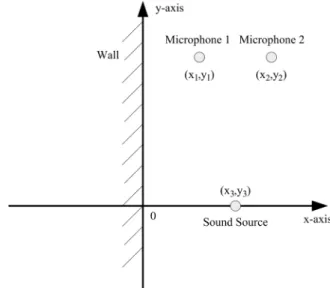
To verify the proposed analysis, a simplified simulation envi-ronment (Fig. 1) is assumed (Although the simplified environ-ment is utilized as an example here, the following discussion of the relationship between BRDPs and nonstationary sound sources can be applied to general cases).
As depicted in Fig. 1, the only cause of reflection is the infinite wall located at . The two microphones
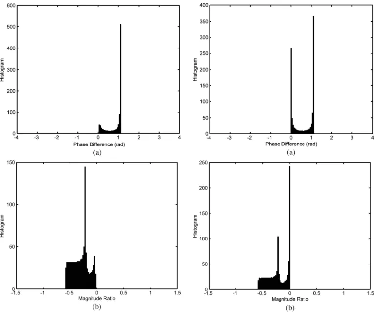
Fig. 2. Histograms of IPDs and ILDs of the first sound source. (a) The his-togram of IPDs of the first sound source. (b) The hishis-togram of ILDs of the first sound source.
m m m and the sound source
is located at m m m . The models
from the sound source to the microphones are simulated by the image method [32] with sound speed m/s and sampling rate Hz. The wall is assumed to be rigid, which means the reflection coefficient is 1. Therefore, the parameters of the FIR models are mostly determined by the geometrical relation among the sound source, microphones, and the wall. Two different sets of sound sources are input into the simulation model to show the content dependency of IPD and ILD histograms. For the first set of sound source, the value of is uniformly distributed between [ 500,0]. The IPDs and ILDs at a frequency of 140.625 Hz are computed 1000 times. Fig. 2 presents the histograms, which can represent the probability distribution, of IPDs and ILDs. The second set of sound source is similar to the first one, except the value of is uniformly distributed between [ 500,200]. Note that the value of is 0 for all simulation in this section; however, since
Fig. 3. Histograms of IPDs and ILDs of the second sound source. (a) The his-togram of IPDs of the second sound source. (b) The hishis-togram of ILDs of the second sound source.
is eliminated in the derivation of (12), changing this value would not influence the simulation results. The histograms are illustrated in Fig. 3.
The simulation results in Figs. 2 and 3 demonstrate that, when the sound sources are nonstationary, the IPD and ILD histograms depend on the content of the source signal. There-fore, conditions of the nonstationary sound source must be designed such that the BRDPs can be utilized for localization. In view of the discussion above, the sufficient condition is that the distribution of of the sound source must be stationary to make the sound source applicable for localization. Care must be exercised when using IPDs and ILDs obtained from nonstationary sound sources for sound source localization to avoid performance degradation.
D. Formation of Peaks in the Distribution Patterns of IPDs As shown by the simulation in Section III-A, the distribution patterns of IPDs exhibit multiple peaks. This phenomenon also
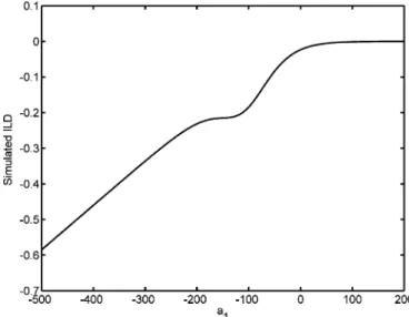
Fig. 4. Relation between the value ofa and the IPD.
appears in empirical results in real environments, as illustrated in the previous work [33]. The derivation result of (12) can be adopted to explain this phenomenon.
According to (12), there are several possible reasons to form peaks in the distribution patterns of IPDs. First, if of a sound source is concentrated at a certain value, a peak in the histogram will result. An example is a stationary sound source. For a sta-tionary sound source, for all measured frames, which makes IPD a fixed value, resulting in a peak in the distribution pattern.
Second, the term in (12) decreases as increases when is positive. This means the weighting of the reflection part in the channel model is reduced and the influence of the direct path is increased. Hence, when exceeds a certain level, the measured IPDs can be approximated as
(13)
where and are propagation delay of the direct path from the sound source to microphones. Based on (13), the phase difference caused by direct paths from a sound source to mi-crophones is emphasized and can dominate the measured IPDs. Since the IPDs are approximately the same for all exceed a certain level, a peak can be formed in the distribution pattern. This derivation explains why some previous research results of IPD-based time delay estimation suggested utilizing speech source onset to improve the accuracy [24]. On the the contrary, when is negative, the value of increases with . In this case, the influence of the direct path is suppressed and the reflections can dominate the measured IPDs.
The second simulation in Section II-C is utilized to interpret the relationship between and the IPD (Fig. 4).
In Fig. 4, as , the value of IPD approaches 0, which is the phase difference caused by the direct paths from the sound source to microphones. On the other hand, when , the value converges to 1.1, representing the phase difference in-fluenced by wall reflection. It is then easy to understand why
Fig. 5. Relation between the value ofa and the ILD.
there are two peaks at 0 and 1.1 in Fig. 3(a). Generally, reflec-tions appear later in the propagation model than direct paths, meaning that a negative value of is required to emphasize the effect of reflections. Consequently, the more the wall or boundary absorbs the energy of sound source, the more negative value of is required to emphasize the effect of reflections. E. Formation of Peaks in the Distribution Patterns of ILDs
There are two major reasons to result in peaks in the dis-tribution patterns of ILDs. First, if the of a sound source is concentrated at a certain value, it would result in a peak in the ILD distribution pattern. However, ILDs behave quite dif-ferently than IPDs when is either large or small. Based on the similar derivation of (13), when is larger than a certain level, can be approximated by
(14)
Therefore, the relationship between ILDs and is
approxi-mately linear (with a slope of ) when
is larger than a certain level. Hence, if the slope is 0 (meaning ), it will cause a peak in the ILD histogram. Similar to IPDs, when is smaller than a certain level, the influence of the direct path is de-emphasized and the reflection part starts dominating the measured ILDs. Fig. 5 shows the simulation re-sults for the relationship between the value of and the ILD.
In Fig. 5, when , the measured ILD is about 0
because the simulation sets and
. This results in a peak at 0 in the histogram, as shown in Fig. 3(b). In addition, when , the measured ILDs change linearly with the value of , resulting in a flat area in Fig. 3(b).
F. Location Classification of Nonstationary Sound Source Using BRDPs
As mentioned in the Introduction, classifying the location of sound sources presented at median plane or on a “cone of con-fusion” is difficult when only IPDs and ILDs of direct paths
are utilized. However, sound sources at different locations can propagate through different reflections and with the property of nonstationary sound source discussed above, the nonstationary sound can result in distinguishable distribution patterns. Con-sequently, it is possible to classify the location of the sound sources in the azimuth, elevation, and distance using BRDPs.
III. GMBRDM FOR NONSTATIONARY
SOUNDSOURCELOCALIZATION
As discussed in Section II-C, if the environment and head position are unchanged and the distribution of of the sound source is stationary, using BRDPs to classify the locations sound sources is possible. Sections II-D and II-E also show that BRDPs can be non-Gaussian and contain multiple peaks. Consequently, modeling these distribution patterns as a simple distribution pattern (such as a single Gaussian distribution) can eliminate important details. However, utilizing a high-resolu-tion normalized histogram to model the distribuhigh-resolu-tion pattern requires considerable memories. In this paper, GMMs are employed to model BRDPs (called the GMBRDM) to reduce the memory requirement through parameterization.
A. Training Procedure of the Proposed GMBRDM
Let and denote the phase difference
and magnitude ratio obtained at frame , respectively, for
con-structing GMM at frequency , , which means
frequencies are utilized to construct the model. The phase dif-ference and magnitude ratio GMMs are defined as the weighted sum of and mixtures of Gaussian component densities
(15)
(16)
where ,
. and are the
weighting of ith mixture, and and are
the Gaussian density function. Notably, the mixture weights must satisfy the constraints
and (17)
The terms and represent the parameters of and component densities
and (18)
where
denotes the phase difference mixture weight vector with
dimensions ;
denotes the magnitude ratio mixture weight vector with
dimensions ;
denotes the phase difference mean matrix with dimensions
;
denotes the magnitude ratio mean matrix with dimensions ; denotes the phase difference covariance matrix with
dimensions ;
denotes the magnitude ratio covariance matrix with
dimensions .
The parameters and in (18) can be estimated by the EM algorithm [31], [34] which guarantees a monotonic increase in the model’s log-likelihood value. By denoting the training sequence length as , the iterative procedure can be divided into the expectation step and maximum step
1) Expectation step:
(19)
(20)
where and are
poste-riori probabilities. 2) Maximization step:
a) Estimate the mixture weights:
(21)
(22)
b) Estimate the mean vector:
(23)
c) Estimate the variances:
(25)
(26)
The EM algorithm is sensitive to the choice of initial model. A good choice of initial model results in a lower number of it-erations of the EM algorithm. K-means based methods are fre-quently used for determining the initial model parameters. This work utilizes an accelerated K-means algorithm proposed by Elkan [35] to find the initial value of and . The initial
values of and are set to and
, respectively. The variances of Gaussian all components are initialized as 1.
The proposed GMBRDM at each location is defined as the linear combination of the phase difference GMM and the mag-nitude ratio GMM
(27) where , and represent the weighting factors. The values of and can be chosen arbitrarily. However, poor choices of these parameters would lead to a poor clas-sification result. This work provides a method to determine these parameters based on the sum of the correlation values among locations of the phase difference GMM and magnitude ratio GMM. It uses the sum of correlation of IPDs’ GMMs, , and the sum of correlation of
ILDs’ GMMs, , among
dif-ferent locations. If the IPDs’ GMMs among difdif-ferent locations have higher correlation, it means they are more similar to each other and the chance to discriminate them is considered lower (so does the ILDs’ GMMs among different locations). Conse-quently, the GMMs with higher correlation should lead to lower weight, since the ability to discriminate is considered lower under this circumstance, and vice versa. Under this principle,
and are determined by the following formula:
(28)
where and are the dimensional random
vectors in the operation ranges, and
and .. . . .. .. . ... . .. .. . ... ... ... with dimension In addition (29) (30) and (31)
where and denote the total selected numbers of
and .
The values of and can be obtained by solving (28) as
(32)
(33) The proofs of (32) and (33) are shown in the Appendix. B. Testing Procedure of the Proposed GMBRDM
The location of a sound source is classified by finding the maximum a posteriori probability from GMBRDMs for a given
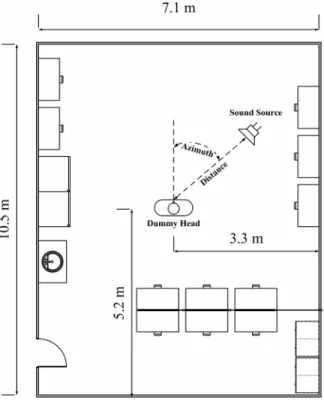
Fig. 6. Layout of the experimental environment.
observation sequence. Since the GMBRDMs are location de-pendent, finding the most possible GMBRDM of a given test sequence also gives the most possible location classification
(34)
where and
are the phase difference and mag-nitude ratio computed from the testing sequences denoted as and , and denotes the testing sequence length.
The probabilities and could be selected
as since the probability in each location is equally likely for a blind search. Moreover, because the probability densities and are the assumed same and conditionally independent for all location models, the localization rule can be recast as
(35)
IV. EXPERIMENTALRESULTS
The experiment is performed in a laboratory filled with common furniture and equipment. Fig. 6 shows the layout of the environment.
Fig. 7. Dummy head adopted in the experiment.
The laboratory area is m and room height is 3 m. The recording equipment comprises two B&K 4935 array microphones, a B&K 2694 conditioning amplifier, and an Azova DAQP-16 analog-to-digital converter. The microphones are mounted in the ears of a dummy head, as depicted in Fig. 7. The distance between the dummy head’s ears is 0.16 m. Fig. 6 illustrates the location of the dummy head. The ears of the dummy head are placed 1 m above the floor.
The sound source is a recording of a female reading a book in Mandarin (Here, we assume the distribution of of the speech signal remains identical during training and testing procedure.). The sound source is generated by a loudspeaker. Received sig-nals are sampled at 8000 Hz, and the STFT window is 512 sam-ples. For each experiment, the sound source is played at each lo-cation to obtain the training sequence to establish GMBRDMs. Training sequence length is set to 400 and testing sequence length is set to 100, with a shift of 80 samples between each frame. Hence, 4-s data are utilized for training, and 1-s data are utilized for testing; note that the training sequence and the testing sequence are nonoverlapping word sets. Since this work attempts to classify the sound source location, the testing sequences are always generated from one of the trained loca-tions. Six significant frequencies of the sound source, which are 250, 484.4, 578.1, 734.4, 796.9, and 1140.6 Hz, are selected in all experiment. Note that the number “six” is obtained form em-pirical results. Generally, add more significant frequencies im-prove the localization performance at the expense of more com-putational load. These frequencies are obtained by observing the major peaks of average spectrum of sound source. There-fore, each Gaussian model has six dimensions . For each location, testing is performed 100 times to acquire the correct rate. In this experiment, if the location of a sound source is clas-sified to the nearest trained location in the database, it will be regarded as a correct one.
The first experiment tests the ability of azimuth classification. In this experiment, distances between the sound source and ears
TABLE I
AVERAGECORRECTRATES OFAZIMUTHCLASSIFICATION ATEACHDISTANCE
TABLE II
AZIMUTHCLASSIFICATION AT THEDISTANCE OF 2.0 m
AND THENUMBER OFMIXTURES IS25
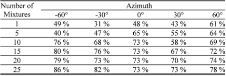
are fixed at 1, 1.2, 1.4, 1.6, 1.8, and 2 m. For each distance, the azimuth of sound source moves from 60 , 30 , 0 , 30 , to 60 to test the average correct rate of azimuth classification. The elevation of sound source is set the same as that of the ears (1 m). Different numbers of mixtures are utilized. Table I shows the average correct rate of azimuth classification at each distance.
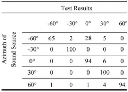
As shown in Table I, when the distance between the sound source and ears is 1 m, meaning that the sound source close to the dummy head, the performance of only one mixture is roughly the same as those of high numbers of mixtures. When the sound source is close to the dummy head, the influence of direct path propagation is much more significant than that of re-verberations. Consequently, the BRDPs are influenced less by the reflections and can be modeled using a single Gaussian dis-tribution model. However, as distance between the sound source and ears increases, the influence of reflection is becoming sig-nificant and leads to complex BRDPs. The benefit of adopting multiple mixtures is apparent at a long distance, such as 2 m, where the correct rate increases with the number of mixture. Table II shows the detail of classification at the distance of 2.0 m and the number of mixtures is 25. One hundred trials were taken for sound source at each angle, and the entry in Table II repre-sents the number estimated for each angle. It is shown that at azimuth of 60 , a great deal of misclassification occurs at 0 while for the case of 0 , none of the trials is misclassified to
60 . The testing sequence is much shorter than the training se-quence. This result indicates that at shorter sequence, the model at 60 could be similar to the one at 0 but not vice versa.
The histogram of IPDs measured with frequency 250 Hz at 60 and 0 are illustrated in Fig. 8 as an example to explain the cause of this result. As shown in Fig. 8, besides the peak at the phase difference around 1.2 rad, the histogram of IPDs
Fig. 8. Histograms of IPDs measured with frequency of 250 Hz. (a) At azimuth of060 . (b) At azimuth of 0 .
obtained at 60 also contains peaks at the phase difference around 0 rad, which is overlapped with those in the histogram of IPDs obtained at 0 . When the testing sequence is much shorter than the training sequence, the measured IPDs may only con-centrates around 0 rad and result in classification error.
The second experiment tests the capability of the proposed GMBRDM for distance classification. In this experiment, the azimuth is fixed at 60 , 30 , 0 , 30 , and 60 . At each az-imuth, the distance between the sound source and ears changes from 1, 1.2, 1.4, 1.6, 1.8, to 2 m to acquire average correct rates. The sound source height is adjusted to 1 m. Table III shows the average correct rates for distance classification at each azimuth. Because the relationship between the sound source and ears meets the criterion of far-field, the IPDs of direct path at the same azimuth and different distances are approximately iden-tical theoreiden-tically. The ILDs of direct paths generate only rela-tively a slight difference between distant locations. Thus, mod-eling these BRDPs using a single Gaussian component can lose
TABLE III
AVERAGECORRECTRATES OFDISTANCECLASSIFICATION ATEACHAZIMUTH
TABLE IV
AVERAGECORRECTRATES OFELEVATIONCLASSIFICATION ATEACHAZIMUTH
important details caused by reflections and result in poor local-ization results. As listed in Table III, the average correct rates when only one mixture is employed are clearly lower than those with a high number of mixtures. This experimental finding is be-cause the proposed GMBRDM can represent the details of the BRDPs for superior modeling results.
The third experiment tests the elevation classification perfor-mance of the proposed GMBRDM. In this experiment, distance between the sound source and ears is 2 m and the azimuth is fixed at 60 , 30 , 0 , 30 , and 60 . At each azimuth, the el-evation of the sound source changes from 1 m, 1.25 m, to 1.5 m (or 0 , 7 , to 14 , approximately) to acquire average cor-rect rates. Table IV lists experimental results. Experimental data show that GMBRDM with a large number of mixtures can prop-erly model the BRDPs at different elevations.
V. CONCLUSION
This paper investigates the relationship between nonsta-tionary sound sources and the BRDPs when STFT is utilized. Firstly, the amplitude variation of the nonstationary sound source is modeled as an exponent of polynomial based on the concept of moving pole model. This model explains the content dependency of the BRDPs. Moreover, the sufficient condition for utilizing BRDPs to classify the location of nonstationary sound source is identified. The phenomena of multiple peaks in the distribution patterns are analyzed. The related derivation shows that using simple distribution, such as a single Gaussian distribution, is not suitable for modeling these distribution patterns. Therefore, a GMBRDM is proposed to model the BRDPs for classifying the locations of nonstationary sound sources. Experimental results display that the proposed GM-BRDM can discriminate between the azimuth, elevation, and distance of the sound sources. Notably, the correct rates in experimental results do not monotonically increase with the number of Gaussian mixtures. This experimental finding is because the proposed GMBRDM can be influenced by the
initial condition selected and the complexity of BRDPs varies with sound source locations. However, the initial condition of the GMM remains an open research topic in the field of pattern recognition and statistics. A more appropriate method to obtain the initial values of GMBRDM could improve the performance of proposed method further. Moreover, the proposed method is unsuitable for unknown or changing environments since the relationship between BRDPs and the sound source locations can only be obtained using empirical data. Prediction of this relationship requires further research.
APPENDIX
Proofs of (32) and (33). The problem is formulated as
(A1) According to the constraint, set . Then, the cost function becomes
(A2)
Setting the first derivative with respect to be zero gives
(A3) Therefore
(A4)
(A5)
REFERENCES
[1] M. Brandstein and H. Silverman, “A practical methodology for speech source localiration with microphone arrays,” Comput., Speech, Lang., vol. 11, no. 2, pp. 91–126, Apr. 1997.
[2] F. L. Wightman and D. J. Kistler, “Headphone simulation of free-field listening. I: Stimulus synthesis,” J. Acoust. Soc. Amer., vol. 85, pp. 858–867, Feb. 1989.
[3] F. L. Wightman and D. J. Kistler, “Headphone simulation of free-field listening. II: Psychophysical validation,” J. Acoust. Soc. Amer., vol. 85, pp. 868–878, Feb. 1989.
[4] S. Carlile, Virtual Auditory Space: Generation and Application. New York: Chapman & Hall, 1996.
[5] W. G. Gardner and K. D. Martin, “HRTF measurements of a KEMAR,”
J. Acoust. Soc. Amer., vol. 97, no. 6, pp. 3907–3909, Jun. 1995.
[6] H. S. Colburn and A. Kulkarni, “Models of sound localization,” in
Sound Source Localization, Springer Handbook of Auditory Research,
R. Fay and T. Popper, Eds. New York: Springer-Verlag, 2005. [7] J. C. Middlebrooks and D. M. Green, “Sound localization by human
listeners,” Annu. Rev. Psychol., vol. 42, pp. 135–159, Jan. 1991. [8] D. S. Brungart, N. I. Durlach, and W. M. Rabinowitz, “Auditory
lo-calization of nearby sources. II Lolo-calization of a broadband source,” J.
Acoust. Soc. Amer., vol. 106, no. 4, pp. 1956–1968, Oct. 1999.
[9] C. Trahiotis, L. R. Bernstein, R. M. Stern, and T. N. Buell, “Interaural correlation as the basis of a working model of binaural processing: An introduction,” in Sound Source Localization, Springer Handbook of
Au-ditory Research, R. Fay and T. Popper, Eds. New York: Springer-Verlag, 2005.
[10] C. H. Knapp and G. C. Carter, “The generalized correlation method for estimation of time delay,” IEEE Trans. Acoust., Speech, Signal
Process., vol. ASSP-24, no. 4, pp. 320–327, Aug. 1976.
[11] G. C. Carter, A. H. Nuttall, and P. G. Cable, “The smoothed coher-ence transform,” IEEE Signal Process. Lett., vol. SPL-61, no. 10, pp. 1497–1498, Oct. 1973.
[12] R. S. Woodworth, Experimental Psychology. New York: Halt, 1938. [13] P. M. Hofman and A. J. von Opstal, “Spectro-temporal factors in two-dimensional human sound localization,” J. Acoust. Soc. Amer., vol. 103, no. 5, pp. 2634–2648, May 1998.
[14] J. P. Blauert, Spatial Hearing. Cambridge, MA: MIT Press, 1983. [15] V. R. Algazi, C. Avendano, and R. O. Duda, “Elevation localization and
head-related transfer function analysis at low frequencies,” J. Acoust.
Soc. Amer., vol. 109, no. 3, pp. 1110–1122, Mar. 2001.
[16] P. Zakarouskas and M. S. Cynader, “A computational theory of spectral cue localization,” J. Acoust. Soc. Amer., vol. 94, no. 3, pp. 1323–1331, Sep. 1993.
[17] J. C. Middlebrooks, “Narrow-band sound localization related to external ear acoustics,” J. Acoust. Soc. Amer., vol. 92, no. 5, pp. 2607–2624, Nov. 1992.
[18] B. G. Shinn-Cunningham, “Distance cues for virtual auditory space,” in Proc. IEEE Int. Conf. Multimedia, Dec. 2000, pp. 227–230. [19] D. D. Rife and J. Vanderkooy, “Transfer-function measurement using
maximum-length sequences,” J. Acoust. Soc. Amer., vol. 37, no. 6, pp. 419–444, Jun. 1989.
[20] W. M. Hartmann, “Localization of sound in rooms,” J. Acoust. Soc.
Amer., vol. 74, no. 5, pp. 1380–1391, Nov. 1983.
[21] T. Gustafsson, B. D. Rao, and M. Trivedi, “Source localization in rever-berant environments: Modeling and statistical analysis,” IEEE Trans.
Speech Audio Process., vol. 11, no. 6, pp. 791–803, Nov. 2003.
[22] B. G. Shinn-Cunningham, N. Kopcp, and T. J. Martin, “Localizing nearby sound sources in a classroom: Binaural room impulse re-sponse,” J. Acoust. Soc. Amer., vol. 117, no. 5, pp. 3100–3115, May 2005.
[23] B. G. Shinn-Cunningham, “Localizing sound in rooms,” in Proc. ACM
SIGGRAPH EUROGRAPHICS Campfire: Rendering Virtual Environ.,
May 2001, pp. 17–22.
[24] J. Huang, N. Ohnishi, and N. Sugie, “Sound localization in reverberant environment based on the model of the precedence effect,” IEEE Trans.
Instrum. Meas., vol. 46, no. 4, pp. 842–846, Aug. 1997.
[25] B. Shinn-Cunningham, “Learning reverberation: Considerations for spatial auditory displays,” in Proc. Int. Conf. Auditory Display, Apr. 2000, pp. 126–133.
[26] J. Nix and V. Hohmann, “Sound source localization in real sound fields based on empirical statistics of interaural parameters,” J. Acoust. Soc.
Amer., vol. 119, no. 1, pp. 463–479, Jan. 2006.
[27] P. Smaragdis and P. Boufounos, “Position and trajectory learning for microphone arrays,” IEEE Trans. Audio, Speech, Lang. Process., vol. 15, no. 1, pp. 358–368, Jan. 2007.
[28] Y. H. Tsao, “Tests for nonstationarity,” J. Acoust. Soc. Amer., vol. 75, no. 2, pp. 486–498, Feb. 1984.
[29] D. H. Friedman, “Estimation of formant parameters by sum-of-poles modeling,” in Proc. ICASSP, Apr. 1981, pp. 351–354.
[30] F. Casacuberta and E. Vidal, “A nonstationary model for the anal-ysis of transient speech signals,” IEEE Trans. Acoust., Speech, Signal
Process., vol. ASSP-35, no. 2, pp. 226–228, Feb. 1987.
[31] D. A. Reynolds and R. C. Rose, “Robust text-independent speaker iden-tification using Gaussian mixture speaker models,” IEEE Trans. Speech
Audio Process., vol. 3, no. 1, pp. 72–83, Jan. 1995.
[32] J. B. Allen and D. A. Berkley, “Image method for efficiently simu-lating small-room acoustics,” J. Acoust. Soc. Amer., vol. 65, no. 4, pp. 943–950, Apr. 1979.
[33] J. S. Hu, W. H. Liu, C. C. Cheng, and C. H. Yang, “Location and orien-tation detection of mobile robots using sound field features under com-plex environments,” in Proc. IEEE/RSJ Int. Conf. Intellig. Rob. Syst., Oct. 2006, pp. 1151–1156.
[34] G. Xuan, W. Zhang, and P. Chai, “EM algorithms of Gaussian mixture model and hidden Markov model,” in IEEE Int. Conf. Image Process., Oct. 2001, pp. 145–148.
[35] C. Elkan, “Using the triangle inequality to accelerate k-means,” in Proc.
20th Int. Conf. Mach. Learn., 2003, pp. 147–153.
Jwu-Sheng Hu (M’94) received the B.S. degree from
the Department of Mechanical Engineering, National Taiwan University, Taiwan, in 1984, and the M.S. and Ph.D. degrees from the Department of Mechanical Engineering, University of California at Berkeley, in 1988 and 1990, respectively.
From 1991 to 1993, he was an Assistant Professor in the Department of Mechanical Engineering, Wayne State University, Detroit, MI. In 1993, he joined the Department of Electrical and Control Engineering, National Chiao-Tung University, Hsinchu, Taiwan, and became a Full Professor in 1998. He served as the Vice-Chairman of the Department since 2006, and since 2008, he has worked in-part at the Industrial Technology Research Institute (ITRI) of Taiwan, where he serves as an Advisor for the Intelligent Robotics Program. His current research interests include robotics, microphone array, active noise control, and embedded systems.
Dr. Hu received the Research Initiation Award from the National Science Foundation while at Wayne State University.
Wei-Han Liu was born in Kaohsiung, Taiwan, in
1977. He received the B.S., M.S., and Ph.D. degrees in electrical and control engineering from National Chiao-Tung University, Hsinchu, Taiwan, in 2000, 2002, and 2007, respectively.
Dr. Liu is the winner of the TI DSP Solutions Design Challenge in 2000 and of the national competition held by Ministry of Education Advisor Office in 2001. He is the winner of the Best Paper Award at IEEE/ASME 2002. His research interests include sound source localization, microphone array signal processing, adaptive signal processing, speech signal processing, and robot localization.