利用超音波感測及電腦視覺技術經由簡易學習作自動車導航之研究

全文

(1)國立交通大學多媒體工程研究所碩士論文. 利用超音波感測及電腦視覺技術經由簡易學習作自動車導航之研究 A Study on Mobile Robot Navigation with Simple Learning Procedures by Ultrasonic Sensing and Computer Vision Techniques. 研究生：蔡雙圓指導教授：蔡文祥. 中華民國. 教授. 九十七. 年六月.

(2) 利用超音波感測及電腦視覺技術經由簡易學習作自動車導航之研究 A Study on Mobile Robot Navigation with Simple Learning Procedures by Ultrasonic Sensing and Computer Vision Techniques. 研究生：蔡雙圓. Student：Shung-Yung Tsai. 指導教授：蔡文祥. Advisor：Wen-Hsiang Tsai. 國立交通大學多媒體工程研究所碩士論文. A Thesis Submitted to Institute of Multimedia Engineering College of Computer Science National Chiao Tung University in partial Fulfillment of the Requirements for the Degree of Master in. Computer Science June 2008 Hsinchu, Taiwan, Republic of China. 中華民國九十七年六月.

(3) 利用超音波感測及電腦視覺技術經由簡易學習作自動車導航之研究. 研究生：蔡雙圓. 指導教授：蔡文祥博士. 國立交通大學多媒體工程研究所. 摘要本研究提出了兩套智慧型自動車系統，其一是以視覺為基礎的自動巡邏車，具有利用跟隨人物同時做學習路徑、與人互動、二維影像分析以及路徑規劃等功能；其二為利用超音波訊號分析做智慧型導航的自動車。我們利用一台具有 PTZ 攝影機的自動車作為實驗平台，並且利用有線網路與自動車通訊，使其航行於室內環境中。針對一利用格狀圖案為校正目標的舊有影像校正方法，我們提出了一精確的十字中心自動偵測方法，增進了校正的準確性與自動化。我們也建立了一計步器校正技術，用一校正模型來減少自動車所累積的行走機械誤差。接著我們發展一利用動態調整跟隨人物衣服顏色參考值的方法，來適應跟隨人物時環境中的不均勻照度。針對跟隨人物在自動車前的快速消失，我們亦提出一利用攝影機轉動角度，紀錄使用者方向的尋找方法，並使用一增加參考圖素數量的方法，來增進偵測人物朝向的準確率。當使用者要求自動車進行學習時，自動車能夠從影像中自動找出需要被監控的物品。此外，我們利用最小化均方差以及動態選擇門檻值，來規劃跟隨人物時所學習的路徑。我們同時提出一分析串列超音波訊號的方法，使自動車能在狹窄的室內空間中進行導航。最後我們以成功的巡邏、跟隨和導覽實驗證明本系統的完整性與可行性。. i.

(4) A Study on Mobile Robot Navigation with Simple Learning Procedures by Ultrasonic Sensing and Computer Vision Techniques. Student: Shung-Yung Tsai. Advisor: Prof. Wen-Hsiang Tsai, Ph. D.. Institute of Multimedia Engineering, College of Computer Science National Chiao Tung University. ABSTRACT Two intelligent autonomous vehicle systems for use in indoor environment applications are proposed. One is a vision-based vehicle system for security patrolling which has the capabilities of learning paths by person following, interaction with humans, analyzing 2D images and conducting path planning. Another is an intelligent vehicle system for navigation by analyzing ultrasonic signals. A vehicle equipped with wired control and a web PTZ camera is used as a test bed. First, a method for improving the practicability of an adopted camera calibration method is proposed, which uses a grid pattern as the calibration target and detects the centers of cross shapes on the pattern in a more precise and automatic manner. Next, a technique of odometer calibration is proposed, which uses an odometer calibration model to reduce the incremental mechanical errors the vehicle suffers. Besides, a technique for person following in an environment with variant illuminations is proposed, which adjusts the reference color value for person following dynamically. To follow a target person who turns fast in front of the vehicle, a technique of using the image information exhibited by the angle of panning of the camera to search the disappearing person is proposed. Also proposed is a technique for enhancing the accuracy of detection of the facing direction of a human by increasing the number of pixels for use in the detection work. ii.

(5) For object monitoring, the vehicle is enabled to find out the 2D object in the image automatically when the followed person asks it to learn the object. In addition, a minimum MSE technique for refining dynamically the path learned while following a person is proposed. Finally, a method of vehicle navigation in corridor environments by the use of the ultrasonic signal sequence is proposed. Good experimental results show the flexibility and feasibility of the proposed methods for the applications of security patrolling, person following, and people guiding in indoor environments.. iii.

(6) ACKNOWLEDGEMENTS I am in hearty appreciation of the continuous guidance, discussions, support, and encouragement received from my advisor, Dr. Wen-Hsiang Tsai, not only in the development of this thesis, but also in every aspect of my personal growth. Thanks are due to Mr. Chih-Jen Wu, Mr. Kuan-Chieh Chen, Mr. Jiun-Tsung Wang, Mr. Guan-Lin Huang, Miss Hsing-Chia Chen, and Mr. Li-Jyun Lyu for their valuable discussions, suggestions, and encouragement. Appreciation is also given to the colleagues of the Computer Vision Laboratory in the Institute of Computer Science and Engineering at National Chiao Tung University for their suggestions and help during my thesis study. Finally, I also extend my profound thanks to my family for their lasting love, care, and encouragement. I dedicate this dissertation to my beloved parents.. iv.

(7) CONTENTS ABSTRACT (in Chinese) .............................................................................................i ABSTRACT (in English).............................................................................................ii ACKNOWLEDGEMENTS .......................................................................................iv CONTENTS..................................................................................................................v LIST OF FIGURES ...................................................................................................vii Chapter 1 1.1 1.2 1.3 1.4 1.5 Chapter 2. Introduction.............................................................................................1 Motivation..................................................................................................1 Survey of Related Studies ..........................................................................3 Overview of Proposed Approach ...............................................................4 Contributions..............................................................................................6 Thesis Organization ...................................................................................8 System Configuration and Guidance Principles................................10. 2.1 2.2. Introduction..............................................................................................10 System Configuration .............................................................................. 11 2.2.1 Hardware configuration ...............................................................12 2.2.2 Software configuration.................................................................13 2.3 Learning Strategy and Major Steps in Proposed Process ........................14 2.4 Path Planning and Patrolling Principle and Major Steps in Proposed Process ....................................................................................................15 2.5 Vehicle Navigation Principle and Major Steps in Proposed Process .......17 Chapter 3. Camera and Odometer Calibration ....................................................21. 3.1 3.2. Introduction..............................................................................................21 Camera Calibration by Cross Shape Detection........................................22 3.2.1 Idea of Proposed Camera Calibration Method.............................22 3.2.2 Coordinate Systems and Directional Angles of Camera..............23 3.2.3 Review of Adopted Camera Calibration Method.........................25 3.2.4 Proposed Cross Shape Detection Technique................................29 3.3 Odometer Calibration by Quadratic Functions ........................................34 3.3.1 Idea of Odometer Calibration ......................................................34 3.3.2 Odometer Calibration Model .......................................................34 3.3.3 Curve Fitting ................................................................................37 3.3.4 Navigation by Odometer Calibration...........................................41 v.

(8) Chapter 4. Learning Procedures ............................................................................43. 4.1 4.2. Introduction..............................................................................................43 Human Following ....................................................................................43 4.2.1 Review of Adopted Method .........................................................43 4.2.2 Proposed Improvement of Adopted Process ................................45 4.2.3 Person Tracking Strategy .............................................................48 4.3 Learning of Path Data ..............................................................................51 4.4 Detection of Human Facing Direction.....................................................52 4.4.1 Review of Adopted Process .........................................................52 4.4.2 Proposed Improvement of Adopted Process ................................54 4.5 Learning of 2D Objects............................................................................57 4.5.1 Review of adopted algorithm for learning of objects ..................57 4.5.2 Learning 2D Objects Automatically ............................................60 4.5.3 Finding Regions of 2D Objects....................................................61 4.5.4 Finding the Horizontal Line Automatically .................................64 Chapter 5. Path Planning by Minimizing Mean Square Errors Using Ultrasonic Signals ....................................................................................................69. 5.1 5.2 5.3 5.4 Chapter 6. Introduction..............................................................................................69 Path Planning by MSE criterion ..............................................................70 Dynamic Path Decomposition .................................................................73 Vehicle Navigation by 2D Object Image Matching.................................75 ALV Navigation by Ultrasonic Signal Sequences ..............................80. 6.1 6.2. Ultrasonic sensing in ALV System ..........................................................80 Principle of Navigation ............................................................................81 6.2.1 Learning Strategy.........................................................................81 6.2.2 Navigation Strategy .....................................................................82 6.3 Applications in Tour Navigation..............................................................86 6.4 Experimental Results ...............................................................................86 Chapter 7 7.1 7.2 Chapter 8 8.1 8.2. Experimental Results and Discussions ...............................................91 Experimental Results ...............................................................................91 Discussions ..............................................................................................98 Conclusions and Suggestions for Future Works ..............................100 Conclusions............................................................................................100 Suggestions for Future Works................................................................102. References .................................................................................................................104 vi.

(9) LIST OF FIGURES Figure 1.1 Flowcharts of proposed systems...................................................................8 Figure 2.1 Equipment connection situations in this study. ..........................................12 Figure 2.2 The vehicle Pioneer 3 used in this study. (a) A front view of the vehicle. (b) A side view of the vehicle........................................................................13 Figure 2.3 The pan-tilt-zoom camera used in this study. (a) A perspective view of the camera. (b) A front view of the camera. (c) A left-side view of the camera. ..................................................................................................................14 Figure 2.4 An illustration of the automatic learning process by person following......16 Figure 2.5 An illustration of the path planning process. ..............................................18 Figure 2.6 An illustration of the patrolling process. ....................................................19 Figure 2.7 An illustration of the learning process of the vehicle navigation system. ..19 Figure 2.8 An illustration of the navigation process. ...................................................20 Figure 3.1 The coordinate systems used in this study. (a) The image coordinate system. (b) The global coordinate system (c) The vehicle coordinate system. (d) The spherical coordinate system..............................................................24 Figure 3.1 The coordinate systems used in this study. (a) The image coordinate system. (b) The global coordinate system (c) The vehicle coordinate system. (d) The spherical coordinate system. (continued) .........................................25 Figure 3.2 The pan angle of the camera. (a) 0 ≤ θ c ≤ π . (b) 0 ≥ θ c ≥ −π . ................26 Figure 3.3 The tilt angle of the camera. (a) 0 ≤ ϕc ≤. π 2. . (b) 0 ≥ ϕc ≥ −. π 2. . ...............27. Figure 3.4 An illustration of transformation between image coordinate system (ICS) and spherical coordinate system (SCS)....................................................28 Figure 3.5 Camera calibration by a vertical grid board. (a) An illustration of attaching the lines on the wall. (b) The intersections seen by camera are marked by yellow points............................................................................................28 Figure 3.6 The camera views of Figure 3.5. (a) View of Figure 3.5(a). (b) View of Figure 3.5(b). ...........................................................................................29 Figure 3.7 Detection of the cross point of a cross shape. (a) The look of a cross shape. (b) A center point and four lines composing the cross shape. (c) A circle with four intersections with the cross shape. (d) Use of four lines to detect the cross shape. ........................................................................................31 Figure 3.8 The matrix used to detect the cross shape. .................................................31 Figure 3.9 Some experimental results of cross shape detection. (a) Original Image. (b) After thresholding. (c) Find groups of centers. (d) Center detected. (e) The bmp image with camera calibration information..............................32 vii.

(10) Figure 3.9 Some experimental results of cross shape detection. (a) Original Image. (b) After thresholding. (c) Groups of centers detected. (d) Centers detected. (e) The bmp image with camera calibration information. (continued) ....33 Figure 3.10 The program window of camera calibration. ...........................................33 Figure 3.11 An illustration of the experiment. .............................................................36 Figure 3.12 The distribution of the angles of the deviations. ......................................36 Figure 3.13 The results of line fitting of the angle of deviation. .................................40 Figure 3.14 An illustration of odometer calibration.....................................................42 Figure 4.1 An illustration of proposed learning procedures. .......................................44 Figure 4.2 The application for person following. ........................................................46 Figure 4.3 The top-view of light and illumination in the hallway. ..............................47 Figure 4.4 An illustration of improvement of adopted process. ..................................48 Figure 4.5 An illustration of person tracking strategy..................................................49 Figure 4.6 An example of person tracking results. (a) A vehicle is following a person. (b) The person turns fast to right. (c) The vehicle turns an angle θfind to find the person. (d) The vehicle finds the person. (e) The vehicle follows the person again. ......................................................................................50 Figure 4.7 Drafts of maps. (a) Map of an open indoor environment. (b) Map of a hallway environment................................................................................51 Figure 4.8 An illustration of detection of a person’s facing direction. ........................53 Figure 4.9 An illustration of the facing direction of the person. (a) Front. (b) Back. (c) Left. (d) Right. .........................................................................................53 Figure 4.10 An illustration of the scan rectangle for human facing direction detection. (a) Front. (b) Back. (c) Left. (d) Right.....................................................56 Figure 4.11 (a) A red rectangle including the monitored object as an interesting region. (b) A user interface to specify the horizontal line. ...................................58 Figure 4.12 The relative position C(xr, yr) of the vehicle with respect to the start point in the world coordinate system. ...............................................................58 Figure 4.13 An illustration of learning of a monitored object automatically...............62 Figure 4.14 Sobel Operator (a) x direction (b) y direction. .........................................64 Figure 4.15 The relationship with x-y space and γ-θ space. ........................................65 Figure 4.16 The accumulation array A of the Hough Transform. ................................66 Figure 4.17 An example of detection of information of monitored object by the progressive method. (a) An image with a monitored object. (b) The thresholding result. (c) The interesting region. (d) The horizontal line...67 Figure 4.17 An example of detection of information of monitored object by the progressive method. (a) An image with a monitored object. (b) The thresholding result. (c) The interesting region. (d) The horizontal line. viii.

(11) (continued) ...............................................................................................67 Figure 4.18 Another example of detection of information of monitored object by the progressive method. (a) An image with a monitored object. (b) The thresholding result. (c) The interesting region. (d) The horizontal line...67 Figure 4.18 Another example of detection of information of monitored object by the progressive method. (a) An image with a monitored object. (b) The thresholding result. (c) The interesting region. (d) The horizontal line. (continued) ...............................................................................................68 Figure 5.1 Illustrations of path planning. (a) Backing to the start point directly. (b) Stepping on every path node precisely. (c) The planned path we desire. 70 Figure 5.2 Illustration of proposed path planning........................................................72 Figure 5.3 An illustration of proposed dynamic path decomposition..........................74 Figure 5.4 Computation of the turning angle and move distance. ...............................76 Figure 5.5 An example of a planned path of an ellipse shape......................................77 Figure 5.6 An illustration of proposed patrolling process. ..........................................78 Figure 5.7 An example of experimental results. (a) The vehicle monitors an object. (b) The vehicle walks to a turning point (c) The vehicle monitors another object. (d) The vehicle goes back to the original start point. ...................79 Figure 6.1 The positions of ultrasonic sensors around the vehicle. .............................81 Figure 6.2 An illustration of the parameter of Width. (a) The hallway with two walls. (b) The hallway only has one wall...........................................................82 Figure 6.3 An illustration of the parameter of Directiondetect (a) Directiondetect = left. (b) Directiondetect = right. (c) Directiondetect = left + right. (d) Directiondetect = front.............................................................................83 Figure 6.4 An illustration of the situation of adjusting the direction of the vehicle. (a) The vehicle should turn an angle to the right (b) The vehicle should turn an angle to the left....................................................................................85 Figure 6.5 An illustration of navigation in a hallway...................................................85 Figure 6.6 The navigation path. (a) An example of paths. (b) The path is transformed into an automation....................................................................................87 Figure 6.7 An experimental result of navigation in an indoor environment. (a) The vehicle navigates on the path. (b) The navigation map............................88 Figure 6.7 An experimental result of navigation in an indoor environment. (a) The vehicle navigates on the path. (b) The navigation map. (continued) .......89 Figure 6.7 An experimental result of navigation in an indoor environment. (a) The vehicle navigates on the path. (b) The navigation map. (continued) .......90 Figure 7.1 An interface of the experiment. The green box shows the image stream and the blue box shows the input image at this moment. The yellow box ix.

(12) shows the difference image and the red box shows the draft of the map.92 Figure 7.2 An experimental result of extraction of the clothes. (a) The input image. (b) The image of the extracted clothes. .........................................................93 Figure 7.3 An experimental result of the learning mode. (a) The input image. (b) The position of the vehicle..............................................................................93 Figure 7.4 An example result of learning a 2D object. (a) The input image. (b) The region of the 2D object. (c) The horizontal line of the 2D object............94 Figure 7.5 An experimental result of following a person turning fast. (a) The input image. (b) The position of the vehicle. ....................................................94 Figure 7.5 An experimental result of following a person turning fast. (a) The input image. (b) The position of the vehicle. (continued).................................95 Figure 7.6 An experimental result of navigation. The blue line segments show the planning result. And the red points show the real patrolling path of the vehicle. .....................................................................................................95 Figure 7.7 The experimental result of object monitoring and navigation path correction. (a) The numbers of monitored objects. (b) The vehicle monitors the objects. (c) The matching result and the horizontal line used for path correction....................................................................................96 Figure 7.8 An illustration of the path of following a person and monitoring objects in an experiment...........................................................................................96 Figure 7.9 Interfaces of the experiment. ......................................................................97 Figure 7.10 An illustration of learned data and navigation path..................................97 Figure 7.11 An experimental result of navigation........................................................97 Figure 7.12 The experimental result of the vehicle guide a person. (a) Navigation in a hallway. (b) Navigation at a turning point. ..............................................98. x.

(13) Chapter 1 Introduction. 1.1 Motivation In recent years, autonomous land vehicles with ultrasonic sensors and vision-based robots have played helpful roles in human life. They can help us to do various tasks, such as: (1) keeping company with old people like a nurse to take care of them; (2) monitoring concerned objects; (3) navigating in desired environments automatically; (4) guiding people in indoor environment, and so on. In security monitoring of objects, if we use stationary cameras, we have to install many of them and there might still be corners where the cameras cannot cover. But if we use an autonomous vehicle equipped with a video camera, which has the ability of automatic learning and human following, then the problem can be solved because the vehicle can follow people everywhere and learns the path that we hope it patrol, just like a mother teaching her child where to go. While a vehicle follows a person, the vehicle has to detect the person in front of it continually. However, this is not easy because the brightness could not be all the same on the path, it could change to dark or bright slowly, and the person in the camera view might be darker or brighter than in the view a moment ago. The vehicle has to keep finding out the person to follow under variant brightness. When the vehicle is patrolling, it may seem not smart if it walks totally the same 1.

(14) as the trajectory it learned, because this trajectory could be rough and there is no need to step on every spot of it precisely. We hope the vehicle could reconstruct the path into a smooth route, but not too smooth to miss some important points we want it to patrol. In playing the role of a guide, it might be dangerous when the vehicle guides people in a narrow environment because the vehicle could hit the wall. But if we use an autonomous land vehicle equipped with ultrasonic sensors, the problem can be solved because the vehicle can then detect the distance to the wall using ultrasonic signals and keep navigating in the middle of the path safely. For the application of person guidance, the vehicle needs often the additional functions of making audio introductions to the environment or the surrounding objects, and making warning announcements to people who stand on the way that the vehicle want to pass through. In summary, the research goal of this study is to design an intelligent autonomous vehicle system with two kinds of capability. One is to learn the traversed path and objects which to be monitored, while following a person, and then navigate to the start point by automatic path correction by the use of computer vision and ultrasonic sensing techniques. For this goal, it is desired to design a system to be capable of automatic learning and path planning. The other capability is to navigate in a narrow indoor environment by ultrasonic sensing. It is desired to design a system to be capable of environment analysis in narrow indoor environments. By these functions, a variety of applications of the vehicle can be carried out, like being used as an autonomous patrolling assistant or a security guard, as well as a guide in an office environment, an exhibition area, or a tour route.. 2.

(15) 1.2 Survey of Related Studies To achieve the mission of person following in indoor environments, the function of human detection is required at first for finding a targeted person in the person following process. Skin color is an important feature of humans. In the study of human skin colors, many methods have been proposed to build skin color models. Wang and Tsai [1] proposed a method which uses an elliptic skin model to detect human faces by color and shape features in images. They also proposed another method which detects a person not using the skin color, but using the colors of the clothes which the person wears. A study of human detection under variant illumination was conducted by Chen and Tsai [2]. They used many sets of color values of Cb and Cr to define a function of skin-color reference models. The function was then used to separate human skin regions from background. Besides, some systems for person following have been proposed. Ku and Tsai [3] proposed a sequential pattern recognition method to decide the location of a person with respect to a vehicle and to detect a rectangular shape attached on the back of the person to achieve smooth person following. However, the person has to appear in the image all the time and the road has to be wide enough for this method to work. In applications of person following, Kwolek [4] proposed a method that determines the position of a mobile robot by laser readings. The tracking of the human head is done by a particle filtering technique using the features of color, depth, gradient, and shape. Morioka, Lee, Hashimoto [5] studied person following to provide people with services by the use of a human collaborative robot which tracks the back and shoulder of a person. There are some different studies for human detection and following by using different sensors. Treptow, Cielniak, and Duckett [6] proposed a method which tracks and identifies people from thermal and gray images. 3.

(16) For object monitoring, the vehicle has to learn the features of the concerned object and match the features to determine whether the object is the same as the previously learned one. Lowe [7] used a scale-invariant detector to find the extrema in the difference-of-Gaussian scale-space. He then created a scale-invariant feature transform (SIFT) descriptor to match key points using a Euclidean distance metric in. an efficient best-bin first algorithm which can identify the nearest neighbors of points in high dimensional spaces. For path planning, a method for planning the navigation task for a mobile robot under dynamic and unknown environments was proposed by Xiao, Liao, and Zhou [8]. For the topic of robot navigation, Chen and Tsai [9] proposed a method with a simplified SIFT for monitoring objects and used the position and feature information of objects to conduct vehicle navigation. Davison [10] proposed a method for monocular vision-based robot navigation.. 1.3 Overview of Proposed Approach The goal of this study, as mentioned previously, is to design two kinds of intelligent capabilities for autonomous land vehicles. One is to use computer vision and ultrasonic sensing techniques for person following and patrolling. The other is to use ultrasonic sensing for navigation in narrow indoor environments. The overall frameworks of proposed systems for these two capabilities are illustrated in Figure 1.1(a) and Figure 1.1(b). The first proposed approach to person following and patrolling using a vision-based autonomous vehicle with an ultrasonic sensing system includes seven major stages. The first stage is camera calibration for measuring the distance between 4.

(17) the person and the vehicle by a so-called angular mapping technique [1] in which each point in the image represents a unique light ray from the viewpoint into the camera. By the angular information of light rays and the height of the camera, we can know the relative distances of targets in images. The details will be described in Chapter 3. The second stage is human detection. An elliptic skin model to detect human faces by color and shape features in images was proposed by Wang and Tsai [1]. But this model is suitable only in a limited range of luminance. An improved skin color model which can adjust its elliptic center to adapt to the change of luminance was proposed by Chen and Tsai [9]. However the skin color detection is not suitable for everyone. We solve the problem by using cloth detection instead of skin color detection in this study. The third stage is person following. It not only conducts the basic person following function but also deals with some unexpected situations. For example, it deals with environments where luminance is not uniform. This study solves these problems by dynamically adjusting the values of Cb and Cr of the clothes worn by the person to detect the person in the camera frame. The fourth stage is learning the path data during person following. The vehicle needs to learn two kinds of data. One is the data of a path node which are used for path planning in the next cycle. The other is object monitoring data which are used to conduct security patrolling. The details will be described in Chapter 4. The fifth stage is path planning by the mean square error (MSE) method using the path data collected during person following. The vehicle reconstructs the path it has learned into a smooth path. In addition, it is also wanted in this stage to automatically adjust the threshold of the mean square error for adaptation to different environments like wide or narrow ones. The details will be described in Chapter 5. 5.

(18) The sixth and seven stages compose the navigation phase. The vehicle uses the information learned and the path planned before for executing the mission of patrolling. It monitors objects using a simplified SIFT method [9] and a navigation technique using 2D object image matching. The second proposed approach to autonomous land vehicle guidance in indoor environments with ultrasonic sensors includes two major phases. The first is the learning phase, and the second is the guidance phase. In the learning phase, the vehicle needs to learn the information of path data and point data. In the guidance phase, the vehicle analyzes the signal detected from the ultrasonic sensor and guides people on the path which was learned in the learning phase. The details will be described in Chapter 6.. 1.4 Contributions The major contributions of this study are summarized as follows. (1) A method for improving the practicability of camera calibration is proposed. (2) A method for person following in environments where the luminance is not uniform is proposed. (3) A method for detecting a person who turns fast and disappears is proposed. (4) A path planning method which can adapt to different environments is proposed. (5) A method of computing the angle to calibrate the odometer of the vehicle is proposed. (6) A guidance method using sequences of ultrasonic signals is proposed.. 6.

(19) Learning Phase Camera calibration. Human detection Reference data information Person following. Learn point data Point data information Path planning. Path data information Navigation Phase Back to start point. Navigation. (a) Person following and patrolling technique.. 7.

(20) Learning Phase. Learn path data. Learn turning data. Path and point information Guiding Phase Environment analyze. Navigation. Detect turning node. Turn. (b) Tour guiding in narrow indoor environments technique. Figure 1.1 Flowcharts of proposed systems.. 1.5 Thesis Organization The remainder of this thesis is organized as follows. In Chapter 2, we describe the system configuration of the vehicle and the principles of proposed learning, 8.

(21) human following, and guidance techniques. In Chapter 3, the proposed the method for improving the practicability of camera calibration, the method for calibration of the odometer, and the method of using the reference data for distance computation are described. In Chapter 4, a method for improving the practicability of human facing direction detection is described. The proposed techniques for path planning are described in Chapter 5. The method for learning the path of guidance is described in Chapter 6. Some satisfactory experimental results are shown in Chapter 7. Finally, some conclusions and suggestions for future works are given in Chapter 8.. 9.

(22) Chapter 2 System Configuration and Guidance Principles. 2.1 Introduction There had many studies about using machines to reduce the burden of humans to do the work of patrolling. The autonomous land vehicle with camera equipments is commonly used for this kind of work because cameras could “see” objects which need be monitored in replacement of human eyes. Usually, we have to key in the path of a patrolling vehicle manually into a computer and such work of assigning a path to a vehicle is not easy to perform for a user who is not good at machine handling. This inconvenience can be resolved if we have an autonomous vehicle equipped with a camera which has the abilities of following people and remembering the path it walked through. With such an intelligent vehicle, we can then bring it to walk through the path once, and the vehicle can remember the path and walk the way back to the start point by itself. Additionally, we can change the patrol path adaptively for various application needs easily. On the other hand, when we visit an unfamiliar place like an office in a building, we often need a guide to bring us from the outside of the elevator into the office. It is desirable too that the guide could give some introduction to the environment. We can use a robot instead of a human being to do this job. However, when the environment is not broad, then the robot could hit the wall. The problem could be solved if we have. 10.

(23) an autonomous land vehicle with ultrasonic sensors, which can keep the vehicle navigating in the middle of the path using the ultrasonic signals provided by the sensors. The entire hardware equipments and software used in this study are described in Section 2.2. The system of person following and patrolling includes two major stages to reach its goal. The first is the learning process which makes the vehicle more intelligent. In Section 2.3, we will introduce the principle of the proposed learning technique. We will describe how to follow a person and learn the information of paths. The second stage is the path planning process which can refine the learned path. In Section 2.4, we will describe the major steps of refining the path obtained from the learning process. For the system of the guiding vehicle, we will introduce the principles of the learning and guiding strategies in Section 2.5.. 2.2 System Configuration In our system, we use the Pioneer 3, a vehicle made by ActiveMedia Robotics Technologies Inc., as a test bed. The vehicle is equipped with a pan-tilt-zoom camera of which we can adjust some parameters by a graphical user interface, such as the image resolution, the image format, and so on. Because the wireless signal might be interfered by unknown signals sometimes, we control the vehicle by a network cable connecting our computer and the vehicle in our system. In this way we can have stable communication among the vehicle, the program, and the PTZ camera. A diagram illustrating this configuration is shown in Figure 2.1.. 11.

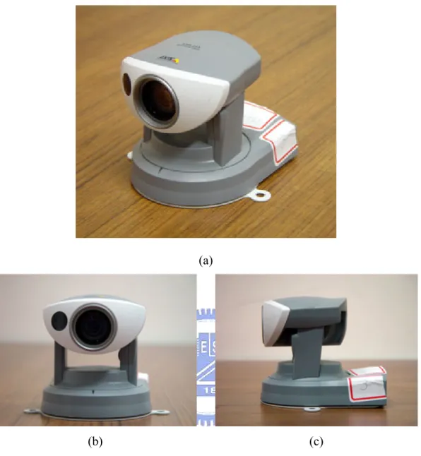
(24) Network cable. Laptop. Figure 2.1 Equipment connection situations in this study.. 2.2.1 Hardware configuration The hardware equipments we use in our system include three parts. The first part is a laptop which we use to run our program. A kernel program can be executed on the laptop to control the vehicle by issuing commands to the vehicle. It also can be used to get the status information of the vehicle. The second part is the vehicle which has an aluminum body. The size of it is 44cm×38cm×22cm with three wheels of the same diameter of 16.5cm. In the vehicle, there are three 12V batteries each of which, by one charge, supplies power to the vehicle to run 18-24 hours. The vehicle can reach a forward speed of 160cm per second and a rotation speed of 300 degrees per second. The embedded control system can be used to control the vehicle to move forward or backward and turn around by the user’s commands. The appearance of the vehicle is shown in Figure 2.2. The third part is a digital IP camera with panning, tilting, and zooming (PTZ) capabilities. The PTZ IP camera used in this study is an AXIS 213 PTZ made by AXIS, as shown in Figure 2.3. This is a camera with a height of 130mm, a width of 104mm, a depth of 130mm, and a weight of 700g. The pan angle range is 340 degrees and the tilt angle range is 100 degrees. It has 26x optical zooming and 12x digital. 12.

(25) zooming capabilities. The image captured in our experiments is of the resolution of 320×240 pixels for the reason of raising image processing efficiency. Moreover, the camera is directly connected to a laptop by a network cable for transmission of the captured image.. (b). (a). Figure 2.2 The vehicle Pioneer 3 used in this study. (a) A front view of the vehicle. (b) A side view of the vehicle.. 2.2.2 Software configuration The ActiveMedia Robotics provides an application interface ARIA to control the vehicle used in this study. ARIA is an object-oriented interface which is usable under Linux or Win32 in the C++ language and can dynamically control the velocity, heading, and other navigation settings of the vehicle. We use the ARIA to communicate with the embedded system of the vehicle. And we use the Borland C++ Builder as the development tool in our experiments. 13.

(26) (a). (b). (c). Figure 2.3 The pan-tilt-zoom camera used in this study. (a) A perspective view of the camera. (b) A front view of the camera. (c) A left-side view of the camera.. 2.3 Learning Strategy and Major Steps in Proposed Process The proposed learning strategy is based on human following [2]. When the vehicle follows a person, it uses the information of the clothes which the person wears. 14.

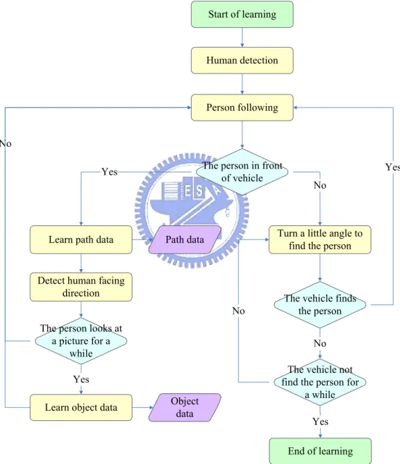
(27) Two kinds of situations should be handled. The first is that the vehicle can find the person by the clothes feature and the second is that the vehicle cannot find the person. In the first situation, the vehicle will keep following the person and avoid losing the observation of the person. In the second situation, the vehicle cannot follow the person anymore. Because the camera on the vehicle always pans to follow the person, the vehicle can keep knowing that the person is on which side with respect to the vehicle (left or right). If the person disappears in front of the vehicle, then the vehicle can find out the side on which the disappearing person was. After that, the vehicle will turn an angle to the correct its direction to search for the disappearing person in the acquired image. But if the vehicle turns for a pre-set number of times and still cannot find the person, then the system stops the learning strategy. Our system needs to learn two major kinds of data at the learning strategy. The first part is path data. These data are used in the path planning. The second part is the information of those objects which the person wants the vehicle to monitor. The person only needs to stand in front of the object and looks at it. Then the vehicle will go forward to learn the information of the object. These data are used in the patrolling process. The major steps are shown in Figure 2.4.. 2.4 Path Planning and Patrolling Principle and Major Steps in Proposed Process After the vehicle learns the path and the object data in the learning stage, the vehicle refines the path and stretches the rough part of the path by analyzing these 15.

(28) data using a binary-cut line fitting technique. The path planning process has three major steps. The first step is to retain the nodes where the monitored objects are located. After doing the first step, the path is separated into some segments. Then, we collect these path segments by pushing them into an empty queue.. Start of learning. Human detection. Person following No The person in front of vehicle. Yes. Learn path data. Yes No. Turn a little angle to find the person. Path data. Detect human facing direction No. The vehicle finds the person. The person looks at a picture for a while. No. Yes. The vehicle not find the person for a while. Learn object data. Object data. Yes End of learning. Figure 2.4 An illustration of the automatic learning process by person following.. 16.

(29) The second step that is to pop out one segment from the queue and check the segment to see whether it is smooth enough or not. If the answer is no, then go to the third step to separate the segment again into two small parts and push them into the queue mentioned before. We then execute the second step again and repeatedly, until the queue is empty. We save the segments which are smooth enough to be the path data, for use in the patrolling process. The major steps are illustrated in Figure 2.5. After doing the steps of the path planning, the next process is navigation to the start point. The navigation process includes three major steps. The first step is to read and sort the path data obtained from the path planning. The second step is to go forward according to the path data, and check the current position to see whether there is an object to be monitored there or not. If the answer is yes, then go to the third step to match the monitored object. We repeat the second and the third steps until the vehicle arrives at the start point. The major steps are illustrated in Figure 2.6.. 2.5 Vehicle Navigation Principle and Major Steps in Proposed Process Our system has two major processes in the vehicle navigation system. The first is the learning process. The vehicle learns the information of a navigation path in this process. We divide the navigation path into several segments, and the divided points are the positions where the vehicle needs to turn. Also, the vehicle needs to learn two kinds of major information of every segment of the navigation path. One is the information of the environment of the path where the vehicle navigates and the other is the information of a turning node which the vehicle passes by. The major steps are. 17.

(30) illustrated in Figure 2.7.. Start of path planning. Separate path and push path data into an empty queue. Object data. Get a part of path from queue. Point data. The part of path is smooth enough?. No. Separate the part of path into two part and push into queue. Yes Path data. Allow the part of path. If the queue is empty?. Yes End of path planning. Figure 2.5 An illustration of the path planning process.. The second part of our system is the navigation process. After reading the data of the navigation path which is separated into several segments by the turning nodes obtained from the learning process, the vehicle can now navigate and guide, if necessary, a visitor on the path, by performing two tasks at every segment. One is navigation in the middle of the hallway and the other is finding the position of the turning node. These major steps are illustrated in Figure 2.8. 18.

(31) Start of patrolling. Read and sort the path data Navigation to the next node. No. Original node?. Path data. No. Has monitored object data?. Yes. Yes. End of patrolling. Monitor object matching. Object data. No. Yes Adjust vehicle location. Figure 2.6 An illustration of the patrolling process. Start of learning. Learn hallway information Guiding path data No. Learn turning node information. Arrives the destination? Yes End of learning. Figure 2.7 An illustration of the learning process of the vehicle navigation system.. 19.

(32) Start of guiding. Guiding path data. Read path data. Navigate on the hallway No. No. Arrive at the turning node?. Yes Turn. Arrive at the destination?. Yes End of guiding. Figure 2.8 An illustration of the navigation process.. 20.

(33) Chapter 3 Camera and Odometer Calibration. 3.1 Introduction The camera and the odometer are the two important equipments of the vehicle used in this study. In this chapter, we describe the proposed calibration methods for these two equipments. Distance information is important and useful in the person following process. The vehicle of our system computes the distance information by analyzing images captured from the camera. But there is ambiguity in the inverse mapping from 2D image coordinates to 3D world positions. Wang and Tsai [1] proposed a method of angular mapping for camera calibration to compute the distance between a vehicle and a person. Chen and Tsai [9] proposed a method of area tracking to deal with the situation where the vehicle cannot see the entire clothes of the person. In Section 3.2, we will review these methods and propose another method which can improve the practicability of these camera calibration methods. For vehicle navigation in indoor environments, the vehicle location is the most important information to guide the vehicle in correct paths. Though the information provided by the odometer of the vehicle is precise enough for inferring the vehicle location for most applications, it cannot be used solely for the navigation process because the incremental mechanical errors might result in imprecise odometer data and so in deviations from the planned navigation path. Hence, in order to keep the navigation in track, a vision-based odometer calibration technique is desirable to 21.

(34) eliminate the errors. In Section 3.3, we will propose a technique for this purpose.. 3.2 Camera Calibration by Cross Shape Detection 3.2.1 Idea of Proposed Camera Calibration Method The distance information is indispensable for a person-following vehicle. The vehicle can avoid striking a person by using the distance information to keep a safe distance to the person. And the vehicle can go forward to see more clearly for avoiding losing information of this person by using the distance information when the person is far from the vehicle. Our system computes the distance information by analyzing the images captured from the camera. Through imaging with the camera, 3D world coordinate systems are mapped into 2D image coordinate systems. However, there is ambiguity in the inverse mapping from a 2D image point to its corresponding 3D world location because each point in the image is the projection result of a light ray onto the image sensor. The light ray can be described by a longitude angle and a latitude angle in the 3D world space. To define the corresponding longitude and latitude angles (or simply called longitude and latitude in the sequel) of each point in images, Wang and Tsai [1] proposed a method of 2D mapping to achieve the goal of angular-mapping camera calibration.. However, some steps repeat and incur error easily in their method. We will propose a method which simplifies the steps of camera calibration and is suitable for common users. In Section 3.2.3, we will review the method of angular-mapping. 22.

(35) camera calibration. In Section 3.2.4, we will describe the proposed method. Before describing the above-mentioned methods, we first introduce the definitions of the coordinate systems and the directional angle of the camera used in this study in Section 3.2.2.. 3.2.2 Coordinate Systems and Directional Angles of Camera Four coordinate systems are utilized in this study which describes the relative locations between the vehicle and encountered objects. The coordinate systems are shown in Figure 3.1. The definitions of all the coordinate systems are stated in the following. (1) Image coordinate system (ICS): denoted as (u, v). The uv-plane of the system is coincident with the image plane and the origin I of the ICS is placed at the center of the image plane. (2) Global coordinate system (GCS): denoted as (x, y). The x-axis and the y-axis are defined to lie to on the ground, and the origin G of the global coordinate system is a pre-defined point on the ground. In this study, we define G as the starting position of the person-following process. (3) Vehicle coordinate system (VCS): denoted as (Vx, Vy). The VxVy-plane is coincident with the ground. And the origin V is placed at the middle of the line segment that connects the two contact points of the two driving wheels with the ground. The Vx-axis of the system is parallel to the line segment joining the two driving wheels and through the origin V. The Vx-axis is perpendicular to the x-axis and goes through V. (4) Spherical coordinate system (SCS): denoted as (ρ, θ, φ). This system is proposed 23.

(36) by Wang and Tsai [1]. It is a 3D polar coordinate system and we explain this system in terms of the 3D Cartesian coordinate system with coordinates (i, j, k) for convenience. The origin S of the spherical system, which is also the origin of the Cartesian system, is the optical center of the camera. The ij-plane of the Cartesian system is parallel to the uv-plane in the ICS. A point P at coordinates (i, j, k) in the Cartesian space is represented by a 3-tuple (ρ, θ, φ) in the spherical space. The value ρ with ρ ≥ 0 is the distance between the point P and the origin S. The longitude θ is the angle between the positive k-axis and the line from the origin S to the point P projected onto the ik-plane. The latitude φ is the angle between the ik-plane and the line from the origin S to the point P.. Two kinds of directional angles of a camera are used in this study. One is the pan angle and the other the tilt angle. The pan angle of the camera is defined in the VCS, denoted by θc. It represents the degree of horizontal rotation of the camera and is important for coordinate transformation.. Room. w. I. u. y. G. (a). x. (b). Figure 3.1 The coordinate systems used in this study. (a) The image coordinate system. (b) The global coordinate system (c) The vehicle coordinate system. (d) The spherical coordinate system.. 24.

(37) Vy. Vx. (c) (d) Figure 3.1 The coordinate systems used in this study. (a) The image coordinate system. (b) The global coordinate system (c) The vehicle coordinate system. (d) The spherical coordinate system. (continued). We define the direction of the y-axis to be zero. The value of θc is exactly the angle between the camera direction and the direction of the y-axis. The range of θc is between 0 and π if θc is in the first and fourth quadrants and between 0 and –π if θc is in the second and third quadrants, as shown in Figure 3.2. The tilt angle of the camera is defined as the angle between the optical axis of the camera and the ground. The angle, denoted as φc, represents the vertical tilting of the camera. We define the angle to be zero when the optical axis of the camera is parallel to the ground. The range of φc is between 0 and π/2 if the camera tilts up, and is between 0 and –π/2, else, as. shown in Figure 3.3.. 3.2.3 Review of Adopted Camera Calibration Method Wang and Tsai [1] proposed a nonlinear angular mapping method to precisely obtain the angular transformation from the real world to the image. By the angular 25.

(38) information of the light rays and the height of the camera, we can know the relative distances of targets in images.. (b). (a). Figure 3.2 The pan angle of the camera. (a) 0 ≤ θ c ≤ π . (b) 0 ≥ θ c ≥ −π .. The coordinate system used in this method is shown in Figure 3.4, which includes the previously-mentioned image coordinate system (ICS) described by image coordinates (u, v) and the spherical coordinate system (SCS) described by parameters (ρ, θ, φ). The latter is a 3D polar coordinate system which can be explained in terms of the 3D Cartesian coordinate system with coordinates (i, j, k). The ij-plane of the Cartesian system is parallel to the uv-plane in the ICS. The origin S of the SCS, which is also the origin of the Cartesian system, is the optical center of the camera. A point P at coordinates (i, j, k) in the Cartesian space is represented by a 3-tuple (ρ, θ, φ) in the SCS where ρ is the distance between the point P and the origin S. The longitude θ is the angle between the positive k-axis and the line from the origin S to the point P projected onto the ik-plane, and the latitude φ is the angle between the ik-plane and the line from the origin S to the point P.. 26.

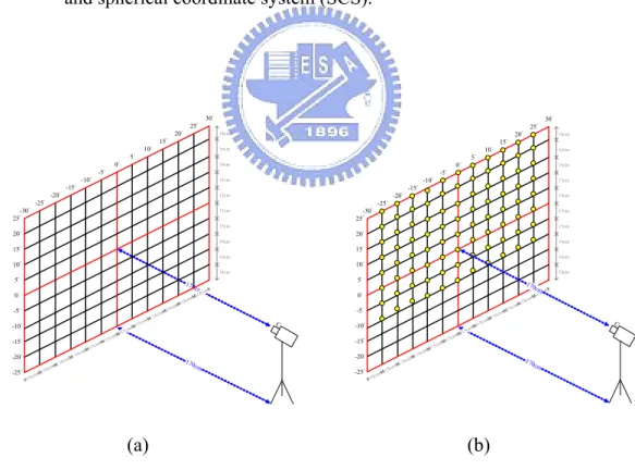
(39) p/2. p/2. fc. 0. 0 fc. -p/2. -p/2 (a). (b). Figure 3.3 The tilt angle of the camera. (a) 0 ≤ ϕ c ≤. π 2. . (b) 0 ≥ ϕ c ≥ −. π 2. .. A grid board is used in this method. It has m vertical lines and n horizontal lines, and is attached on a wall which is perpendicular to the ground. Because the longitude and the latitude values of the intersection points in the grid have been known in advance, the longitude and the latitude values of the other pixels in the image can be computed by an interpolation method. In this way, the longitude and the latitude values of each pixel in the image can be obtained. In Figure 3.5, we can see the respective positions of the grid board and the camera use in this method. And the views from the camera are shown in Figure 3.6. The intersections of the lines are marked by yellow points. After knowing the longitude and the latitude values of the yellow points in the image by previously-mentioned nonlinear angular mapping, we can use an interpolation method to compute the longitude and the latitude values of the other pixels in the image.. 27.

(40) Figure 3.4 An illustration of transformation between image coordinate system (ICS) and spherical coordinate system (SCS).. 30°. 30°. 25° 20°. 25° 20°. 18cm. 15°. 18cm. 15°. 10°. 10°. 16cm. 5°. 16cm. 5°. 0°. 0°. 16cm. -5°. 16cm. -5°. -10°. -10°. 15cm. -15°. 15cm. -15°. -20°. -20°. 15cm. -25°. 15cm. -25°. -30° 25°. -30° 25°. 15cm. 15cm. 15cm. 15cm. 20°. 20° 16cm. 16cm. 15°. 15° 16cm. 16cm. 10°. 10°. 18cm. 18cm. 5°. 170. 0° -5° -10° -15° -20° -25°. 18c. m. m 18c. 16c. m. m 16c. m 15c. m 15c. m 15c. 15c. m. m 16c. m 16c. 18c. m. 5°. cm. m 18c. 170 cm m c. 0° -5°. C. -10° -15°. 170. -20°. cm. -25°. (a). m 18c. m 18c. m 16c. m 16c. m 15c. m 15c. m 15c. m 15c. m 16c. m 16c. m 18c. 18. C. 170 cm. (b). Figure 3.5 Camera calibration by a vertical grid board. (a) An illustration of attaching the lines on the wall. (b) The intersections seen by camera are marked by yellow points.. 28.

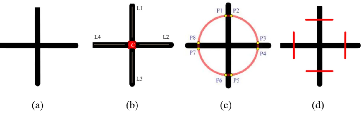
(41) (a). (b). Figure 3.6 The camera views of Figure 3.5. (a) View of Figure 3.5(a). (b) View of Figure 3.5(b).. 3.2.4 Proposed Cross Shape Detection Technique By using the camera calibration method which is mentioned in Section 3.2.2, we can convert the coordinate values of every pixel in the image coordinate system (ICS) into the spherical coordinate system (SCS). An important step is to mark the intersection points in an image of the grid board. However, it is required to point out every intersection point manually in this method. The work is repeated many times and is prone to incur errors. To deal with this problem, we propose a technique of cross shape detection which can be adopted to locate the intersection points in the image automatically. A look of a cross shape which has two lines intersecting each other is shown in Figure 3.7(a). For detecting the cross shape, we have to find out its property. A different definition of cross shape is a shape which has a center point C with four lines L1, L2, L3 and L4 emerging out of the center in four directions, as shown in Figure. 3.7(b). Let C denote the center. After we draw a circle, it can be divided into four. 29.

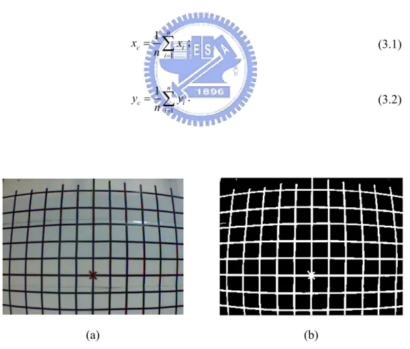
(42) curve parts, P1P2, P3P4, P5P6 and P7P8, intersecting the four lines of the cross shape respectively, as shown in Figure 3.7(c). By a careful observation around the circle, we can discover a common property of the eight intersection points, P1 to P8, that is, the positions of the eight points are located at places where the cross shape changes its color from white to black or from black to white. That means if we choose a point on the grid board randomly, let the point be the center to draw a circle, and find out the color changes eight times through the circle, then we can decide that the point is the center point of a cross shape. On the contrary, if we choose a point on the grid board randomly, let the point be the center to draw a circle, and find out that the color changing times are not equal to eight, then we can say that the point is not the center point of the cross shape. We can simplify this technique by using four lines instead of using the circle, as shown in Figure 3.7(d). That is, we check every point of the foreground on the grid board by using a matrix, which is shown in Figure 3.8, to scan the four lines composed of yellow cells and count the times of color changing. If the color of the grid board changes eight times, then we can decide C to be the center of the cross shape. The detailed process is described in the following as an algorithm. An experimental result of cross shape detection is shown in Figure 3.9. Figure 3.9 shows the image captured from the camera. Figure 3.9(b) is the thresholding result of Figure 3.9(a). In Figure 3.9(c), many groups of centers of cross shapes are detected. Figure 3.9(d) shows the final result in which the real center of every cross shape have been found out. We conducted the calibration work and saved the longitude and the latitude values of every pixel in the image into a bmp image as shown in Figure 3.9(e). Figure 3.10 shows the program windows for camera calibration.. 30.

(43) L1. L4. L2 C. L3. (a). (b). (c). (d). Figure 3.7 Detection of the cross point of a cross shape. (a) The look of a cross shape. (b) A center point and four lines composing the cross shape. (c) A circle with four intersections with the cross shape. (d) Use of four lines to detect the cross shape.. 1. .... 1 1. 1 C. 1. 1 1. .... 1. Figure 3.8 The matrix used to detect the cross shape.. Algorithm 3.1. Computing the intersection points in a calibration target image. Input: An image taken from camera Ic, and the gray version Ig of Ic. Output: A set S of intersection points of the image Ic, with coordinates (xc1, y c1), (xc2, y c2), …, (xcn, y cn) Steps:. Step 1. Calculate a threshold value T of the gray value which can differentiate the background and the foreground of Ic. 31.

(44) Step 2. Reset the gray value gpi of every pixel pi in the image Ig in the following way: If gpi > T is satisfied, set gpi as a foreground point; else, if gpi ≤ T is satisfied, set gpi as a background point. Step 3. Calculate the times ti of color changing around every pixel of the foreground. Step 4. Delete the point pi whose value ti is not equal to eight, and consider the remaining points as centers. Step 5. Calculate the centroid of every group of centers and find out the intersection points by Eqs. (3.1) and (3.2) below:. xc =. 1 n ∑ xi ; n i =1. (3.1). yc =. 1 n ∑ yi . n i =1. (3.2). (a). (b). Figure 3.9 Some experimental results of cross shape detection. (a) Original Image. (b) After thresholding. (c) Find groups of centers. (d) Center detected. (e) The bmp image with camera calibration information. 32.

(45) (c). (d). (e) Figure 3.9 Some experimental results of cross shape detection. (a) Original Image. (b) After thresholding. (c) Groups of centers detected. (d) Centers detected. (e) The bmp image with camera calibration information. (continued). Figure 3.10 The program window of camera calibration.. 33.

(46) 3.3 Odometer Calibration by Quadratic Functions 3.3.1 Idea of Odometer Calibration The vehicle moving direction is another important information factor for guiding the vehicle to navigate in indoor environments. The direction information is provided by the odometer of the vehicle. However, the vehicle cannot navigate by using the odometer information only because the incremental mechanical errors might result in imprecise odometer data. Hence, in order to keep the navigation in the path, odometer calibration must be carried out to eliminate the errors. The vehicle we use in this study has mechanical errors, as mentioned. It deviates gradually to left when it moves forward on a straight line, as observed in our experiments. In this study, we propose a technique to collect the data of the deviation, and analyze the data to build an odometer calibration model. In Section 3.3.2, we will describe the details of the odometer calibration model we adopt which can eliminate the mechanical errors. After finding out the deviation values in every different distance, we want to apply this model to compute the deviations of all distances by a curve fitting scheme which we will discuss in Section 3.3.3. The use of such calibration results is described in Section 3.3.4.. 3.3.2 Odometer Calibration Model Before building an odometer calibration model, we prepare some equipment for our experiment. We use a sticky tape, a measuring tape, an autonomous land vehicle, and a computer. First, we fix the initial position O of the vehicle and mark the position 34.

(47) by pasting a sticky tape on the ground. Second, we fix the initial direction of the vehicle and paste a straight line L along the direction on the ground by using a stick tape. Third, we send commands to drive the vehicle forward on a straight line, and then commands to stop the vehicle. Fourth, we mark the terminal position T of the vehicle by pasting a piece of sticky tape on the ground. Fifth, we find the node P on the straight line L which is the vertical projection of the terminal position T. Sixth, we measure the distance D1 between O and T which is the move distance of the vehicle, and the distance D2 between T and P which is the deviation produced by mechanical errors. Seventh, we compute the angle Θ of the inverse sine value of D2/D1 which is the angle of the deviation. We repeat the steps at least twenty times and let the distance the vehicle moves be different every time. An illustration of the experiment is shown in Figure 3.11. The resulting values are shown in Table 3.1 and the distribution of the results is shown in Figure 3.12.. Algorithm 3.2. Building an odometer calibration model. Input: None. Output: An odometer calibration model. Steps:. Step 1.. Fix the initial position O and initial direction line L of the vehicle.. Step 2.. Send commands to let the vehicle move forward and then stop.. Step 3.. Mark the terminal position T of the vehicle.. Step 4.. Find the vertical projection node P of the terminal position T of the vehicle on the straight line L.. Step 5.. Measure the distance D1 between O and T and the distance D2 between T and P.. 35.

(48) Step 6.. Compute the angle Θ of inverse sine value of D2/D1.. Step 7.. Repeat Step 1 to Step 6 at least twenty times and let the distance the vehicle moves every time be different.. Figure 3.11 An illustration of the experiment.. Relation of Move Distance and Angle of Departure 10 9 Angle of Departure. 8 7 6 5 4 3 2 1 0 0. 100. 200. 300. 400. 500. 600. 700. Move Distance (cm). Figure 3.12 The distribution of the angles of the deviations. 36.

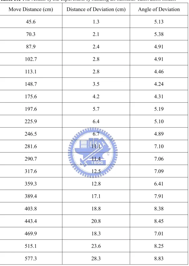
(49) Table 3.1 The results of the experiment of building an odometer calibration model.. Move Distance (cm). Distance of Deviation (cm). Angle of Deviation. 45.6. 1.3. 5.13. 70.3. 2.1. 5.38. 87.9. 2.4. 4.91. 102.7. 2.8. 4.91. 113.1. 2.8. 4.46. 148.7. 3.5. 4.24. 175.6. 4.2. 4.31. 197.6. 5.7. 5.19. 225.9. 6.4. 5.10. 246.5. 6.7. 4.89. 281.6. 11.1. 7.10. 290.7. 11.4. 7.06. 317.6. 12.5. 7.09. 359.3. 12.8. 6.41. 389.4. 17.1. 7.91. 403.8. 18.8. 8.38. 443.4. 20.8. 8.45. 469.9. 18.3. 7.01. 515.1. 23.6. 8.25. 577.3. 28.3. 8.83. 3.3.3 Curve Fitting After measuring the values of the angles of deviations, we found out that the 37.

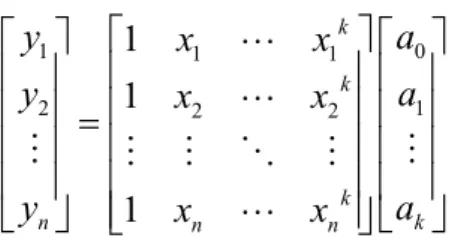
(50) distribution of data has a trend which may be roughly described as a curve of the second order with respect to the vehicle move distance value. Therefore, we use a least squares error (LSE) fitting method to fit the data with a curve. And then we can use the resulting curve for odometer calibration while patrolling. The method is explained as follows. First, we generalize a straight line to a curve of the kth-degree polynomial:. y = a 0 + a 1 x + ... + a k x k ,. (3.3). with the residual given by n. [ (. R ≡ ∑ y i − a 0 + a1 xi + ... + a k x i 2. i =1. )] .. (3.4). )]. (3.5). 2. k. The partial derivatives of R2 are. ( ). [ (. n ∂ R2 = −2∑ y − a 0 + a1 x + ... + a k x k = 0 ; ∂a 0 i =1. ∂ ( R2 ) ∂a1 ∂ ( R2 ) ∂ak. n. = −2∑ ⎡⎣ y − ( a0 + a1 x + ... + ak x k ) ⎤⎦ x = 0 ;. (3.6). i =1. n. = −2∑ ⎡⎣ y − ( a0 + a1 x + ... + ak x k ) ⎤⎦ x k = 0 .. (3.7). i =1. These lead to the following equations: n. n. n. i =1. i =1. i =1. a0 n + a1 ∑ xi + ... + ak ∑ xik = ∑ yi ;. n. n. n. n. i =1. i =1. i =1. i =1. a0 ∑ xi + a1 ∑ xi2 + ... + a k ∑ xik +1 = ∑ xi yi ;. 38. (3.8). (3.9).

(51) n. n. n. n. i =1. i =1. i =1. i =1. . a0 ∑ xik + a1 ∑ xik +1 + ... + a k ∑ xi2 k = ∑ xik y ,. (3.10). or, in matrix form,. ⎡ ⎢ n ⎢ ⎢ n ⎢ ∑ xi ⎢ i =1 ⎢ ⎢ n ⎢∑ x k ⎢⎣ i =1 i. n. ∑x. i. i =1 n. ∑x. 2. i. i =1. n. ∑x. k +1. i. i =1. ⎤ ⎡ n ⎤ … ∑ xi ⎥ ⎢ ∑ yi ⎥ i =1 ⎥ ⎡ a0 ⎤ ⎢ i =1 ⎥ n ⎢ n ⎥ ⎥ k +1 ⎥ ⎢ … ∑ xi ⎥ ⎢ a1 ⎥ ⎢ ∑ xi yi ⎥ = i =1 ⎥ ⎢ ⎥ ⎢ i =1 ⎥. ⎥⎢ ⎥ ⎢ ⎥ a ⎥ ⎢ ⎥ k ⎣ ⎦ n n 2k ⎥ k ⎥ ⎢ xi y … ∑ xi ⎥⎦ ⎢⎣ ∑ ⎥⎦ i =1 i =1 n. k. (3.11). This is a Vandermonde matrix. We can also obtain the matrix for a least squares fit by writing:. ⎡1 x1 ⎢ ⎢1 x2 ⎢ ⎢ ⎢⎣1 xn. x1k ⎤ ⎡ a0 ⎤ ⎡ y1 ⎤ ⎥⎢ ⎥ ⎢ ⎥ x2 k ⎥ ⎢ a1 ⎥ ⎢ y2 ⎥ = ⎥⎢ ⎥ ⎢ ⎥. ⎥⎢ ⎥ ⎢ ⎥ xn k ⎥⎦ ⎣ ak ⎦ ⎣ yn ⎦. (3.12). Pre-multiplying both sides by the transpose of the first matrix then gives ⎡1 ⎢x ⎢ 1 ⎢ ⎢ k ⎣ x1. 1 ⎤ ⎡1 x1 ⎢ xn ⎥⎥ ⎢1 x2 ⎥⎢ k⎥⎢ xn ⎦ ⎢⎣1 xn. 1 x2 x2 k. x1k ⎤ ⎡ a0 ⎤ ⎡ 1 ⎥⎢ ⎥ ⎢ x2 k ⎥ ⎢ a1 ⎥ ⎢ x1 = ⎥⎢ ⎥ ⎢ ⎥⎢ ⎥ ⎢ k xn k ⎥⎦ ⎣ ak ⎦ ⎣ x1. 1 x2 x2 k. 1 ⎤ ⎡ y1 ⎤ xn ⎥⎥ ⎢⎢ y2 ⎥⎥ . ⎥⎢ ⎥ ⎥⎢ ⎥ xn k ⎦ ⎣ yn ⎦. (3.13). So, we have ⎡ ⎢ n ⎢ ⎢ n ⎢ ∑ xi ⎢ i =1 ⎢ ⎢ n ⎢∑ x k ⎢⎣ i =1 i. n. ∑ xi i =1 n. ∑x i =1. n. ∑x i =1. 2. i. i. k +1. ⎡ n ⎤ k ⎤ x ∑ i ⎥ ⎢ ∑ yi ⎥ i =1 ⎥ ⎡ a0 ⎤ ⎢ i =1 ⎥ n ⎢ n ⎥ ⎥ k +1 ⎥ ⎢ … ∑ xi ⎥ ⎢ a1 ⎥ ⎢ ∑ xi yi ⎥ . = i =1 ⎥ ⎢ ⎥ ⎢ i =1 ⎥ ⎥⎢ ⎥ ⎢ ⎥ a ⎥ ⎢ ⎥ k ⎣ ⎦ n n 2k ⎥ k ⎥ ⎢ … ∑ xi xi y ⎥⎦ ⎢⎣ ∑ ⎥⎦ i =1 i =1 …. n. (3.14). As before, given n points, a fitting of them with polynomial coefficients a0, a1, ..., 39.

(52) ak gives. ⎡ y1 ⎤ ⎡1 x1 ⎢y ⎥ ⎢ ⎢ 2 ⎥ = ⎢1 x2 ⎢ ⎥ ⎢ ⎢ ⎥ ⎢ ⎣ yn ⎦ ⎣⎢1 xn. x1k ⎤ ⎡ a0 ⎤ ⎥⎢ ⎥ x2 k ⎥ ⎢ a1 ⎥ ⎥⎢ ⎥. ⎥⎢ ⎥ xn k ⎦⎥ ⎣ ak ⎦. (3.15). In matrix notations, the equation for a polynomial fit is given by. Y = XA .. (3.16). This can be solved by pre-multiplying by the matrix transpose as follows:. X T Y = X T XA .. (3.17). This matrix equation can be solved numerically, or can be inverted directly if it is well formed, to yield the solution vector:. A = ( X T X ) −1 X T Y .. (3.18). The result of curve-fitting of the previously-mentioned set of angle data of deviations is shown in Eq. (3.19) below and illustrated in Figure 3.13.. f ( x) = 0.00000476 × x 2 + 0.00592048 x + 4.16437951 .. Figure 3.13 The results of line fitting of the angle of deviation.. 40. (3.19).

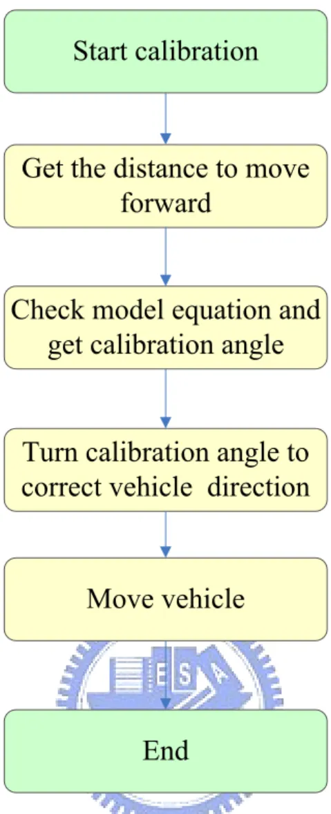
(53) 3.3.4 Navigation by Odometer Calibration In Section 3.3.2 and Section 3.3.3, we have described the process of building the odometer calibration model and found a quadratic function which can show the relationship between the distance the vehicle moves and the angles of deviations caused by the mechanical errors. In this section, we describe the process about using the quadratic function to calibrate the odometer while navigating the vehicle in indoor environment. We guide the vehicle most of the time while navigation by the command: “move to front.” But the vehicle always has a leftward deviation while moving forward. To deal with this problem, we use the odometer calibration model to balance the deviation. First, we have to know the distance D we want the vehicle to move forward. Second, we substitute the value D into Eq. (3.19) to get the angle of deviation Θ. That means if we command the vehicle to move to D centimeters ahead of the original position, then the vehicle should be instructed to deviate rightward for the angle of. Θ. Therefore, we issue a command of right turn of angle Θ before commanding the vehicle to move forward. In this way, we can balance the deviation. The major steps are shown in Figure 3.14.. 41.

(54) Start calibration. Get the distance to move forward. Check model equation and get calibration angle. Turn calibration angle to correct vehicle direction. Move vehicle. End. Figure 3.14 An illustration of odometer calibration.. 42.

(55) Chapter 4 Learning Procedures. 4.1 Introduction In this chapter, we introduce the details of the proposed learning procedures. Two kinds of environment features are used for learning in this study. The first is path data. In the procedures, the vehicle learns path data while following a person. An adopted method and an improved method of human following are described in Section 4.2. In Section 4.3, we describe how to gather path data when the vehicle follows a person in an indoor environment. The second feature is 2D object. In the learning procedures, the vehicle learns 2D objects if it detects the situation that the person stops and faces to the left or right side. An adopted method and an improved method of human facing direction detection are described in Section 4.4. For object monitoring, how to detect the 2D object automatically is the key issue, and we propose a method for it in Section 4.5. An illustration of the learning procedures is shown in Figure 4.1.. 4.2 Human Following 4.2.1 Review of Adopted Method Wang and Tsai [1] proposed a person following method which can conduct a 43.

(56) work of following a specified person by motion analysis of human clothes. The system user learned the clothes of the target person manually. The user decided the start point and the boundary box in the image for region growing of the clothes. After learning the image part of the person’s clothes, the system will enter the human tracking process. The major steps are shown in Figure 4.2.. Start of learning Following Human detection. Person following. The person still in front of vehicle?. No. Person tracking strategy. Yes. Learning path data. Path data. Human facing direction detection. The person stops and faces to lateral side. No. Yes Learning object data. Object data. Learning. Figure 4.1 An illustration of proposed learning procedures.. To detect the location of the target person by clothes, the system uses a clothes 44.