全域照明中結合模糊陰影與影像平面光子映射技術之研究

國立交通大學

多媒體工程研究所

碩 士 論 文

全域照明中結合模糊陰影與影像平面光子映射技術

之研究

Combining Soft Shadow and Image Space Photon Mapping for

Global Illumination.

研 究 生：姚人豪

指導教授：施仁忠 教授

全域照明中結合模糊陰影與影像平面光子映射技術之研究

Combining Soft Shadow and Image Space Photon Mapping for Global

Illumination

研究生：姚人豪

Student: Ren-Hao Yao

指導教授：施仁忠

Advisor: Zen-Chung Shi

國 立 交 通 大 學

多 媒 體 工 程 研 究 所

碩 士 論 文

A Thesis

Submitted to Institute of Multimedia Engineering College of Computer Science

National Chiao Tung University in partial Fulfillment of the requirements

for the Degree of Master

in

Computer Science

June 2011

Hsinchu, Taiwan, Republic of China

I

全域照明中結合模糊陰影與影像平面光子映射技術之研究

研究生: 姚人豪

指導教授

:

施仁忠 教授

國立交通大學多媒體工程研究所

摘 要

即時的全域照明技術在電腦圖學領域中，一直是一門重要的課題。過去受限於硬體 的計算能力,運用於遊戲或動畫中的渲染技術往往必須在速度與畫質之間作取捨；但隨 著繪圖處理單元(GPU)的進步，使用繪圖硬體為基礎的渲染演算法將成為即時渲染的關 鍵。 本篇論文提供了一個新的以繪圖硬體為基礎的即時全局照明演算法，他是結合了影 像平面光子映射(Image space photon mapping)以及其他模糊陰影的技術。藉由化簡光子 散射的步驟以及使用影像平面的模糊陰影演算法，我們改進了原有影像平面光子映射的 繪圖品質，並保有即時繪圖的演算速度。另外我們也使用泛用型光線追蹤引擎(Nvidia Optix)來讓所有的演算步驟都在繪圖硬體上執行。我們經由實作證明本演算法能夠支援 多種光學現象的結果，像是間接照明以及折射光的聚焦，並且能以即時的速度描繪。

II

Combining Soft Shadow and Image Space Photon Mapping

for Global Illumination.

Student: Ren-Hao Yao

Advisor: Dr. Zen-Chung Shih

Institute of Multimedia Engineering

National Chiao-Tung University

ABSTRACT

Real-Time global illumination in computer graphic is a very important topic. With the enhancement of GPU architectures in recent years, GPU-based rendering algorithms have become the key to perform high quality images in real time.

In this thesis, we propose a GPU-based real-time global illumination algorithm by combining image space photon mapping and other soft shadow effects. We simplify the photon splatting phase by using photon quads instead of photon volumes, and use image space soft shadow algorithm to improve image quality while preserving real-time rendering speed. Moreover, photon tracing is implemented by using Nvidia Optix ray tracing engine. Our system runs totally on the GPU, and can handle most optical phenomena, such as indirect lighting and caustics. We demonstrate that the results can be displayed at real-time frame rates.

III

Acknowledgements

First of all, I would like to express my sincere gratitude to my advisor, Pro. Zen-Chung Shih for his guidance and patience. Without his encouragement, I would not complete this thesis. Thank also to all the members in Computer Graphics and Virtual Reality Laboratory for their reinforcement and suggestion. Thanks for those people who have supported me during these days. Finally, I want to dedicate the achievement of this work to my family and the natural beauty around daily life.

IV

Content

摘 要 ... I ABSTRACT ... II Acknowledgement ... III Content ... IV List of Figures ... V List of Tables ... VII

Chapter 1 Introduction ... 1

1.1 Motivation ... 1

1.2 System Overview ... 2

Chapter 2 Related Work ... 4

2.1 Photon Tracing ... 4

2.2 Virtual Point Light ... 4

2.3 GPU-based Photon Mapping ... 5

2.4 Soft Shadow and Ambient Occlusion ... 6

Chapter 3 Algorithm ... 7

3.1 Initial Data ... 8

3.2 Photon Tracing ... 9

3.3 Photon Splatting ... 10

3.4 Image Space Soft Shadow ... 15

3.5 Image Space Radiance Interpolation ... 16

Chapter 4 Implementation Details ... 19

Chapter 5 Results and Discussion ... 21

Chapter 6 Conclusion and Future Work ... 29

V

List of Figures

Figure 1.1: Quality compare of ISPM[12] and ISM[16] ... 1

Figure 1.2: System Overview ... 3

Figure 2.1: Ambient Occlusion Volumes[8] ... 7

Figure 3.1: Eye's G-buffe... 8

Figure 3.2: Light's view G-buffer ... 8

Figure 3.3: Eye's view shadow map ... 9

Figure 3.4: Bad estimator of photons ... 11

Figure 3.5: Over shaded of icosohedron ... 11

Figure 3.6: Render photon centers as point. ... 12

Figure 3.7: Photon quad ... 13

Figure 3.8: Photon splatting with attenuation energy ... 14

Figure 3.9: Splatting result (indirect lighting only) ... 14

Figure 3.10: Image space gathering ... 15

Figure 3.11: The result without and with soft shadow ... 16

Figure 3.12: Result of subsampling and bilinear weighting ... 17

Figure 3.13: Result after normal and depth weighting ... 18

Figure 3.14: Final result(1x1 sampling) ... 18

Figure 4.1: Optix data structure ... 20

Figure 5.1: Cornell box scene ... 21

Figure 5.2: Happy buddha scene ... 23

Figure 5.3: Chinese dragon scene ... 22

Figure 5.4: Glass sphere scene ... 23

VI

Figure 5.6: Sibenik Scene ... 24

Figure 5.7: Sponza Atrium scene ... 24

Figure 5.8: Compare cornell box result ... 27

VII

List of Tables

Table 1: Detail performance statistic for scenes. ... 25 Table 2: Compare performance for scenes. ... 26

1

Chapter 1

Introduction

1.1 Motivation

Real-time global illumination in dynamic scenes is still a big challenge in computer graphics today. The performance of conventional rendering algorithms in computer games and animations is limited by the computing power of devices, and we are forced to trade rendering quality for speed. However, with the enhancement of GPU architectures in recent years, parallel rendering algorithms have become the key to perform high quality images in real time.

Among various effects of global illumination, indirect lighting and soft shadows are the two major factors of how lights influence a scene to produce photo-realistic results. In fact, they are natural phenomena in our daily life. Although indirect lighting is usually handled by ray tracing, traditional physically accurate ray tracing methods may cost tens of hundreds of minutes to render an image frame. Due to the high computation cost, indirect lighting is still a challenging topic in global illumination. Up to now, there are still many studies focusing on this problem.

Photon mapping [6] is an approach which can handle most optical phenomena such as indirect lighting and caustic. However conventional photon mapping algorithms need final gathering, which is the bottleneck of the whole process. Therefore, Image space photon mapping (ISPM) [12] combines reflective shadow map[3] and photon volume splatting to

2

solve this issue. Although ISPM applies splatting instead of gathering and exploits GPU to achieve high rendering speed, most of space in ISPM focuses on the light bounce estimation, but omit the realistic of shadow effect. Most shadow edges remain sharp, making the result unrealistic.

The goal of this thesis is to get more realistic results in real time by combining ISPM and other soft shadow methods. In our proposed approach, we simplify the ISPM and take

advantage of the information in reflective shadow maps. Our algorithm has the following main contributions：

1. We extend the original ISPM by combining soft shadow effects. 2. Simplify the implementation of the photon scattering phase of ISPM.

3. Reduce the number of passes of our algorithm by reusing G-buffer data and combining the final up-sampling pass into the soft shadow pass.

4. We implement our algorithm entirely on the GPU and avoid copying memory data between the CPU and the GPU.

5. Propose a new global illumination algorithm that considers soft shadow and indirect lighting.

Figure 1.1 (a) ISPM[12] result with sharp shadow edge. (b) Imperfect shadow map[16] result with lower rendering speed.

3

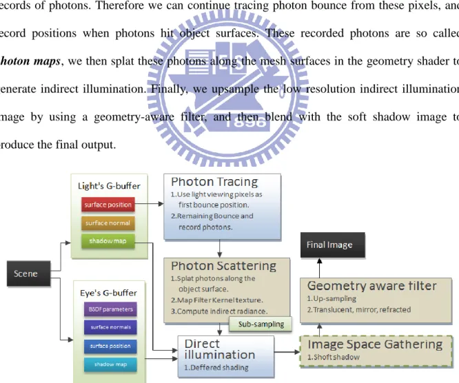
1.2 System Overview

An overview of our proposed rendering architecture is shown in Figure 1.2. Our method is a multi-pass rendering algorithm implemented entirely on GPU. First, we rasterize the scene from eye view and light view to produce images stored in buffers that we need in subsequent passes. These image buffers are called Geometry buffer (G-buffer)[18], which can be reused many times in subsequent passes. The eye's G-buffer is then used to produce direct illumination of a scene with deffered shading. Next, we use image space blurring techniques, with 3D geometry information in the image buffer, to produce soft shadow. Then, the light view surface pixels with position information can be regarded as the first bounce position records of photons. Therefore we can continue tracing photon bounce from these pixels, and record positions when photons hit object surfaces. These recorded photons are so called

photon maps, we then splat these photons along the mesh surfaces in the geometry shader to

generate indirect illumination. Finally, we upsample the low resolution indirect illumination image by using a geometry-aware filter, and then blend with the soft shadow image to produce the final output.

4

Chapter 2

Related Works

Global illumination is a widely studied and long developed research topic. A fundamental difficulty in global illumination is the high computation cost incurred by indirect lighting. Here we briefly review related work of indirect lighting. Besides, some soft shadow researches are also mentioned in this chapter.

2.1 Photon Tracing

The concept of tracing photons forward from the light source into the scene was introduced to the graphics community by Appel[1]. With similar concept, Jensen[6] introduced photon mapping. Conventional photon mapping has three major steps. First, shoot photons from the light source. Second, tracephotons forward from lights and store them in a k-d tree. Third, produce an image by tracing eye rays backwards and gathering nearby photons to approximate illumination where each ray intersects the scene. To reduce the final gathering step's expensive cost, many variations of photon mapping have been proposed.For example, Ma and McCool[10] use a hash grid rather than a k-d tree to store the photons.

2.2 Virtual Point Light

Another photon tracing family methods called virtual point light (VPL)[7]. Those VPLs are emitted from light sources, bouncing off surfaces according to material reflectance properties. Then render the scene lit by each VPL. Note that the VPL method is different from the photon mapping approach. Each VPL can influence the entire scene but photon mapping

5

are just a set of incident illumination. When scenes contain many thin parts or holes, the illumination effects such as caustics, cannot be adequately captured by using a small number of VPLs.

Reflective shadow map[3] treats each viewing pixel from light source as a VPL. Then compute the contribution of each surface normal while ignore the occlusion of objects. Imperfection shadow map[16] bases on the observation that shadows caused by indirect lighting more blurred. So they render low resolution shadow map from each VPL, and use pull-push to fill holes of coarse shadow map. Then use these imperfect shadow maps to solve the occlusion problem of traditional VPL. Micro-Rendering [15] represents scene's surface by hierarchical point-base scene representation, and projects these points onto each viewing position to obtain indirect lighting information.

Although previous works can provide almost photo-realistic effect, but can only support once bouncing itself. In contrast, our method can handle multiple bounces without any pre-computation.

2.3 GPU-based Photon Mapping

With the rapidly increasing computation power of modern GPUs, recent works are focused on GPU-based solutions for global illumination. Purcell et al.[14] implement the first GPU-based photon mapping. Wang et al.[19] exploit GPU-based photon mapping, by approximating the entire photon tree as a compact illumination cut, then cluster visible pixels and apply final gathering only on the clustering center pixels, to reduce the cost of gathering.

6

splatting [5], instead of gathering radiance from nearby photons, they scatter radiance from photons to nearby pixels. ISPM uses photon volume to represent the regain that the photon would be influenced. Then use rasterization to obtain pixels influenced by each photon. Although ISPM uses multi-core CPU to compute photon tracing, the cost of photon tracing procedure is still the bottleneck of performance. NVidia Optix[13] is a general purpose ray tracing engine based on NVIDIA® CUDA™ and other highly parallel architectures. Although Optix improves the tracing speed of ISPM, the Optix ISPM implementation still remain sharp shadow edge. In order to combine with other soft shadow algorithm, we use our own implementation of ISM while remains using Optix for the photon tracing procedure.

2.4 Soft Shadow and Ambient Occlusion

Conventional soft shadow and ambient occlusion [9] effects are accurately computed by using distributed ray tracing[2]. However, it is expensive, requiring tens to hundreds of rays per pixel. Ambient Occlusion Volumes (AOV)[8, 11] has similar concept as shadow volume. They use volume to compute the accessibility of each triangle in a scene. It has the same idea as the ISPM, by using rasterization to accelerate computation. In our experiments, the covered range of volume needed to rasterdetermines the fps of performance. As a result, we use image space soft shadow method to reduce the cost of GPU shading. Such as percentage-closer soft shadow (PCSS)[4] and image space gathering (ISG)[17].

7

Chapter 3

Algorithm

In this thesis, we proposed an approach to enhance the algorithm of McGuire and Luebke [11]. The enhancement simplifies the photon splatting phase and considers the soft shadow effect. The steps of our algorithm are below, note that all steps take place on the GPU. For each frame we perform :

1. Render G-buffers from each light's view. 2. Render G-buffer from eye's view.

3. Trace shadow map from eye's viewing world position map. (Use Opitx) 4. Trace photons from light's viewing world position map, and record bounced

photons in photon maps. (Use Optix)

5. Render indirect lighting by splatting photons, stored in photon map. 6. Render direct lighting with soft shadow by using image space gathering.

7. Up-sample indirect illumination by geometry filter and blend with direct lighting result.

The rest of this chapter is organized as follows. In Section 3.1, we show the initial data we need, and data structures of photon. In Section 3.2, we describe the photon tracing and Section 3.3 for photon splatting. In Section 3.4 we describe how we generate soft shadow by deffered shading and image space gathering. And in Section 3.5 we describe the up-sampling and geometry filter method.

8

3.1 Initial Data

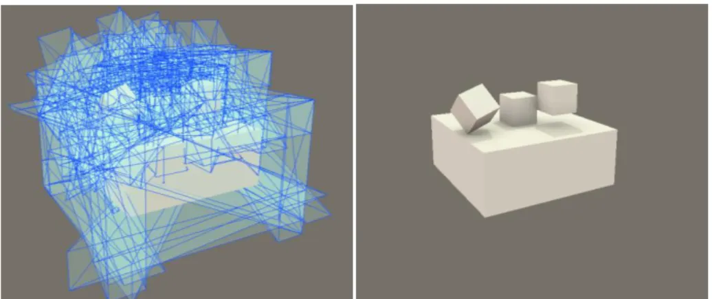
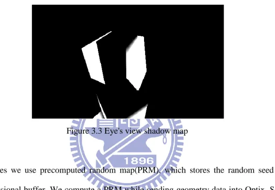
We first render the scene from eye's view to produce an eye's G-buffer, as shown in Figure 3.1. The eye's G-buffer contains the 3D information of each visible pixel, including world space position, world space normal, depth and flux. The light's G-buffers, as shown in Figure 3.2, are image data rendered from spot light source with emitted direction. We then trace rays from eye's world position map to produce shadow map, as shown in Figure 3.3. Note that all our tracing steps take place in GPU by using Nvidia Optix[13]. We pass G-buffer data to Optix by using openGL pixel buffer object(PBO).

Figure 3.1 Eye's G-buffer (a) world-space positions and (b) normal vectors(c) original eye view.

9

We trace rays from each light's viewing pixel, and record photons of each bounce until reaching the maximum bouncing times. In order to record photons on object surface, we allocate one-dimensional buffer called photon map. The size of photon map is the resolution of the light's G-buffer plus the max bouncing times. In each photon record, we store : photon position, normal to surface hit, photon power and path density. The path density is used to scale the splatting radius. So we can get more details in caustic regions.

Figure 3.3 Eye's view shadow map

Besides we use precomputed random map(PRM), which stores the random seed in a two-dimensional buffer. We compute a PRM while sending geometry data into Optix. So we only compute it once. Then we reuse this PRM while bounce incurred.

3.2 Photon Tracing

The light 's G-buffer represents the first bounce of ray casting. So after photons emit from each light source, we continue tracing photons from light's G-buffer pixels. By using the information stored in each pixel (ex: world position, normal, flux), we can compute the new direction of rays after bouncing. Then trace rays along these new directions. When a ray intersects the scene, we record the photon data in photon map. For point light source, we can use a six-view G-buffer cube map or just discard the light's G-buffer. Since Optix already

10

have all geometry information, we can emit photon from two hemisphere which cover the point light. Then trace and bounce each photon, and just record photons bouncing more than twice. Because the first bounce contribution are computed by direct lighting with deffered shading. Then we use those recorded photon to splat indirection illumination later.

While ray hit a diffuse surface, we compute new bouncing direction by random select a sample from hemisphere toward outside of the surface point itself. This random number is stored in PRM we mention in Section 3.1. For reflection material we use incident vector and surface normal to compute reflective direction. For glossy objects we take the average of diffuse and reflection directions.

3.3 Photon Splatting

Conventional photon mapping computes visible pixel radiance by gathering nearby photons. A photon is described by world space position. In order to obtain nearby photons of a specific position efficiently, photons are linked in k-d tree, called photon map[6]. Although k-d tree speeds up the searching of nearby photons, the gathering step of traditional photon mapping is still time consuming. Instead of using gathering, we estimate radiance by scattering radiance from photons to nearby pixels. Additionally, we apply weights to their contribution by using the same filter kernel as traditional photon gathering.

Image space photon mapping(ISPM)[12] uses icosohedron to bound the region influenced by photons. ISPM calls this icosohedron as photon volume. They compress these photon volumes along the surface normal. So they can abstain bad estimator such as the back faces of a thin object.

11

Figure 3.4 Bad estimator of photons mention in ISPM[12]

Instead of ISPM using compressed icosohedron as photon volume, we splat each photon along a surface as a quad which is strutted by two triangles. This simplification has two advantages. First, the fewer triangle we need to raster. Second, in order to avoid bad estimator(as shown in Figure 3.4 ), ISPM compressed icosohedron on the object surface, the 2D quad can avoid bad estimator, too.

For each pixel covered by photon quad, we compute the photon's incremental contribution as follows：

L(s ) = f(s ) ∗ (n ∙ np ) ∗ Φp∗ κ(s − s ) p (1)

Where s is the position of the shading pixel, n is the shading pixel's normal, s and _p np

are photon position and normal, Φp is the power of photon, f(s ) is the surface material

12

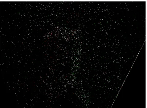
Figure 3.6 Render photon centers as point.

We send photons recorded in photon map into vertex shader as points. Figure 3.6 shows result of rendering photons as point data. We cull those back facing photons by dot product of eye direction and photon normal. Because these photons do not contribute to visible pixels. Next, we send photons into geometry shader for spaltting. In geometry shader, we generate photon quad by photon position and photon normal. It can be done by four predication as shown below： if(worldNormal.x==0){ offset.x=1; offset.y=0; offset.z=0; } else if(worldNormal.y==0){ offset.x=0; offset.y=1; offset.z=0; } else if(worldNormal.z==0){ offset.x=0; offset.y=0; offset.z=1; } else{ offset.x=0; offset.y=worldNormal.z; offset.z=-worldNormal.y; }

13

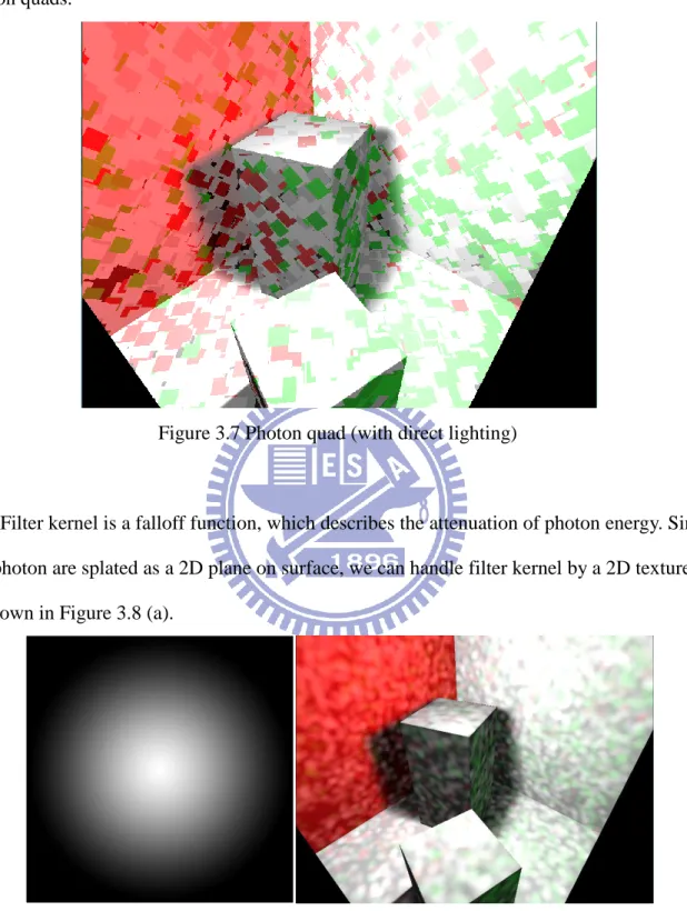
generate four new vertices at each photon point. Figure 3.7 shows the result of rendering photon quads.

Figure 3.7 Photon quad (with direct lighting)

Filter kernel is a falloff function, which describes the attenuation of photon energy. Since our photon are splated as a 2D plane on surface, we can handle filter kernel by a 2D texture , as shown in Figure 3.8 (a).

Figure 3.8 (a) Falloff texture (b) splatting with attenuation energy (with direct lighting)

We load this gray level texture as photon quad's alpha channel. Then apply alpha blending and normal weighting as Figure 3.8 (b). We also embed photon power into alpha channel, so

14

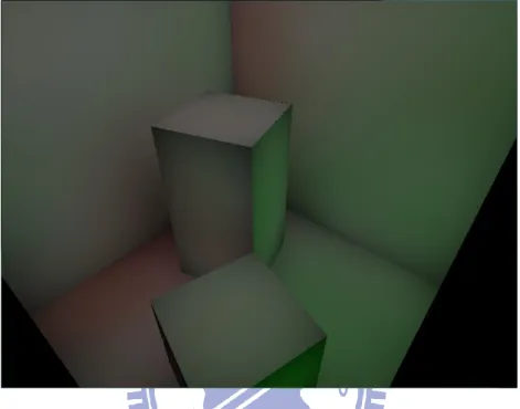
the image after hardware alpha blending is the indirect radiance. We can add it in soft shadow pass directly without combining direct lighting result and indirect lighting result separately. In fact we combine indirect light, soft shadow and up-sampling pass into one pass. After

adjusting splatting radius the indirect lighting result will like Figure 3.9.

Figure 3.9 Splatting result without blending with soft shadow

3.4 Image Space Soft Shadow

Our algorithm generates soft shadow during deffered shading step. As mention before, we chose image space soft shadow algorithm instead of ambient occlusion or other soft shadow method. Since our work is to combine two algorithm, the more pass they are analogous, the more information they can share. This reduce the total computation of the algorithm. Sowe follw the method [17] which uses bilateral filter to blur shadow edges with 3D geometry information stored in G-buffer. Image space gathering shadow has two steps. First, find the average distance to occluders of each pixel rendered by deffered shading. Second, with the average distance to occluders, we can blur each shading pixel with individual shadow penumbra radius.

15

R_p = L Z_eye (2)

Where L is a scaling factor representing the size of virtual area light and Zeye is the eye space

depth value used to project the light radius into screen space.

Figure 3.10 Image space gathering

The goal of the first step is to find the weighted average distance to occluders. We filter those distances by the flowing equation：

g(p ₀) = Ni =0ω(p i,p 0)γ(p i,p 0)𝐼(p i) ω(p i,p 0)γ(p i,p 0) N

i=0

(3)

Where I is the image data, N is the number of pixels in shadow, p _i is the pixel in search range, ω(p i, p 0) is a constant weighting function and γ(p i, p 0) is the range function which

is：

γ(p i, p 0) = e−ι 2_/σ

(4)

Where

ι

is the world space distance of p i and p 0.

Second, with the weighted average distance, d, to occluder, we then compute the blur region radius Rg which is：

R_g = L d

D−d∙

1

16

where D is the space distance from the shaded point to the light. Next we search with radius

Rg and use the filter function as Equation (3). Then we get the blur shadow image as shown in

Figure 3.11 (b).

Figure 3.11 The result (a) without and (b) with soft shadow

3.5 Image Space Radiance Interpolation

After we compute indirect and direct illumination with soft shadow, we continue to combine them together. Although we have simplified the photon volume as photon quad and use Optix to trace photon on GPU, the indirect lighting computation is still expensive. In order to improve the performance of indirect lighting computation, we can optionally down-sample radiance from the photons and then use geometry-aware filtering to up-sample the resulting screen space radiance to estimate the final image resolution.

The idea is to compute indirect lighting only at fewer locations in screen space , which produce a low resolution indirect light radiance map. Next, for remaining pixels, we use interpolation to obtain their color by comparing full resolution normal map and depth map. That is, for each pixel rendered at the final step, we search the nearby four sub-pixels the same as bilinear interpolation. Simultaneously, we comparing these sub-pixels with the rendering pixel by their normal and depth. Therefore, we can choose sub-pixels which are on

17

the same plane of rendered pixel or nearby sub- pixels in a certain space distance to interpolate while preserves object edges and corners.

Figure 3.12 (a) 8x8 Subsampling. (b) Bilinear weighting

In detail, first, we render indirect lighting by 8x8 sampling with nearest-neighbor upsamples, as shown in Figure 3.12 (a). Then we apply bilinear interpolation with only screen space distance weighting, as shown in Figure 3.12 (b). In order to preserve corners and edges, it is further weighted by the dot product of normal and difference of depth, as shown in Figire 3.13. Compare to the 1x1 sampling image, as shown is Figure 3.14, we dramatically enhance the performance by losing a little quality.

18

Figure 3.13 Result after normal and depth weighting

19

Chapter 4

Implementation Detail

Since our approach bases on photon mapping, we can handle most optical phenomena such as indirect lighting and caustic with physical accuracy. However, photon mapping have two major risk, path tracing and computation of photon radiance contribution. Path tracing is highly dependent on the scene, the cost increases with the complexity of scene. Fortunately, with the GPU-based ray tracing engine, we can handle this by optimized multi-processing. Moreover, by taking the advantage of GPU rasterization path, we abstain the final gathering.

We implement our approach by using OpenGL with CgFX shader language, and implement photon tracing with Optix [13]. In our approach, any geometry data should be sent into both Optix host and OpenGL. We use OpenGL Vertex Array Object(VAO) to share geometry data with Optix and OpenGL. Since we use VAO, both Optix and OpenGL can access the geometry data directly in GPU memory without copy memory into the main memory. Furthermore, VAO not only can take geometry data to be reused but can avoid copy photon map from GPU to CPU memory. After Optix finishs photon tracing and outputs a photon map, we can use VAO to copy photon data as OpenGL primitive input. Note that the memory bus between CPU main memory and GPU memory which is called Peripheral Component Interconnect Express(PCI-Express) bus has only max 8 GB/s data rate. It is very slow transmission speed comparing to other data bus in computer. If we copy buffer between GPU and CPU memory frequently , it is bound to reduce performance acutely. By using OpenGL Frame Buffer Object, we can access buffer data in GPU memory immediately after the previous rendering pass.

20

When sending mesh data into Optix, we must construct geometry group in Optix context. The geometry structure in Optix is shown in Figure. A geometry group can contain many geometry instances. For each geometry instance, it has primitive data with intersection program and material program. We bound primitive data by bounding program, and the Optix will generate BVH to accelerate the computation of intersection. The intersect program define the way how we find the intersection position on mesh surface. So we can use multiple kind if structure to describe model surface such as triangle, parallelogram or sphere...etc. Once the intersect program return an intersection event, we can obtain the texture coordinate, normal and color data of the hitting point. However, for external material information such as shadow or indirect light which cannot obtain by intersect program. We can obtain these external material from any-hit or closet-hit program by continue tracing rays from hitting position. In our implementation we trace shadow rays in any-hit program and photon path ray in closet-hit program. Note that the different between any-hit and closet-hit is using the ray payload or not. Any-hit program can only return hit object or not. While closet-hit can obtain color, normal and distance of intersection point by storing these data into ray payload.

Figure 4.1 Optix data structure

Geometry Group

Geometry Instance

Geometry Intersect and bounding

Material

21

Chapter 5

Results and Discussion

In this section, we present our results rendering at real-time frame rates on a desktop PC with Intel Core i7 930 CPU 2.8GHz and NVIDIA GeForce GTX 480 video card.

All results are rendered at 1024 x 768 pixels.

Figure 5.1 ~ 5.4 show scenes rendered by our algorithm. Figure 5.1 and Figure 5.2 display basic Cornell box scene illuminated by once and twice bounce indirect lighting with soft shadow effect. Figure 5.3 and Figure 5.4 demonstrate Cornell box containing a complex model with diffuse material. Figure 5.5 and Figure 5.6 show glass object (η = 1.5 with a little reflect and fresnel effect). Eye-ray refraction is computed for front faces using dynamic environment map with direct light only. The image also demonstrates refractive caustic phenomena. Figure 5.7 and Figure 5.8 show the complex scene of Sponza and Sibenik.

22

Figure 5.2 Happy buddha

23

Figure 5.4 Glass sphere

24

Figure 5.6 Sibenik

25

Since we use 2D photon quad instead of photon volume. We avoid the artifacts arised by the clipping of photon volume when the camera close to a surface. We also speed up the GPU radiance estimation procedure. However, because we splat photon on surface plane, the contribution of photons at corner will be clipped by normal weighting. Specific regions such as refractive caustic will discontinue while across the corner. But this artifact can be eliminated by increasing the number of photons.

Table 1 shows the experimental results of our rendering algorithm. We can find out that the soft shadow generation is very time-consumed. Since we can speed up by reducing the sampling number of image space gathering, user can trade rendering quality for speed. Moreover we can also abandon the average distance to occluders and just apply blur in a certain radius alone the shadow edge. Note that the Sponza Atrium scene with larger photon radius cause lower frame rate and higher quality.

Scene Polygons Sub- sampling Bounce Photons (radius) Samples fps(hard) Cornell box 30 8x8 1 10k(4.5) 4+5 32(107) Cornell box 30 8x8 2 20k(4.5) 4+5 27(85) Happy buddha 50,020 4x4 1 10k(4.5) 4+5 20(40) Chinese dragon 26,082 4x4 3 30k(4.5) 4+5 23(35) Glass sphere 9,220 4x4 2 20k(4.5) 4+5 34(70) Glass bunny 32,134 4x4 2 20k(4.5) 4+5 32(63) Sibenik 80,054 2x2 2 20k(8.5) 4+7 12(35) Sponza Atrium 67,461 2x2 2 20k(10.5) 4+7 9(20) Table 1：Detail performance statistics for scenes. The "hard" behind fps means fps of hard shadow result. The "radius" is the photon splat size.

26

We also compare the rasterization speed of the original ISPM method. Table 2. shows the compare result, note that the icosahedron in our implement is uncompressed so the icosahedron photon can influence more region and make result more bright . We use geometry shader to output 20 triangle to form an icosahedron. Then we use the similar photon scattering computation. We falloff the photon energy by the distance of shaded pixel position and the photon center, and use equation(1) in Section 3.3 to compute the radiance. In our experiment the raster time increase with the number of photons, when the photon number increase than thirty thousand, our method can speed up to 10fps than the original method.

Figure 5.8 and figure 5.9 show the different result of using icosahedron and quad. Since we use quad to bound photon and can affect plane with similar normal. Region in object corner will have less photon contribution. This can explain as the effect of ambient occlusion. Users can alternative use icosahedron in those corner area to remove such ambient occlusion effect. Scene Sub- sampling Bounce Photons (radius) fps(hard) Quad fps(hard) Icosahedron Cornell box 8x8 2 20k(4.5) 22.0(61.0) 21.0(60.7) Cornell box 8x8 3 30k(4.5) 23.0(61.4) 20.4(54.0) Happy buddha 8x8 3 30k(4.5) 11.7(42.1) 11.3(37.2) Chinese dragon 8x8 3 30k(4.5) 21.2(56.3) 20.5(50.9) Glass bunny 8x8 3 30k(4.5) 22.0(60.3) 20.6(51.4) Sibenik 8x8 3 30k(8.5) 22.0(43.0) 18.9(33.0) Sponza Atrium 8x8 3 30k(8.5) 27.5(46.4) 24.7(39.5) Table2：Compare performance for scenes. We use the same sample rate of the soft shadow(4+5), and the same sub-sampling rate(8x8).

27

28

29

Chapter 6

Conclusion And Future Work

In this thesis, we propose a GPU-based real-time global illumination algorithm that extend image-space photon mapping with soft shadow effect. We simplify the photon splatting phase of ISPM[12] and reduce the total pass number. Our algorithm implement entirely on GPU and avoid coping memory data between CPU and GPU. We preserve the benefit of two algorithm, so we can also handle multiple bounce of indirect lighting and complex optical phenomena such as caustic in real-time speed.

However, as mentioned before, the image space soft shadow still takes too much time. Since it has to blur each pixel to generate soft shadow edge, the computation cost increases with the resolution of the final image and the number of pixels in shadow region. Although we can reduce the sampling number, in order to get compelling approximations of soft shadows, we should keep a certain number of samples. One of our future work is to speed up the generation of soft shadow.

In the future we also like to extent our method to handle translucent objects. Since we use ray tracing to trace the photon, we can use subsurface scattering method to compute reflected direction after multiple scattering when ray hit translucent objects. And then use pre-computed scattering texture to compute the radiance of each pixel when photons splat on translucent objects.

30

References

[1] APPEL, A. 1968. Some techniques for shading machine renderings of solids. In AFIPS ’68 (Spring): Proceedings of the April 30–May 2, 1968, spring joint computer conference, ACM, New York, NY, USA, 37–45.

[2] COOK, R. L., PORTER, T., AND CARPENTER, L. 1984. Distributed ray tracing. In Proceedings of SIGGRAPH, 137–145.

[3] DACHSBACHER, C., AND STAMMINGER, M. 2005. Reflective shadow maps. In Proc. of ACM SI3D ’05, ACM, New York, NY, USA, 203–231.

[4] FERNANDO, R. 2005. Percentage-closer soft shadows. In SIGGRAPH Sketch.

[5] HERZOG, R., HAVRAN, V., KINUWAKI, S., MYSZKOWSKI, K., AND SEIDEL, H.-P. 2007. Global illumination using photon ray splatting. In Eurographics 2007, vol. 26, 503–513.

[6] JENSEN, H. W. 1996. Global illumination using photon maps. In Proceedings of the eurographics workshop on Rendering techniques’96, Springer-Verlag, London, UK, 21–30.

[7] KELLER, A. 1997. Instant radiosity. In SIGGRAPH ’97: Proc. of the 24th annual conference on comp. graph. and interactive techniques, ACM Press/Addison-Wesley Publishing Co., New York, NY, USA, 49–56.

[8] LAINE, S., AND KARRAS, T. 2010. Two Methods for fast ray-cast ambient occlusion. In Proceedings of Eurographics Symposium on Rendering 2010.

[9] LANDIS H. 2002. Production-ready global illumination. Course notes for SIGGRAPH 2002 Course 16, RenderMan in Production.

31

hashing. In HWWS ’02: Proc. of the ACM SIGGRAPH/EUROGRAPHICS conf. on Graph. hardware, Eurographics Association, Aire-la-Ville, Switzerland, 89–99.

[11] MCGUIRE, M. 2010. Ambient occlusion volumes. In Proceedings of the 2010 ACM SIGGRAPH/EuroGraphics conference on High Performance Graphics.

[12] MCGUIRE, M., AND LUEBKE, D. 2009. Hardware-Accelerated Global Illumination by Image Space Photon Mapping. In Proceedings of the 2009 ACM SIGGRAPH/EuroGraphics conference on High Performance Graphics.

[13] PARKER, S. G., BIGLER, J., DIETRICH, A., FRIEDRICH, H., HOBEROC, K J., LUEBKE, D., MCALLISTER, D., MCGUIRE M., MORLEY, K., ROBISON, A., STICH, M. 2010. Optix: A general purpose ray tracing engine. ACM Transactions on Graphics.

[14] PURCELL, T. J., DONNER, C., CAMMARANO, M., JENSEN, H. W., AND HANRAHAN, P. 2003. Photon mapping on programmable graphics hardware. In Proceedings of the ACM SIGGRAPH/EUROGRAPHICS Conference on Graphics Hardware, Eurographics Association, 41–50.

[15] RITSCHEL, T., ENGELHARDT, T., GROSCH, T., SEIDEL, H.-P., KAUTZ, J., AND DACHSBACHER, C. 2009. Micro-rendering for scalable, parallel final gathering. ACM Trans. Graph. 28, 5, 1–8.

[16] RITSCHEL, T., GROSCH, T., KIM, M., SEIDEL, H.-P., DACHSBACHER, C., AND KAUTZ, J. 2008. Imperfect shadow maps for efficient computation of indirect illumination. ACM Trans. Graph. 27, 5, 1–8.

[17] ROBISON, A., AND SHIRLEY, P. 2009. Image space gathering. In Proceedings of the 2009 ACM SIGGRAPH/EuroGraphics conference on High Performance Graphics. [18] SAITO, T., AND TAKAHASHI, T. 1990. Comprehensible rendering of 3-d shapes.

SIGGRAPH Comput. Graph. 24, 4, 197–206.

32

gpu-based approach for interactive global illumination. ACM Trans. Graph. 28, 3, 1–8. [20] ZHUKOV S., IONES A., KRONIN G. 1998. An ambient light illumination model. In

Rendering Techniques 98 (Proceedings of Eurographics Workshop on Rendering), pp. 45–55.