ALGORITHMS FOR THE RURAL POSTMAN PROBLEM

(1)

Pergamon _{o3os-o~s(94)oooTo-o}

A L G O R I T H M S F O R T H E R U R A L P O S T M A N P R O B L E M

W. L. P e a r n t t and T. C. Wu2+ +

Department of Industrial Engineering & Management, National Chiao Tung University, 1001 Ta Hsueh Road, Hsinchu, Taiwan 30050, R.O.C. and 2Tsuyung Senior Commercial and Industrial

Vocational School, Taichung, Taiwan, R.O.C.

(Received March 1994; in revised form September 1994)

Scope and Purpose--Given an undirected (connected) street network, the well-known Chinese postman problem (CPP) is that of finding a shortest (or least-cost) postman tour covering all the edges (streets) in the network. The rural postman problem (RPP), is a generalization of the CPP, in which the underlying street network may not form a connected graph. Such situation occurs, particularly, in rural (or suburban) areas where only a subset of the streets need to be serviced. The RPP has been shown to be NP-complete, and heuristic solution procedures have been proposed to solve the problem approximately. The purpose of this paper is to review the existing solution procedures, and introduce two new algorithms to solve the problem near-optimally.

Abstract--The rural postman problem (RPP) is a practical extension of the well-known Chinese postman problem (CPP), in which a subset of the edges (streets) from the road network are required to be traversed at a minimal cost. The RPP is NP-complete if this subset does not form a weakly connected network. Therefore, it is unlikely that polynomial-time bounded algorithms exist for the problem. In this paper, we review the existing heuristic solution procedures, then present two new algorithms to solve the problem near-optimally. Computational results showed that the proposed new algorithms significantly outperformed the existing solution procedures.

1. INTRODUCTION

Given a connected undirected network G=(V, E) with a set of nodes V and a set of edges E, then the celebrated Chinese postman problem (CPP) is that of finding a shortest (or minimal-cost) postman tour such that each edge in E is traversed at least once. The rural postman problem (RPP) is a practical extension of the CPP, in which only a subset of the edges in E are required to be traversed at minimal cost. Such an extension, of course, accommodates real-world situations more closely. In particular, for rural (or suburban) areas where only a subset of the streets need to be serviced.

The R P P was first introduced by Orloff [1], and has received some research attention recently [2-4]. The R P P can be briefly defined as follows. We are given an undirected graph G=(V, E, ER) with V representing the set of nodes, E representing the set of edges (streets), and ER (~_E) representing the set of edges that must be serviced. Then, the R P P is to find a postman tour, starting from the depot, traversing each edge in E R at least once, and returning to the same depot with total distance (cost) minimized. Clearly, if Ea = E, then the R P P reduces to the CPP.

Real-world applications directly related to the R P P include: routing of newspaper or mail delivery vehicles, parking meter coin collection or household refuse collection vehicles [7], street sweepers, snow plows and school buses [8]; spraying roads with salt [9, 10], inspection of electric power lines, or oil or gas pipelines, and reading electric meters [11].

-t'W. L. Pearn received his Ph.D. degree from University of Maryland at College Park, Maryland. His areas of interest include network optimization, and quality management. He has been with AT&T Bell Laboratories, and currently he is a professor of Operations Research in the Department of Industrial Engineering and Management at National Chiao Tung University, Taiwan, R.O.C.

++T. C. Wu received his M.S. degree from Department of Industrial Engineering and Management, National Chiao Tung University. Currently, he is an instructor of Tsuyung Senior Commercial and Industrial Vocational School.

(2)

The RPP has been shown to be NP-complete if the required set of edges, E a, does not form a weakly connected network but forms a number of disconnected components. Christofides et al. [2] presented an integer programming formulation of the problem, and developed an exact algorithm to solve the RPP optimally. The algorithm is essentially based on a branch-and-bound algorithm using Lagrangean relaxations. Unfortunately, their approach requires an exponential algorithm and is computationally inefficient; only problems of small and moderate size can be solved within reasonable amount of computer time. Because of the problem's complexity, a heuristic solution procedure [21 has been proposed to solve the problem approximately. In this paper, we first review this heuristic solution procedure, then present two new algorithms to solve the problem near-optimally.

2. EXISTING SOLUTION PROCEDURES

Christofides et al. [2] presented a heuristic solution procedure to solve the RPP approximately. The algorithm essentially consists of three phases. Phase I transforms the subnetwork (GR) containing the required edges (ER) into a complete network. Phase II applies the minimal spanning tree algorithm to render GR connected. Phase III applies the minimal-cost matching algorithm to obtain an Eulerian network. The postman tour then can be constructed from the resulting Eulerian network. In the following, we briefly review this heuristic solution procedure.

(A) Christofides et al. A l g o r i t h m

Phase I (Graph transformation)

Step 1. Let G R = ( V R , ER) be the subnetwork consisting of the required edges, E~, and the corresponding set of nodes, V R. Transform GR into a complete network by adding an edge between every pair of nodes in GR. Let E A be the set of artificial edges generated from this transformation. The cost of an edge (i, j) in E A is defined as cij=the shortest path length between the nodes i and j from the original network. Call the resulting network Ggco = (VR, ER u EA). Step 2. Simplify Gsc,, by eliminating: (1) all edges (i, j)6 E A for which the edge cost

cij = Cik + Ck~ for some k, and (2) one of the two edges in parallel if they both have the same cost. Call the resulting network GRc.

Phase II (Minimal spanning tree)

Step 1. Let {C1, Ca . . . Cr} be the set of components from GR, and G c the condensed graph obtained from G R by treating each component as a node. An edge (i, j) of Gc exists if there exists an edge (x, y) 6 GRc with x 6 C~, y ~ Ci. Define the cost of an edge (i, j)6 G c as d(i, j ) = d(Ci, C ) = minx.r{d(x, y ) - u x - uy}, where ux, ur are multipliers.

Step 2. Apply the minimal spanning tree (MST) algorithm over G o Let E T be the set of edges from the MST solution.

Phase Ill (Minimal-cost matching)

Solve the CPP over GR ~ ET by applying the minimal-cost matching algorithm [12-1 to obtain an Eulerian network. Let E M be the set of edges from the matching solution. Then, the resulting network GR u E T ~ E M, is the desired RPP solution.

For the multipliers, Ux and yy, Christofides et al. [2] considered u i = -r/(deg(i)-2), where deg(i) is the degree of node i from the original network G. This algorithm requires the application of the minimal-cost matching algorithm, which is of O(IVI3), where [VI =the number of nodes from the original network G. Therefore, the complexity of Christofides et al. algorithm is 0([ V 13). In the case where the underlying network satisfying the triangular inequality property, Benavent et al. [4] showed that the performance of this algorithm, in the worst case, has a bound of 3/2. That is (Christofides et al. Solution)/(Optimal Solution)~< 3/2. In the following example, we show that this bound is reachable.

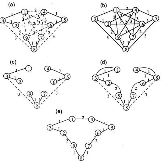
E x a m p l e I. Consider the RPP network depicted in Fig. l(a) with nine nodes forming three components, {(1, 3), (2, 3)}, {(4, 5), (5, 6)}, and {(7, 8), (8, 9)}. Christofides et al.'s algorithm first performed the transformation (Phase I) converting the original network into one (GRc) shown in

(3)

Algorithms for the rural postman problem 821

(a)

~ = , ~ ' , , zt.&r -!- ,, , " " , ~ , ~,',3x"x~," 2 , "

(b)

3

(c)

J N j

3",@ @,,'3

(el

(d)

, f 1 2 2 Fig. I. (a) T h e o r i g i n a l R P P n e t w o r k in E x a m p l e 1. (b) T h e t r a n s f o r m e d n e t w o r k . (c) T h e r e s u l t i n g n e t w o r k a f t e r a p p l y i n g t h e M S T a l g o r i t h m . (d) T h e r e s u l t i n g n e t w o r k after a p p l y i n g the m a t c h i n g a l g o r i t h m . (e) T h e o p t i m a l R P P s o l u t i o n .

Table 1. Parameter analysis of Christofides et al. algorithm (10 problems). Underlines indicate the best solution) Problem

number IVI I V~;=l I EI I ERI q = 1 t/= 2 q = 3 q = 4 r/= 5 q = 6

1 29 3 79 43 510 510 526 526 526 526 2 43 4 203 42 471 475 475 475 482 482 3 25 5 84 24 320 328 327 341 341 341 4 37 6 79 38 421 421 425 425 425 435 5 33 7 99 33 359 359 372 371 371 385 6 25 8 75 16 284 301 301 301 295 295 7 39 9 85 31 418 415 439 439 449 449 8 46 10 199 37 501 500 516 516 516 516 9 49 II 140 35 433 445 447 466 466 466 10 43 12 117 32 406 422 428 427 431 431

Fig. l(b). The algorithm then proceeded with applying the minimal spanning tree algorithm (Phase II) generating artificial edges Er = {(3, 8), (5, 8)}. The resulting network is displayed in Fig. l(c). The Christofides et al. algorithm terminated with applying the minimal-cost matching algorithm (Phase III), generating artificial edges EM = {(1, 3), (4, 5), (2, 9), (6, 7)}. The resulting network, shown in Fig. l(d), constitutes an R P P solution with a total cost of 18. We note that the same solution can be obtained for any chosen multiplier r/, r/>0. Since the optimal solution for this problem (see Fig.

le), has a total cost of 12, we have (Christofides et al. Solution)/(Optimal Solution)=3/2.

We experimented with the Christofides et al. algorithm on l0 sample problems, where q was initially set to q = l, 2, 3, 4, and 5. The results, displayed in Table l, indicated that the solution obtained on these problems achieved best problem solutions for r/= l and 2, and that the solution

(4)

values increased for other q values. Therefore, we limited the choice of multipliers for this algorithm t o q = l and 2.

3. NEW ALGORITHMS

We point out that the performance of the Christofides et al. algorithm can be greatly affected by the values of the chosen multipliers, r/. In addition, we feel that Phase I of the algorithm (graph transformation) contributed insignificantly in obtaining efficient solutions although the transformation simplifies the problem structure in formulating the RPP. In attempting to improve the solution, we propose the following modifications. The modified approach considers the new distance d(C~, C j) = minx.y{spl(x, Y) I x ~ C~, y ~ Cj} + 2 with a penalty 2 (rather than d(C;, C j) =minx,r{d(x, y ) - u ~ - u y } ) added in defining the distances in the condensed network Go where spl(x, y) is the length of the shortest path between node x and node y from the original graph G. Obviously, different penalty values generate different R P P solutions. Therefore, we can choose a set of 2 values to generate some R P P solutions, then select the best among all as the solution from this approach. The modified approach can be described as follows.

(B) Modified Christofides et al. AIoorithm Phase I (Minimal spanning tree)

Step 1. Define the distance between every pair of nodes i, j e Gc as d(i, j) = d(C~, C~) = minx,y{spl(x, y)lxeC~, y~ C j} +2, with 2 set to 2 o = 0 initially. Apply the minimal spanning tree (MST) algorithm over Go Let Er0(2) be the set of edges from the minimal spanning tree solution.

Step 2. Simplify Er0(2) by eliminating all the duplicated copies of the edges that are in parallel. Call the resulting set of edges Er(2).

Phase II (Minimal-cost matching)

Solve the C P P over GREET(2) by applying the minimal-cost matching algorithm [-12] to obtain an Eulerian network. A postman tour then can be constructed from this Eulerian network. Let EM(2) be the set of edges from the matching solution. Call the resulting R P P solution G(2) = GR u ET() 0 ~ EM(2).

Phase III (Iterations with varied parameter values)

Repeat Phases I and II for a set of chosen values {21, 22 . . . 2k} for the penalty parameter 2, generating a set of R P P solutions {G(2~)}, i=0, 1, 2 . . . k. Select the best (with the smallest value) among all as the solution from this approach.

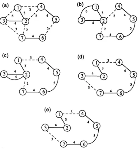
Example 2. Consider the R P P network depicted in Fig. 2(a) with seven nodes forming three components, {(1, 2), (2, 3)}, {(4, 5)}, and {(6, 7)}. It is straightforward to verify that the modified approach obtains solutions with values equaling 30, 29, 26, 26 for 2 =0, 1, 2, and 3, respectively (see Fig. 2b, c, d, and e). Therefore, the solution for the modified approach is 26, which is optimal.

We note that for the R P P described in Example 1, the Christofides et al. algorithm obtained a solution with a value (18) that is 1.5 times that (12) of the problem optimal solution. But, if we apply the modified approach with the penalty parameter )4 set to 2 = 0, then the optimal solution, which has a value of 12, can be obtained.

It should be noted that in applying the minimal spanning tree algorithm to connect the components in G o the penalty parameter, 2, is added to the distance d(i, j) = d(C i, C i) only for those (i, j) in Ex(2o). We experimented with the algorithm on the same 10 test problems described previously using seven values of 2, which were initially set to 2 = 0, 1, 2, 3, 4, 5, and 6. The results are displayed in Table 2. It appeared that the solution obtained on these problems achieved best problem solutions for 2 = 0, 1,2, and 3, and that solution values increased when 2 exceeded the range of [0, 3]. Therefore, we limited the choice of penalty values for this algorithm to 2 = 0, 1, 2, and 3.

(C) Reverse Christofides et al. Algorithm

The approaches by reversing the steps (or phases) of the existing solution procedures have been considered in developing new solution strategies [13-15]. In some cases, the reverse approaches

(5)

Algorithms for the rural postman problem 823

(a)

"- "

3 /5

5 /

~2

5/

3 4

(d)

- 4

@,

Fig. 2. (a) The original R P P network in Example 2. (b) The modified approach solution for ,;.=0. (c) The

modified approach solution for ,;. = I. (d) The modified approach solution for 2 = 2. (e) The modified approach solution for 2 = 3.

Table 2. Parameter analysis of the modified Christofides et al. algorithm (10 problems}. (Underlines indicate the best solution) Problem

number JVt IVG¢I IEI IERI 2 = 0 2 = 1 ,;.=2 2 = 3 ),=4 , . = 5 ).=6

1 29 3 79 42 510 510 508 508 510 510 510 2 43 4 203 42 46___~7 46"/ 46"/ 471 471 471 471 3 25 5 84 24 319 319 31____55 319 319 319 319 4 37 6 79 38 419 41__Jl 41__..11 411 417 419 419 5 33 7 99 33 349 345 345 345 349 349 349 6 25 8 75 16 294 293 28__..44 292 294 294 294 7 39 9 85 31 437 407 409 409 409 409 409 8 46 10 199 37 501 496 498 501 501 501 501 9 49 11 140 35 430 430 429 421 420 430 430 10 43 12 117 32 404 402 404 404 404 404 404

perform remarkably well. Recall that the Christofides et al. algorithm consists of two main segments, the minimal spanning tree and the minimal-cost matching. The reverse approach of the Christofides

et al. algorithm, in this case, first applies the minimal-cost matching, then the minimal spanning tree

algorithms.

Phase I (Minimal-cost matching)

Define the distance between every pair of nodes i, j e GR as d(i, j) = minx.r{spl(x, y)] + )., with 2 set to 2 o = 0 initially, where spl(x, y) is the length of the shortest path between node x and node y from the original graph G. Apply the minimal-cost matching algorithm [12] over G~. Let EM(2) be the set of edges from the matching solution.

(6)

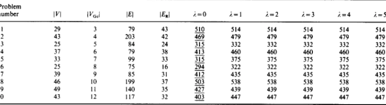
Table 3. Parameter analysis of the r e v e r s e Christofides e t al. algorithm (10 problems}. (Underlines indicate the best solution} Problem

number IVI IV~°I IEI IEkl 2 = 0 2 = 1 , . = 2 ,;.=3 ,;.=4 ,;.=5

I 29 3 79 43 510 514 514 514 514 514 2 43 4 203 42 469 479 479 479 479 479 3 25 5 84 24 315 332 332 332 332 332 4 37 6 79 38 413 460 460 460 460 460 5 33 7 99 33 315 375 375 375 375 375 6 25 8 75 16 294 322 322 322 322 322 7 39 9 85 31 412 435 435 435 435 435 8 46 10 199 37 503 538 538 538 538 538 9 49 11 140 35 427 439 439 439 439 439 10 43 12 117 32 403 447 447 447 447 447

Phase II (Minimal spanning tree).

Step 1. Apply the minimal spanning tree algorithm over the condensed network obtained from GK w Eu(2) by treating each component as a single point. Let Ero(2) be the set of edges from the minimal spanning tree solution.

Step 2. Remove all duplicated edges from Exo(2), and let ET(2) be the resulting set of edges (after removing duplicated edges). Then, GRWEM(2)WET().)WET(2 ) is the desired RPP solution.

Phase III (Iterations with varied parameter values).

Repeat Phases I and II for a set of chosen values {2~, 22 . . . 2k} for the penalty parameter 2, generating a set of RPP solutions {G(2i) }, i=0, 1, 2 . . . k. Select the best (with the smallest value) among all as the solution from this approach.

We note that in applying the minimal-cost matching algorithm (Phase I) to obtain an even network, the penalty parameter, 2, is added to the distance d(i, j) only for those (i, j) in EM(2o). The penalty values, 2, for the reverse approach are automatically set to 2 = 0, 1, 2, and 3 initially (same as that for the original algorithm). The results of our preliminary experiments (see Table 3) indicated that the reverse approach achieved best problem solutions (10 out of 10 problems) for 2=0. We therefore set the choice of parameter values of the reverse approach to ,~. = 0.

4. C O M P U T A T I O N A L C O M P A R I S O N S

For the purpose of testing the proposed new solution procedures (modified and reverse approaches) and comparing them with the Christofides et al. algorithm, we generate 10 sets, a total of 200 problems. These problems are generated by randomly linking a pair of nodes, forming networks with various numbers of components. Their sizes range from three components, 15 nodes, 31 edges with 11 required edges, to 12 components, 52 nodes, 266 edges with 61 required edges. The edge lengths of these problems are also randomly generated, ranging from 1 to 20. These test problems are described in the following with I VI representing the number of nodes from the original

network, IVG¢I representing the number of components, IEI representing the number of edges, and IEal representing the number of required edges.

Set A: 20 problems; I Vc¢l = 3, 15 ~< I VI ~< 40, 11 ~< IERf ~< 47, 31 ~< IEI ~< 157; Set B: 20 problems; IV6c1=4, 24~<1V1~<42, 25~<1E~1~<49, 40~<1E1~<203; Set C: 20 problems; IVGcI=5, 24~<1V1~<43, 19~<1ER1~<48, 68~<1E1~< 189; Set D: 20 problems; IVG¢I=6, 22~<1V1~<45, 18~<1ER1~<46, 46~<1E1~< 170; Set E: 20 problems; IV~¢1=7, 21 ~lVl~50, 15~<IERI~<61, 51 ~<IEI~< 119; Set F: 20 problems; IVcd=8, 25~<1V1~<49, 16~<1ER1~<49, 59~<1Er~<178; Set G: 20 problems; IVG¢I=9, 26~<1V1~<49, 16~<1Ea1~<47, 51~<1Et~<266; Set H: 20 problems; IVocl = 10, 31 ~<1V1~<47, 17~<1ER1~<44, 60~<1E1~<211; Set I: 20 problems; IVGJ = 11, 29~<1V1~<52, 16~<1E~1~<38, 48~<1E1~< 148; Set J: 20 problems; IV~¢I=12, 29~<1V1~<48, 17~<IEa}~<41, 63~<1E}~<211.

(7)

Algorithms for the rural postman problem Table 4. Number of problems receiving the best solution

825

Problem Number of Christofides Modified Reverse

set problems II/I IEI IERI algorithm Cbristofides Christofides

A 20 15-40 31-157 11--47 6 19 10 B 20 24-43 40-203 25-49 2 13 l0 C 20 24-43 68-189 19-48 2 11 13 D 20 22-45 46-170 18-46 2 12 9 E 20 21-50 51-199 15-61 2 12 8 F 20 25-49 59-178 16-49 2 12 1 I G 20 2 6 ~ 9 51-266 16-47 1 11 11 H 20 31 47 60-211 17-44 1 16 6 1 20 29-52 48-148 16-38 I 13 6 J 20 29 48 63 211 17~.1 2 14 6

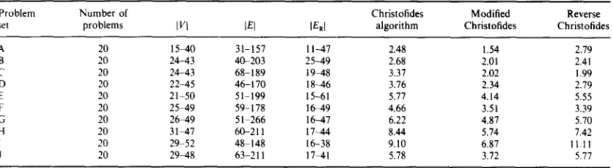
Table 5. Average percentage above the problem's lower bound

Problem Number of Christofides Modified Reverse

set problems I VI LEI IERI algorithm Christofides Christofides

A 20 15 40 31-157 11-47 2.48 1.54 2.79 B 20 24-43 40-203 25-49 2.68 2.01 2.41 C 20 24-43 68-189 19-48 3.37 2.02 1.99 D 20 22-45 46-170 18-46 3.76 2.34 2.79 E 20 21-50 51-199 15-61 5.77 4.14 5.55 F 20 25-49 59-178 16-49 4.66 3.51 3.39 G 20 26-49 51 266 16-47 6.22 4.87 5.70 H 20 31 47 60-211 17-44 8.44 5.74 7.42 I 20 29-52 48-148 16-38 9.10 6.87 I 1.11 J 20 29-48 63-211 17-41 5.78 3.72 5.77

Table 6. The ~orst solution in terms of percentage above the lower bound

Problem Number of Christofides Modified Reverse

set problems bt" I IEh IERI algorithm Christofides Christofides

A 213 15 40 31 157 11-47 14.38 10.18 14.52 B 20 24 43 40-203 25-49 7.74 7.78 11.27 ( 20 24 43 68 189 19 48 6.87 5.68 6.44 D 20 22 45 46 170 18- 46 10. l I 7.87 6.9 I E 21) 21 50 51-199 15-61 21.05 17.37 34.55 F 20 25-49 59 178 16-49 8.05 9.04 12.08 (; 21~ 26-49 51 266 16-47 15.79 15.33 21.33 !t 20 31 47 60-21 I 17-44 30.38 22.69 37.69 I 20 29 52 48.-148 16-38 22.01 20.71 51.18 J 20 29-48 63 211 17-41 13.64 14.94 27.27

We ran through these 10 sets, 200 test problems for the three algorithms original, modified, and the reverse approaches. We compared their performance with respect to (1) number of problems receiving the best solution, (2) the average percentage above the problem lower bound, and (3) the worst solution in terms of percentage above the problem lower bound. The results on the 10 sets of test problems are displayed in Tables 4, 5, and 6. Table 7 summarizes the performance comparisons of the three algorithms on the 200 test problems, including (4) average rank among the three algorithms, and (5) the number of problems achieving the problem lower bound (hence the solution must be optimal). We note that the lower bounds, used as a convenient reference point for assessing the accuracy of the heuristic solutions, were obtained from solving the CPP over the subnetwork GR. In comparing the modified and the original approaches, the test results showed that:

(1) The modified approach improved the original algorithm (excluding ties) for 14, 16, 16, 17, 16, 16, 16, 19, 18, 17 problems (out of 20) respectively in the 10 sets of test problems (an average of 82.5%);

(2) The modified approach improved the original algorithm for 1.55% (on the average) in terms of percentage above the problem lower bound;

(3) The modified approach received 133 best solutions (including at least 11 optimal solutions) out of 200 test problems (an average of 66.5%). Compare this with 21 best solutions (including

(8)

Table 7. Performance comparisons of the three algorithms 1200 problems}

Christofides Modilied Reverse algorithm Christolides Christofides

Average % above the lower bound 5.23 3.68 4.89

Average rank among the three algorithms 2.43 1.38 1.74 N umber of problems receiving the best solutions 21 133 90 Worst solution among 200 problems in terms

of % above the lower bound 30.38 22.69 51.18

Number of problems achieving the lower bound 2 11 6

Table 8. Run time comparisons lin C P U secondsl of the three algorithms

Problem Number of Christofides Modified Reverse

set problems I VI IEI levi algorithm Christofides Christofides

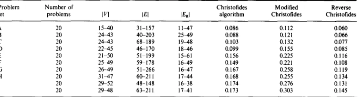
A 20 15-40 31-157 11-47 0.086 0.112 0.060 B 20 24-43 40-203 25-49 0.088 0.121 0.066 C 20 24-43 68-189 19~.8 0.103 0.132 0.077 D 20 22~45 46-170 18~.6 0.099 0.155 0.085 E 20 21-50 51 199 15-61 0.156 0.225 0.116 F 20 25-49 59-178 16-49 0.149 0.221 0.108 G 20 26-49 51-266 16-47 0.167 0.258 0.119 H 20 31-47 60-211 17-44 0.168 0.255 0.134 I 20 29-52 48-148 16-38 0.174 0.276 0.131 J 20 29-48 63-211 17 41 0.173 0.303 0.145

two optimal solutions) for the original algorithm (an average of 10.5%), the improvement is significant;

(4) The modified approach improved the original algorithm for 7.69% with respect to the worst solution in terms of percentage above the problem lower bound.

For the comparison of the reverse and the original approaches, we note that:

(1) The reverse approach improved the original algorithm (excluding ties) for 10, 17, 15, 16, 14, 17, 15, 14, 13, 12 problems (out of 20) respectively in the 10 sets of test problems (an average of 71.5 %);

(2) The reverse approach slightly improved the original algorithm 0.34% (on the average) in terms of percentage above the problem lower bound;

(3) The reverse approach received 90 best solutions (including at least six optimal solutions) out of 200 test problems (an average of 45.0%). Compare this with 21 best solutions (including two optimal solutions) for the original algorithm (an average of 10.5%), the improvement is also significant;

(4) The performance of the reverse approach is considered to be worse than that of the original algorithm with respect to the worst solution in terms of percentage above the problem lower bound.

In our testing, the run times for problems of the same size are very much the same. Table 8 displayed the average run time required for the three algorithms in CPU seconds on the PC 486 DX-33. We note that all the three algorithm run very fast. For the 200 sample problems we tested (some networks have 50 nodes, 199 edges with 61 required edges), we have found none of them required more than 0.3 CPU seconds.

None of the three algorithms seem to work well with respect to the worst solution in terms of percentage above the lower bound (approximately 30%, 23%, and 51% respectively for the three algorithms). This is partially due to the fact that our lower bounds were obtained from solving the standard CPP over the subnetwork (Ga) derived from the original one. This may cause the lower bound to perform poorly in some cases. In comparing the modified and the reverse approaches, it appeared that the performance of the reverse approach is worse than that of the modified algorithm. We note, however, that for those problems in which the reverse approach outperformed the modified algorithm, the networks all have a relatively large proportion of odd-degree nodes. For further testing, we took additional 50 problems. These problems all have a large number of odd-degree nodes (exceeding 50%) with sizes ranging from three components, 16 nodes, 40 edges

(9)

Algorithms for the rural postman problem

Table 9. Solution values generated by the three algorithms ~50 problemsl. IUnderlines indicate the best solution~

827

Problem Lower Christofides Modified Reverse

number I VI IE[ IERi bound algorithm Christofides Christolides

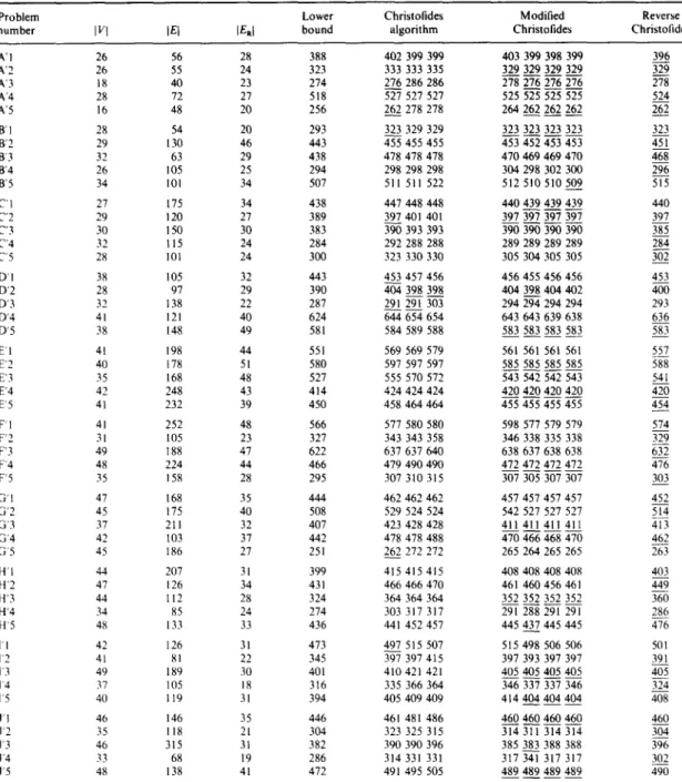
A'I 26 56 28 388 402 399 399 403 399 398 399 396 A'2 26 55 24 323 333 333 335 329 329 329 329 329 A'3 18 40 23 274 27__~6286 286 278 276 276 276 27""8 A'4 28 72 27 518 527 527 527 525 525 525 525 524 A'5 16 48 20 256 262 278 278 264262 262 262 262 B'I 28 54 20 293 323 329 329 323 323 323 323 323 B'2 29 130 46 443 455 455 455 453 452 453 453 451 B'3 32 63 29 438 478 478 478 470 469 469 470 468 B'4 26 105 25 294 298 298 298 304298 302 300 296 B'5 34 101 34 507 511 511 522 512 510 510 509 515 C'I 27 175 34 438 447448 448 440 439 439 439 440 C'2 29 120 27 389 397 401 401 397 397 397 397 397 C'3 30 150 30 383 390 393 393 390 390 390 390 385 C'4 32 t15 24 284 292 288 288 289 289 289 289 284 C'5 28 101 24 300 323 330 330 305 304 305 305 302 D'I 38 105 32 443 453 457 456 456 455 456 456 453 D'2 28 97 29 390 404 398 398 404 398 404402 400 D'3 32 138 22 287 291 291 303 294 294 294 294 293 D'4 41 121 40 624 644 654 654 643 643 639 638 636 D'5 38 148 49 581 584 589 588 583 583 583 583 583 E'I 41 198 44 551 569 569 579 561 561 561 56l 557 E'2 40 178 51 580 597 597 597 585 585 585 585 588 E'3 35 168 48 527 555 570 572 543 542 542 543 541 E'4 42 248 43 414 424 424 424 420 420 420 420 420 E'5 41 232 39 450 458 464 464 455 455 455 455 454 F'I 41 252 48 566 577 580 580 598 577 579 579 574 F'2 31 105 23 327 343 343 358 346 338 335 338 329 F'3 49 188 47 622 637 637 640 638 637 638 638 632 F'4 48 224 44 466 479 490 490 472 472 472 472 476 F'5 35 158 28 295 307 310 315 307 305 307 307 303 G'! 47 168 35 444 462 462 462 457 457 457 457 452 G'2 45 175 40 508 529 524 524 542 527 527 527 514 G'3 37 211 32 407 423 428 428 411 411 411 411 413 G'4 42 103 37 442 478 478 488 470 466 468 470 462 G'5 45 186 27 251 262 272 272 265 264 265 265 263 H'I 44 207 31 399 415 415 415 408 408 408 408 403 H'2 47 126 34 431 466 466 470 461 460 456 461 449 H'3 44 112 28 324 364 364 364 352 352 352 352 360 H'4 34 85 24 274 303 317 317 291 288 291 291 286 H'5 48 133 33 436 441 452 457 445 437 445 445 476 1'1 42 126 31 473 497 515 507 515 498 506 506 501 1'2 41 81 22 345 397 397 415 397 393 397 397 391 1'3 49 189 30 401 410 421 421 405405 405 405 405 1'4 37 105 18 316 335 366 364 346 337 337 346 324 1'5 40 119 31 394 405 409 409 414 404 404 404 408 J'l 46 146 35 446 461 481 486 460 460 460460 460 J'2 35 118 21 304 323 325 315 314 311 314 314 304 J'3 46 315 31 382 390 390 396 385 383 388 388 396 J'4 33 68 19 286 314 331 331 317 341 317 317 302 J'5 48 138 41 472 491 495 505 489 489 489 489 490

with 20 required edges, to 12 components, 49 nodes, problems are described in the following:

315 edges with 51 required edges. These Set A': 5 problems; I VGcl = 3, 16 ~< I VI ~ 28, 20 ~< IERI

Set B': 5 problems; I VGc t = 4, 26 ~<lVI ~< 34, 30 ~< IERh Set C': 5 problems; I V~cl = 5, 27 ~<lVI ~< 32, 24 ~< IERI Set D': 5 problems; I Vccl = 6, 28 ~< [ VI ~< 41,22 <~ [ERI Set E': 5 problems; IVo¢ I =7, 35~<1V1 ~<42, 39~<IERI Set F': 5 problems; I Vc=l = 8, 31 ~< I VI ~< 49, 23 ~< IERI

Set G': 5 problems; L V~I = 9, 37 ~< I VI ~< 47, 27 ~< IER[ Set H': 5 problems; I V~¢I = 10, 34 <~ I VI ~< 48, 24 ~< IERI SetI': 5problems;IV~¢l=ll,37~<lVl~<49, 18~<[ERI Set J':

5problems;IVc¢l=12,33<~lVl<<48,19<~lERI

~< 28, 40 ~< IEI ~< 72; ~<46, 54~< IEI ~ 130; ~<34, I01 ~<IE[~< 175; ~<49, 97 ~< IEI ~< 148; ~<51,168 ~<1E1<~248; ~< 48, 105 ~< IEI ~< 252; ~<40, 103<~1E1~<211; ~<34, 85 ~< IEI ~<207; ~<31, 81 ~<IEI ~< 189; ~<41,68~<1E1~<315.

(10)

Table 10. Performance comparisons of the three algorithms (50 problems)

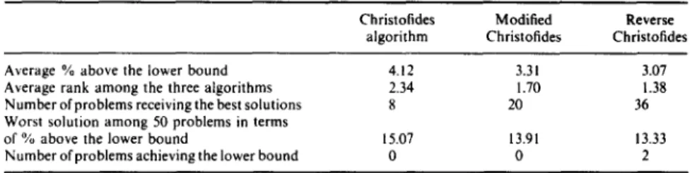
Christofides Modified Reverse algorithm C h r i s t o f i d e s Christofides Average % above the lower bound 4.12

Average rank among the three algorithms 2.34 Number of problems receiving the best solutions 8 Worst solution among 50 problems in terms

of % above the lower bound 15.07

Number of problems achieving the lower bound 0

3.31 3.07

1.70 1.38

20 36

13.91 13.33

0 2

The solutions of these 50 problems generated by the three algorithms are displayed in Table 9. Comparisons among the three algorithms in terms of average percentage above the lower bound, average rank, number of problems receiving the best solutions, worst solution in terms of percentage above the lower bound, and number of problems achieving the problem lower bound (hence the solution must be optimal), is summarized in Table 10. The results indicated that (1) the modified and reverse approaches once again outperformed the original algorithm, and (2) the reverse approach outperformed the modified algorithm.

5. CONCLUSIONS

In this paper, we considered an interesting generalization of the well-known Chinese postman problem, called the Rural Postman Problem (RPP). We first reviewed the heuristic solution procedure introduced by Christofides et al. [2], then developed two new algorithms to solve the problem approximately. The proposed two new procedures run very fast, and work well in general. We have tested them on many problems which were arbitrarily generated, and compared with the existing solution procedure (the Christofides et al. algorithm). The results indicated that the proposed two new approaches indeed improved the existing algorithm. The two new algorithms were also compared with each other, and we found that for problems with near-odd (a large proportion of odd-degree nodes) network structure, the reverse approach outperformed the modified algorithm.

REFERENCES

I. C. S. Orloff, A fundamental problem in vehicle routing. Networks 4, 35-64 (1974).

2. N. Christofides, V. Campos, A. Corberan and E. Mota, An algorithm for the rural postman problem. Imperial College Report IC-OR (1981).

3. N. Christofides, V. Campos, A. Corberan and E. Mota, An algorithm for the rural postman problem on a directed graph. Mathl Programming Study Z6, 155-166 (1986).

4. E. Benavent, V. Campos, A. Corberan and E. Mota, Analisis de heuristicos para el problema del cartero rural. Trahq/os De Estadistica Y De Investigation Operativa 36, 27-38 (1985).

5. L. Levy and L. Bodin, Scheduling in the postal carriers for the Unites States postal service: an application of arc partitioning and routing. Vehicle Routing: Methods and Studies, pp. 359-394. North Holland, Amsterdam (1988). 6. J. N. Holt and A. M. Watts, Vehicle routing and scheduling in the newspaper industry. Vehich, Routiog: Method~ aml

Studies, pp. 347-358. North Holland, Amsterdam (1988).

7. E. Beltrami and L. Bodin, Networks and vehicle routing for municipal waste collection. Networks 4, 65-94 (1974). 8. J. Desrosiers, J. A. Ferland, J. M. Rousseau, G. Lapalme and L. Chapleau, An overview of a school busing system.

Seicnt(fie Management of Transport Systems, pp. 235-243. North Holland, Amsterdam (1987).

9. R. W. Eglese and L. Y. O. Li, Efficient routeing for winter gritting. J. Opl Res. Soc. 43, 1031-1034 (1992). 10. R. W. Eglese, Routeing winter gritting vehicles. Discr. appl. Math., to appear.

11. H. I. Stern and M. Dror, Routing electric meter readers. Computers and Ops Res. 6, 209-223 (1970).

12. J. Edmonds and E. Johnson, Matching, Euler tours and the Chinese postman problem. Math. Programming 4, 88 124 (1973).

13. G. N. Frederickson, Approximation algorithms for some postman problems. J. Assoc. Computing Machinery 26, 538-554 (1979).

14. W. L. Pearn and M. L. Li, Algorithms for the windy postman problem. Computers Ops Res. 21,641-651 (1994). 15. W. L. Pearn and C. M. Liu, Algorithms for the Chinese postman problem on mixed networks. Computers Ops Res.