使用平均重疊區塊補償方法應用在H.264的時間域錯誤隱藏

(1)

國立交通大學

資訊科學與工程研究所

碩士論文

使用平均重疊區塊補償方法應用在

H.264 的時間域錯誤隱藏

A Two-Level Temporal Error Concealment method for H.264

using Average Overlapped Block Motion Compensation

研究生 : 王志銘

指導教授 : 蔡文錦教授

(2)

使用平均重疊區塊補償方法應用在 H.264 的時間域錯誤隱藏

A Two-Level Temporal Error Concealment method for H.264

using Average Overlapped Block Motion Compensation

研究生：王志銘 Student：Chih-Ming Wang 指導教授：蔡文錦 Advisor：Wen-Jiin Tsai 國立交通大學資訊科學與工程研究所碩士論文 A Thesis

Submitted to Institute of Computer Science and Engineering College of Computer Science

National Chiao Tung University in partial Fulfillment of the Requirements

for the Degree of Master

in

Computer Science

June 2007

Hsinchu, Taiwan, Republic of China

(3)

使用平均重疊區塊補償方法應用在

H.264 的時間域錯誤隱藏

學生 : 王志銘指導教授 : 蔡文錦教授國立交通大學資訊科學與工程研究所

摘要

在無線傳輸上時常會隨著頻帶的跳動而產生突發性的錯誤。而當這些錯誤發生時，常常會使傳送的封包產生錯誤。當視訊在播放時，這些錯誤的封包往往不但會造成失真也會影響到後續的影像持續錯誤。而錯誤隱藏是可以解決這個問題的方法。此篇論文中，我們主要研究在 H.264 的時間域錯誤隱藏。我們提出三種方法並將它們整合，來回復影像中的錯誤區塊。這個整合的方法主要使用兩階層式移動向量預測搭配權重式評量方式來決定遺失區塊的移動向量，最後在使用平均重疊區塊補償的方法使錯誤區塊回復更正確。 關鍵字 : 時間域錯誤隱藏、兩階層式、權重邊界、平均重疊區塊

(4)

A Two-Level Temporal Error Concealment method for

H.264 using Average Overlapped Block Motion

Compensation

Student: Chih-Ming Wang Advisor: Dr. Wen-Jiin Tsai College of Computer Science

National Chiao Tung University

Abstract

Sometimes the burst error is happened in wireless transmission due to fluctuating channel conditions. When burst-error happens, the packets may be lost. That will cause not only the degraded quality but propagate error until an I-frame arrived successfully. To avoid these situations, error concealment at decoder is often necessary.

In this thesis, we will focus on temporal error concealment in H.264. We proposed a two-level MVs prediction for choosing candidates MVs and then a weighted external boundary match algorithm as the measure criteria to determine the best MV. After the best MV is chosen, we propose a method called average overlapped block motion compensation (AOBMC) to recover the lost MB by overlapping it with multiple MBs. By combining the proposed three techniques (two-level MVs prediction, WEBMA, and AOBMC) , the experimental results show that we can recovery the lost MBs with better Peak Signal to Noise Ratio (PSNR) and visual quality.

Keywords: Temporal error concealment, Two-Level, Weighted boundary,

(5)

List of Figures

Figure 2.1 Slice groups : interleaved slice...5

Figure 2.2 Slice groups : dispersed slice ...5

Figure 2.3 Partitions of macroblock ...6

Figure 2.4 Partitions of sub-macroblock ...6

Figure 2.5 Boundary matching algorithm (BMA)...9

Figure 2.6 External Boundary matching algorithm (EBMA)...10

Figure 2.7 Selection the motion vectors for OBMC ...12

Figure 2.8 The weighting table of OBMC...13

Figure 2.9 OBMC on LEFT-UP block...13

Figure 4.1 Architecture of our method ...15

Figure 4.2 MB based prediction ...17

Figure 4.3 Sub-MB based prediction...17

Figure 4.4 First-Level Candidate MVs Selection...18

Figure 4.5 Second-Level Candidate MVs Selection ...19

Figure 4.6 Example 1 of Two-level MVs prediction...20

Figure 4.7 Example 2 of Two-level MVs prediction...21

Figure 4.8 Weighted boundary matching algorithm...22

Figure 4.9 Example of WEBMA...23

Figure 4.10 Selection the motion vectors for AOBMC ...24

Figure 4.11 AOBMC on LEFT-UP Sub-MB ...25

Figure 4.12 Example of AOBMC ...26

Figure 5.1 The Result of Two-Level MVs prediction ...30

Figure 5.2 The Result of WEBMA...31

Figure 5.3 The Result of AOBMC...33

Figure 5.4 Result of combined method ...34

Figure 5.5 Example 1 of combined method ...35

(7)

(8)

1. INTRODUCTION

Video transmission over wireless networks is more popular now because of more and more portable consumer devices such as mobile phone, PDA, and so on. But sometimes the burst error is happened in wireless transmission due to fluctuating channel conditions. When burst-error happens, the packets may be lost. That will cause not only the degraded quality but propagate error until an I-frame arrived successfully. To avoid these situations, error resilience at encoder and error concealment at decoder are often necessary.

Error concealment methods are not defined in H.264 standard. This means that the decoder can explore various algorithms to make a better result. Error concealment methods can be divided into three categories, spatial error concealment [1][9][11][14][16] , temporal error concealment [1]-[2][4]-[8][10-13][15], and frequency domain error concealment [5]. In this thesis, we will focus on temporal error concealment only. The basic idea of temporal error concealment is to estimate missing motion vectors (MVs) for lost macroblock (MB) and then use them to find a good macroblock in the reference frame to replace the lost MBs. Some methods have been proposed to choose candidate MVs and judge the best one based on some measure criteria [6][12][13]. For candidates MVs selection, many conventional methods choose the MVs of the collocated MB, median or average of surrounding MVs of lost MBs, zero motion vector, the MVs of neighboring MBs and even MVs of extrapolation [13]. For measure criteria, Boundary matching algorithm (BMA) [13] is most widely used, which relies on the idea that the contiguous pixels in an

(9)

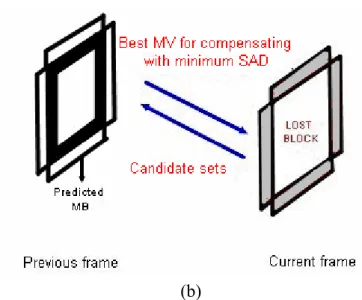
image are highly correlated. By using BMA, the pixels in the external boundary of the lost MB and the pixels in the internal boundary of the predicted MB are used to compute the Sum of Absolute Difference (SAD) as the measure criteria. Among multiple predicted MBs (pointed by candidate MVs), the one with minimum SAD will be selected. In BMA, while it is good for smooth, it did not work well when there are tilting edges across macroblock boundary. An inappropriate BMA result will mislead the judgment process and determine an incorrect candidate MV for error concealment. For this reason, some research have proposed external boundary matching algorithm (EBMA) [6], as measure criteria. EBMA relies on the idea that the external boundary of the lost MB should appear in the reference frame. This idea has been proved in some literatures.

ITU-T H.264 develops the latest standard in which some new coding scheme are adopted. One of the major differences with the other previous coding standards is the motion estimation. In H.264, the motion estimation with vary block sizes will increase the quality of the video stream. The standard also supports multiple slice groups (described in previous versions of the draft standard as Flexible Macroblock Ordering or FMO). The concept of them can help to make the error concealment more effective because more information around the best MB is available for prediction.

The overlapped block motion compensation (OBMC) defined in [3] is a good solution for motion compensation because it not only increases prediction accuracy but also avoids blocking artifacts. The [8] has proved that applying OBMC in error concealment can improve the visual quality.

(10)

However, OBMC has high computation complexity and, when applying to error concealment, the unequal weighting values for three overlapped blocks may lead to inappropriate prediction.

In this thesis, we proposed a two-level MVs prediction for choosing candidates from MVs and then a weighted external boundary match algorithm as the measure criteria to determine the best MV. Once the best MV is chosen, the predicted MB for recovering the lost MB is conducted by overlapping it with multiple MBs. A method called average overlapped block motion compensation (AOBMC) is proposed for this purpose. By combining the proposed three techniques (Two-level MVs prediction, WEBMA, and AOBMC) , the experimental results show that we can recovery the lost MBs with better Peak Signal to Noise Ratio (PSNR) and visual quality.

The thesis is organized as follows. First, we describe some conventional error concealment algorithms and some schemes of the H.264 in section 2. The motivation and proposed methods are presented in section 3 and 4, respectively. Finally, we will show the experimental results in section 5, and conclude this thesis in section 6.

(11)

2. RELATED WORK

About this section, we will describe some methods which we will adopt. First, we will introduce dispersed slice and inter prediction in H.264. Then we will introduce the selection of candidate sets for MVs, and some measure criteria for predicting the lost MVs. Finally, the OBMC will be described.

2.1. Dispersed Slice

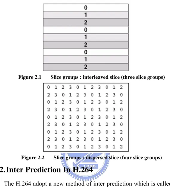
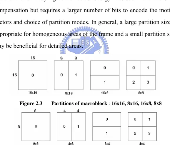
A slice group is a subset of MBs in a coded picture and may contain one or more slices. MBs are coded in raster scan within each slice in a slice group. The allocation of MBs is determined by a macroblock to slice group map that indicates to which slice group each MB belongs. Interleaved and dispersed slice are two types of macroblock-to-slice group map. Both of them have a great benefit for temporal error concealment.

For a damaged or lost MB, a better concealment can be achieved if there are more correctly reconstructed MBs around it. In interleaved slice (figure 2-1), if one slice is lost, the MVs of top and bottom macroblocks which belong to different slices can be used to predict each lost MB. In dispersed slice (figure 2-2), if one slice is lost, we can use the MVs of top, bottom, left, right MBs for error concealment.

(12)

Figure 2.1 Slice groups : interleaved slice (three slice groups)

Figure 2.2 Slice groups : dispersed slice (four slice groups)

2.2. Inter Prediction In H.264

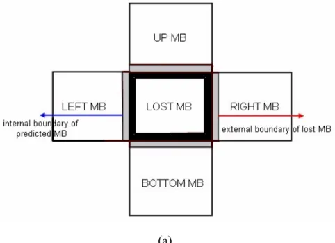
The H.264 adopt a new method of inter prediction which is called as “tree structured motion compensation”. When such prediction is used, we can have a number of combinations of sub-blocks with various sizes within each macroblock for motion compensation. In figure 2.3, we can see that the luminance component of each macroblock (16×16 samples) may be partitioned up in four ways : one 16×16 macroblock partition, two 16×8 partitions, two 8×16 partitions or four 8×8 partitions. If the 8×8 mode is chosen, each of the four 8×8 sub-macroblocks within the macroblock may be further partitioned four ways as shown in Figure 2.4. They are one 8×8 sub-macroblock partition, two 8×4 sub-macroblock partitions, two 4×8 sub-macroblock partitions or four 4×4

(13)

sub-macroblock partitions.

A separate motion vectors is required for each partition or sub-macroblock. All the motions vectors and the choice of partition modes must be encoded in the compressed bitstream. If we choose a sub-block of large partition size, which means that a small number of bits are required to encode less number of motion vectors and signal the mode of partition but the compensated residual may contain a significant amount of energy in frame areas with high detail. Choosing a small partition size may give a lower-energy residual after motion compensation but requires a larger number of bits to encode the motion vectors and choice of partition modes. In general, a large partition size is appropriate for homogeneous areas of the frame and a small partition size may be beneficial for detailed areas.

Figure 2.3 Partitions of macroblock : 16x16, 8x16, 16x8, 8x8

Figure 2.4 Partitions of sub-macroblock : 8x8, 4x8 8x4, 4,4

2.3. Candidate Motion vector

For the temporal error concealment, a large number of researches have been proposed on selecting as many as candidate MVs to predict the

(14)

lost MV. The surrounding MVs of the lost MB are the most popular. Of course, some derived MVs like average MV or median MV, as well as zero-motion MV are also widely used. Some researches even use the MVs which are explored from previous frames or backward frame [1][4].

2.4. Criteria of measure

This chapter we will introduce some conventional methods for measure which candidate is best for compensating. There are called as Boundary matching algorithm and external boundary matching algorithm. In some proposed, it have proved that using EBMA to measure is more efficient than BMA.

2.4.1. Boundary matching Algorithm

Boundary matching Algorithm (BMA) is a measure criterion for

judging the best MV among the candidate MVs to recover the lost MB. It has been adopted by in JM (Joint Model) software. BMA is based on the idea that the contiguous pixels in an image are highly correlated, so the external boundary of the lost MB may have a minimum variation with the internal boundary of the predicted MB. In other words, BMA prefers a MB which can replace the loss MB with smooth boundary connectivity with adjacent MBs.

Figure 2.5 illustrates the pixels that will be used by BMA for calculation. Assume the MB in the center is a predicted MB, the pixels located inside the dark are (one pixel width) are called internal boundary of the predicted MB; while the pixels inside the grey area (also one pixel width) are called the external boundary of the lost MB.

(15)

between the corresponding pixels in these two areas. The formula of SADBMA is given below.

1

the difference on up boundary

the difference on bottom boundary

// // ( ( , 1) '( ' , ') ( ( , 1) '( ' , ' ) ( ( 1, ) '( ', N i N i BMA SAD f x i y f x i y f x i y N f x i y N f x y i f x = = = + − − + + + + − − + + + − + −

∑

1 1

the difference on left boundary

the difference on right boundary

// // ' ) ( ( 1, ) '( ' , ' ) N i N i y i f x N y i f x N y i = = + + + − + − + +

∑

Where f is the luminance of current frame, and f’ is the luminance of previous frame. (x, y) is the position of the left-up corner pixel on the lost MB and (x’, y’) is the position of the predicted MB from candidate MV shifted with (x, y).

Figure 2.5(b) shows that for each MV in the candidate set, we will have predicted MB for SADBMA calculation. The one with minimum

SADBMA is the best candidate and will be selected to recover the lost MB.

(16)

(b)

Figure 2.5 Boundary matching algorithm (BMA)

2.4.2. External boundary matching algorithm

External boundary matching algorithm (EBMA) is based on the

idea that external boundary of lost macroblock may appear in previous frame so that the external boundary of the lost MB may have a minimum variation with the external boundary of predicted MB. Some researches methods have proved that EBMA is better than BMA, because the BMA sometimes will have wrong prediction when there are tilting edges across boundary. With EBMA, SAD is calculated with the pixels on the external boundary of the lost MB and the pixels on external boundary of predicted MB with corresponding position.

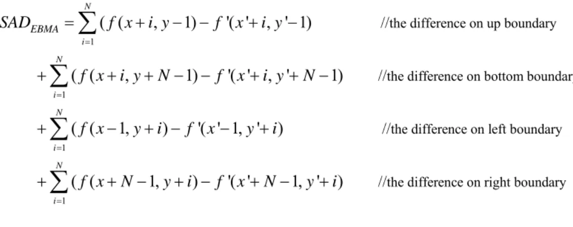
SADEBMA is defined as the Sum of the Absolute Difference (SAD)

between the corresponding pixels in these two external boundaries. The formula of SADEBMA is given below.

(17)

1

the difference on up boundary

the difference on bottom boundary // // ( ( , 1) '( ' , ' 1) ( ( , 1) '( ' , ' 1) ( ( 1, ) '( ' 1, N i N i EBMA SAD f x i y f x i y f x i y N f x i y N f x y i f x = = = + − − + − + + + − − + + − + − + − −

∑

1 1

the difference on left boundary

the difference on right boundary // // ' ) ( ( 1, ) '( ' 1, ' ) N i N i y i f x N y i f x N y i = = + + + − + − + − +

∑

Where f is the luminance of current frame, and f’ is the luminance of previous frame. (x, y) is the position of the left-up corner pixel on the lost MB and (x’, y’) is the position of the predicted MB from candidate MV shifted with (x, y).

Figure 2.6 shows that among the candidate MVs, we will judge the one with minimum SADEBMA to recover the lost MB.

Figure 2.6 External Boundary matching algorithm (EBMA)

2.5. Overlapped Block Motion Compensation

(18)

H.263 Annex F Advanced Prediction mode, is a technique originally designed for use in the motion estimation of the encoding process. It not only increases prediction accuracy, but also avoids blocking artifacts. With OBMC, each pixel in an 8x8 luminance prediction block is a weighted sum of three prediction values, divided by 8 (with rounding). In order to obtain the three prediction values, three motion vectors are used:

z The motion vector of the current luminance block

z The motion vector of the block at the left or right side of the current luminance block

z The motion vector of the block above or below the current luminance block.

For each pixel, in addition to the motion vector of current MB, the motion vectors of the blocks at the two nearest block borders are used. This means that for the upper half of the block the motion vector corresponding to the block above the current block is used, while for the lower half of the block the motion vector corresponding to the block below the current block is used. Similarly, for the left half of the block the motion vector corresponding to the block at the left side of the current block is used, while for the right half of the block the motion vector corresponding to the block at the right side of the current block is used.

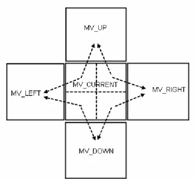
Figure 2.7 shows that for each pixel of LEFT_UP luminance prediction 8x8 sub-MB, the motion vectors (MV_CURRENT, MV_UP, and MV_LEFT) are used. Similar rules are applied in the other sub-MBs in macroblock.

(19)

Figure 2.7 Selection the motion vectors for OBMC.

For each pixel, P i j( , ), in an 8*8 luminance prediction block is

governed by the following equation:

0 1 2

( , ) ( ( , ) ( , ) ( , ) ( , ) ( , ) ( , ) 4) / 8

P i j = q i j ×H i j +r i j ×H i j +s i j ×H i j +

Where, , , and are the pixels from the referenced

picture as defined by ( , ) q i j r i j( , ) s i j( , ) 0 0 1 1 2 2 ( , ) ( , ) ( , ) ( , ) ( , ) ( , ) x y x y x y q i j p i MV j MV r i j p i MV j MV s i j p i MV j MV = + + = + + = + + Here, ₍ 0_, 0₎ x y

MV MV means the motion vector of the current block,

1 1

(MV MV_x, _y) means the motion vector of the block either above or below,

and ₍ 2_, 2₎

x y

MV MV denotes the motion vector of the block either left or

right.

(20)

(b), and (c) as below.

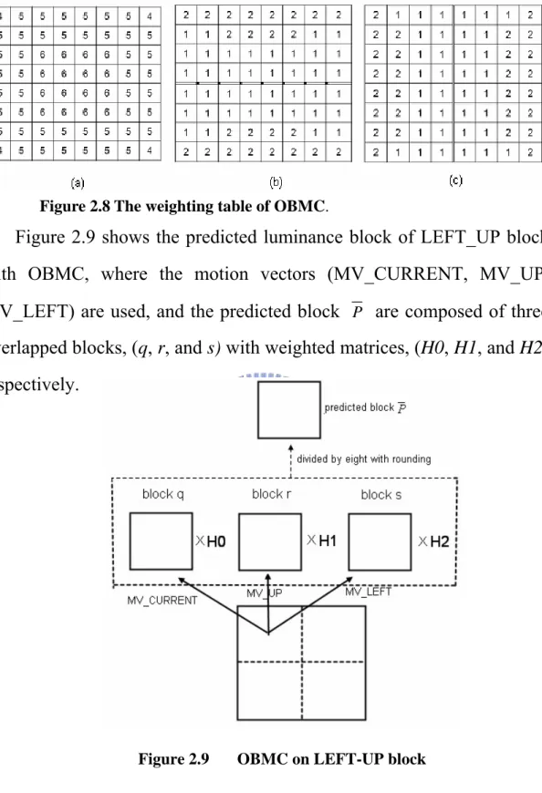
Figure 2.8 The weighting table of OBMC.

Figure 2.9 shows the predicted luminance block of LEFT_UP block with OBMC, where the motion vectors (MV_CURRENT, MV_UP, MV_LEFT) are used, and the predicted block P are composed of three

overlapped blocks, (q, r, and s) with weighted matrices, (H0, H1, and H2), respectively.

(21)

3. MOTIVATION

The key issues of temporal error concealment are 1: how to select

candidate MVs and 2: how to judge which one is best for compensating

the lost MBs. A large number of researches have been proposed on selecting candidate MVs as many as possible, and choose the best one among them according to some measure criteria for compensating the lost MBs. However, some research results have found that having more candidate MVs might not help finding the best matched MB because an unrelated candidate MV might still get the best score by applying unreliable measure criteria which uses inappropriate boundary information.

Base on this observation, recent researches tend to split a lost 16x16 MB into four 8x8 Sub-MBs. For each of these Sub-MBs, they will choose those MVs which are most close to it (neighboring MVs) as candidates only. By excluding the MVs that are far from the lost Sub-MB in spatial distance, measure criteria is applied on fewer but more likely candidates to find the MB for concealment . However, sometimes the best MV for the lost Sub-MB is one of the surrounding MVs of the lost MB, but not the neighboring MV. For this reason, we have developed a two-level MVs prediction method which will pick up significant MVs among all the surrounding MVs as candidate set only. We also proposed a weighted EBMA method which explores more reliable boundary information as measure criterion so that the more accurate MVs can be found. Finally, we also proposed an average overlapped block motion compensation method (called as AOBMC) for recovering the lost MBs more accurately.

(22)

4. THE PROPOSED METHOD

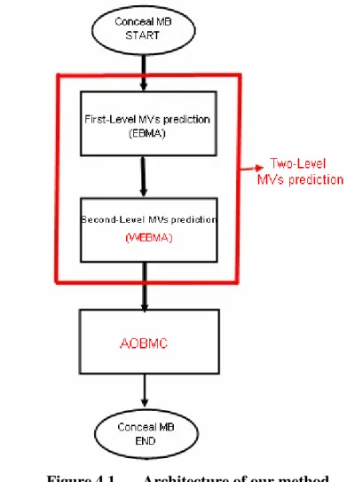
Figure 4.1 shows architecture of our method for temporal error concealment. In this section, we will explain the method of Two-Level MVs prediction, weighting external boundary matching algorithm

(WEBMA), and average overlapped block motion compensation

(AOBMC).

Figure 4.1 Architecture of our method

4.1. Two-Level MVs prediction

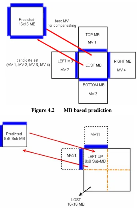
The proposed two-level MVs prediction is based on the 8x8 Sub-MB. The major difference of using 16x16 MB and the 8x8 Sub-MB are candidate set selection and the boundaries used in measure criteria. Figure 4.2 shows the example, where MB-based prediction uses four

(23)

surrounding MVs (MV1, MV2, MV3, MV4)as candidate set and the four

boundaries (shown in gray level) are used with EBMA. Figure 4.3 shows that the Sub-MB based prediction uses two neighboring MVs (e.g. MV11

and MV12 for left-top Sub-MB) as candidate set and the two boundaries

in grey area are used with EBMA. As an alternative to two-neighboring MVs, eight-surrounding MVs which are close to 16x16 MB as candidates in Sub-MB based prediction can also be found in some literatures. Of course, some derived MVs like average MV or median MV, as well as zero-motion MV which are not shown in the example are also widely used.

As described above, there are two-alternatives for candidate selection for Sub-MB based prediction; one is two-neighboring MVs and the other is eight-surrounding MVs. In general, the selection between them is a trade-off between complexity and accuracy. Two-neighboring MVs is only a sub set of eight-surrounding MVs, and it should not outperform eight-surrounding MVs, which improves the accuracy by increasing the computation complexity for handling more candidates. However, it is not always the case that eight-surrounding MVs performs better than two-neighboring MVs as the example shown later in this section. The two-level MVs prediction method we present here tries to find the best MV between these two methods, however, with the computation complexity less than eight-surrounding MVs prediction.

(24)

Figure 4.2 MB based prediction

Figure 4.3 Sub-MB based prediction

In the two-level MVs prediction, we first apply two neighboring MVs prediction to pick up four significant MVs from eight surrounding MVs, and then the best one is selected among these significant MVs.

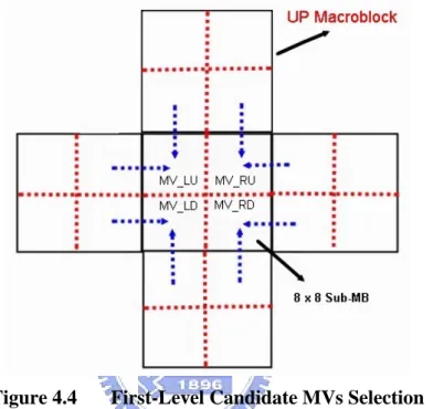
The candidates for first level motion vector of LEFT-UP Sub-MB are the MV of LEFT_DOWN 8x8 Sub-MB of the above MB, and the MV of RIGHT-UP 8x8 Sub-MB of the left MB. Similar rules can be applied to find candidates for all the other Sub-MBs, as shown in Figure 4.4 below,

(25)

where each Sub-MB has two candidates in first level. Then we apply EBMA measure criterion on the three candidates for each Sub-MB, such that a single candidate MV is obtained for each Sub-MB. We call such MVs as significant MVs denoted by MV_LU, MV_RU, MV_LD, and MV_RD respectively.

Figure 4.4 First-Level Candidate MVs Selection

Second-level MVs prediction uses the result of first-level prediction, that is, the significant MVs, as more candidates to find the best MB for concealment. Figure 4.5 shows the second-level candidate MVs for each Sub-MB, where figure 4.5(a) shows that, in addition to the significant MV predicted from first-level, LEFT_UP Sub-MB will include three more MVs (MV_RU, MV_LD, MV_RD) to candidate set in the second level prediction. The same rules also apply to the other three Sub-MBs as shown in Fig 4.5(b), (c), and (d), respectively. The measure criterion on second-level prediction is different with that used in the first level. In second-level, we will adopt WEBMA (described in the next section) to measure so the best one is obtained for each Sub-MB.

(26)

(a) LU (a) RU

(a) LD (a) RD

Figure 4.5 Second-Level Candidate MVs Selection

Figure 4.6 shows an example of concealment result using

stream-mobile, where figure 4.6(a) is the original frame which is reconstructed by the decoder when no MB is damaged, figure 4.6(b) shows the damaged frame which has one slice loss. Figure 4.6(c), (d), and (e) show the concealment results when different methods : two-neighboring MVs prediction, eight-surrounding MVs prediction, and two-level MVs prediction are used, respectively. The result shows that the two-neighboring MVs prediction performs better than eight-surrounding MVs prediction in this example and the proposed two-level MVs prediction performs similar to two-neighboring MVs prediction.

(27)

Figure 4.6Example 1 of Two-level MVs prediction. The PSNR is calculated between center concealed MB and error-free MB.

Figure 4.7 shows the example of another frame in the same stream-mobile. In this case, eight-surrounding MVs prediction outperforms two-neighboring MVs prediction and the proposed two-level MVs prediction has similar result to eight-surrounding MVs prediction.

From the two examples above we can observe that the proposed two-level MVs prediction achieve the result close to the better one of the other two methods.

(28)

Figure 4.7Example 2 of Two-level MVs prediction. The PSNR is calculated between center concealed MB and error-free MB.

4.2. Weighted external boundary matching algorithm

External boundary matching algorithm (EBMA) has been proposed in some researches, and it has been proved that, when applied to temporal error concealment, it is better than boundary matching algorithm (BMA). Our measure criterion also chooses EBMA to be based upon. However, since Sub-MB based prediction uses only two boundaries, rather than four boundaries, a lot of information is lost in judging the best MV candidate. As figure 4.3 shows, using Sub-MB prediction in EBMA, only 8x1x2 pixels are calculated for each candidate MV. In other word, only one corner of the lost MB is considered. We think one corner information is too less to judge the best MV of each Sub-MB.

In the proposed weight external boundary matching algorithm (WEBMA), we add more boundary information in the measure criteria to judge the best MV. Figure 4.8 shows that the SAD for each Sub-MB, is composed of three components: one corner information from the Sub-MB being considered, and the two corners information from two adjacent Sub-MBs

The SAD, SADWEBMA(Sub-MB), of each Sub-MB is governed by the

following equation：

WEBMA Sub-MB EBMA C EBMA V EBMA H

SAD ( ) = SAD ( )* + SADα ( )* + SADβ ( )* γ

Here, SADWEBMA(C) denotes the Sum of Absolute Difference on

boundary pixels of the current Sub-MB, SADWEBMA(V) denotes that of the

(29)

Sub-MB either to the left or right of current Sub-MB. The α, β, and γ are the weighted factor in each SAD. In figures 4.8(a) shows that the SAD on LEFT-UP Sub-MB in each MV of candidate set ,and the SADWEBMA

composed of the SAD of self, below, and right Sub-MB. Similar rule also can be applied to the other sub-MBs, as shown in Figure 4.8(b), (c), and (d), respectively. In two-level MVs prediction, the WEBMA is adopted on second level, because the predicted MVs on second level are more significant.

(a) SAD of LEFT-UP Sub-MB (b) SAD of RIGHT-UP Sub-MB

(c) SAD of LEFT-DOWN Sub-MB (d) SAD of RIGHT-DOWN Sub-MB

Figure 4.8 Weighted boundary matching algorithm

(30)

stream-mobile. It is observed that if we only adopt EBMA, the result of using two-neighboring MVs, eight-surrounding MVs, and even two-level MVs will generate the same date number, 4, twice on the calendar as shown in figure 4.9(c), (d), and (e), respectively . However, by adopting WEBMA, we can reconstruct the right date numbers, 4 and 5 as shown in figure 4.9(f), and the visual quality after concealment is also better than that of using EBMA.

Figure 4.9Example of WEBMA. The PSNR is calculated between center concealed MB and error-free MB.

4.3. Average Overlapped Block Motion Compensation

After predicting the MVs for lost MB, some methods have been developed to further improve the concealment quality based upon the predicted MVs, rather than directly copying the pointed Sub-MB in the reference frame to replace the lost Sub-MB only. Overlapped motion block compensation (OBMC) is proposed to be applied on error concealment for this purpose [8], where each lost block is recovered by. Three overlapped blocks with a large weighted value on current block.

(31)

However, we think the OBMC which is originally developed for motion compensation cannot be applied to error concealment directly because the predicted MV for the lost block may not be accurate. For this reason, our method is to adopt the average overlapped block motion compensation (AOBMC).

The AOBMC is composed of five overlapped blocks and every overlapped block has the same weighting. Figure 4.10 shows the example of five motion vector selection in AOBMC for LEFT-UP Sub-MB. In addition to the predicted MV for the current Sub-MB, the motion vectors of the up, bottom, left and right block are also considered.

Figure 4.10 Selection the motion vectors for AOBMC

For each pixel, P i j( , ), in an 8*8 luminance prediction block, it’s value is governed by the following equation:

( , )

[( ( , )

( , )

( , )) / 5]

P i j

=

round c i j

+

u i j

+

b i j

+

l i j

+

r i j

Where , , , and are the pixels from the referenced picture as defined by

( , )

(32)

( , )

(

,

)

( , )

(

,

)

( , )

(

,

)

( , )

(

,

)

( , )

(

,

)

c c x y u u x y b b x y l l x y r r x y

c i j

p i MV

j MV

u i j

p i MV

j MV

b i j

p i MV

j MV

l i j

p i MV

j MV

r i j

p i MV

j MV

=

+

=

+

=

+

=

+

=

+

Here, ( c, ) c x y

MV MV means the motion vector of the current block,

( u, )

u x y

MV MV and (MV_xb,MV_yb) mean the motion vectors of the above and

below block.( l, )

l x y

MV MV and (MV_xr,MV_yr) denotes the motion vector of

the left and right block.

Figure 4.11 shows the predicted luminance block for LEFT_UP Sub-MB on AOBMC, where five motion vectors (MV_CURRENT, MV_UP, MV_DOWN, MV_LEFT, and MV_RIGHT) are used, and the predicted block P are the average of the five overlapped blocks. Similar

rules are also applied on the other Sub-MB for compensation.

(33)

Figure 4.12 shows an example of concealment result using stream-foreman, where figure 4.12(a) is the original frame which is reconstructed by the decoder when no MB is damaged, figure 4.12(b) shows the damaged frame which has one slice loss and is recovered with Two-level MVs prediction without OBMC or AOBMC, figure 4.12(c) and figure 4.12(d) show the result with OBMC and AOBMC, respectively. We can observe that it has effect of smooth on recovering the lost MB by using OBMC and AOBMC and the quality of AOBMC is better than OBMC.

(a) Error Free (b) Two-level +WEBMA (PSNR=35.94)

(c) Two-level + WEBMA (OBMC) (d) Two-level +WEBMA(AOBMC) (PSNR=37.54) (PSNR=36.82)

(34)

From the point of computation, it is observed that the OBMC need more computation than AOBMC. The OBMC needs 3x8x8 multiplications, 2x8x8 additions, and 8x8 divisions, but the AOBMC needs only 4x8x8 additions, and 8x8 divisions. By AOBMC, the better visual quality can be achieved with reduced computation complexity.

(35)

5. EXPLEMENT AND RESULT

A number of test streams of QCIF (176x144) resolution were used in the performance evaluation. Every test pattern is coded as “IBBP” GOP structure of motion compensation video coding so that a P-frame with partial loss is recovered by the reference I-frame. In other words, the process is applied using a reference frame that is three frames ahead of the current frame. In the experiments, this process is repeated for 50 frames of each sequence. Every P-frame is coded as dispersed slice with two slice groups. The inter prediction is adopted and the Sub-MB of 16x16, 8x16, 16x8, and 8x8 sub-MB are used. QP=28 is used. The damaged frame is generated by dropping one slice.

The experiments use the PSNR for measuring the quality of the concealed frame. The formula of Peak Signal to Noise Ratio (PSNR) is defined as below: 2

255 10 log

PSNR

MSE

⎛

⎞

= ×

_⎜

_⎟

⎝

⎠

Here, MSE means the mean square error and formula is defined as:

2 1 1 1

( ( , )

( , ))

height Framesize width n n n i j

I i j

P i j

MSE

FrameSize

= = =

−

=

∑ ∑ ∑

Here, I is the value of the pixels in original frame and P is value of pixels in processed frame.

For the performance comparison, we will divide them into four sections for examination, including the effectiveness of two-level MVs

(36)

prediction, WEBMA, and AOBMC. Finally, we will investigate the performance of the combination of the proposed two-level prediction, WEBMA, and AOBMC.

5.1. Two-level MVs prediction

Figure 5.1(a) and figure 5.1(b), show the PSNR (between concealed frame and error-free frame) of streams “mobile and “foreman”, respectively, after error concealment. It is observed that sometimes the two-neighboring MVs prediction is better than eight-surrounding MVs prediction, and sometimes it is not. However, the PSNR of the two-level MVs prediction is close to the better one of two-neighboring and eight-surrounding MVs prediction. Many performance comparisons about two-level MVs prediction are also experimented in many other test streams, and the effects are proved.

(37)

(b) “foreman” stream

Figure 5.1 The Result of Two-Level MVs prediction

5.2. Weighted external boundary matching algorithm

As shown in figure 5.1(a) and figure 5.1(b), the PSNR of eight-surrounding MVs prediction performs better than two neighboring MVs prediction in most of the cases, therefore, we will use it for comparison later. To evaluate the performance of the proposed WEBMA, three methods are compared, they are eight-surrounding MVs prediction with EBMA, two-level MVs prediction with EBMA, and two-level MVs prediction with WEBMA. The α,β,γ of the WEBMA are adopted as 0.6, 0.2, 0.2 for testing.

Figure 5.2 shows the result of test steams “mobile”, and “foreman”. We observed that the effect of using WEBMA in mobile stream is more

observable than that in foreman stream. Although the performance improvement is not significant in “foreman” stream, it is not degraded

(38)

either. To sum up, the WEBMA is better than conventional EMBA to predict MV more accurately.

(a) “mobile”

(a) “foreman”

(39)

5.3. Average Overlapped block motion compensation

To evaluate the performance of AOBMC, three methods based on two-level MV prediction with WEBMA are used : one with AOBMC, one with conventional OBMC, and the other one without AOBMC and OBMC. Figure 5.3(a) shows that the result of using AOBMC in “mobile” is significantly better compared to that using the OBMC (average PSNR up to 0.55 dB) and that without OBMC (up to 1.21 dB). Figure 5.3(b) (“foreman”) shows the result of using AOBMC is increased up to 0.35 dB compared that of OBMC and up to 1 dB compared with that of without OBMC.

(40)

(b) “foreman”

Figure 5.3 The Result of AOBMC

5.4. Combined method

After evaluating the effectiveness of the two-level MVs prediction, WEBMA, and AOBMC, separately, here, we evaluate the performance of the combination of these three methods (Two-level MVs prediction + WEMBA + AOBMC). The comparison is made between the combined method and the eight-surrounding MVs prediction with EBMA as well as the conventional eight-surrounding MVs prediction with BMA. Figure 5.4 shows the result of comparison for difference test streams compared with the other two methods, the proposed method has the average PSNR improvement up to 1.66db for “mobile” stream and up to 1.11 dB for “foreman” stream.

(41)

(a) “mobile”

(b) “foreman”

Figure 5.4 Result of combined method

Figure 5.5 shows an example of concealment result using stream-foreman, where figure 5.5(a) is the original frame which is reconstructed by the decoder when no MB is damaged, figure 5.5(b), and (c) shows the damaged frame which has one slice loss and is recovered with BMA and EBMA with eight-surrounding MVs prediction, figure 5.5(d) shows the damaged frame which is recovered with WEBMA with

(42)

two-level MVs prediction, and figure 5.5(e) show the effect of our combined method. We observe that our combined method can reduce the blocking artifacts and improve the quality.

(a) Error Free (b) Eight-surrounding with BMA (PSNR=34.53)

(c) Eight-surrounding with EBMA (d) Two-level with WEBMA

(PSNR=35.15) (PSNR=35.94)

(e) Combined Method (PSNR=37.54)

Figure 5.5 Example 1 of combined method

Figure 5.6 shows an example of concealment result using carphone-stream, where figure 5.6(a) is the original frame which is

(43)

reconstructed by the decoder when no MB is damaged, figure 5.6(b) shows the damaged frame which is recovered with WEBMA with two-level MVs prediction, and figure 5.6(c) show the effect of our combined method. We observe that although using AOBMC sometimes generates some error, it still has effect of smooth for recovering the lost MB and overall PSNR is also improved by using our combined method.

(a) Error Free (b) Two-level with WEBMA (PSNR=34.23)

(c) Combined Method (PSNR=35.99)

Figure 5.6 Example 2 of combined method

Figure 5.7 shows the experimental results for more test streams. The effect of our combined method is better than using conventional eight-surrounding MVs prediction with BMA and eight-surrounding MVs prediction with EBMA.

(44)

Test Stream Combined method Eight surrounding (EBMA) Improved PSNR Eight surrounding (BMA) Improved PSNR Mobile 30.9328 29.2695 1.6633 28.6103 2.3225 Foreman 39.2995 38.1886 1.1109 35.9398 3.3597 Mother & daughter 42.5710 41.1341 1.4369 40.8303 1.7407 Carphone 36.0224 34.7268 1.2956 33.8600 2.1624 Salesman 36.4215 35.5329 0.8886 34.4564 1.9651 Claire 42.4019 40.8944 1.5075 39.3500 3.0519 America 43.5277 41.9955 1.5322 41.0492 2.4785

(45)

6. CONCLUSION AND FUTURE WORKS

We have presented our proposed methods for temporal error concealment. For the candidate selection in the two-level MVs prediction, we choose the significant MVs by EBMA in first level, and using them by adopting WEBMA to determine the best MV for recovering the lost MB in second-level. Two-level MVs prediction not only costs small complexity, but also have better effectiveness than two-neighboring MVs prediction and eight-surrounding MVs prediction. For measuring criteria, when using EBMA in Sub-MB based prediction, only 8x1x2 pixels are calculated for each candidate MV. Our proposed WEBMA adds more boundary information for measuring criterion, and we have shown that it has better quality than that of using EBMA. Finally, for recovering the lost MB more accurately, the result of adopting AOBMC has presented that it not only has lower complexity but also better effectiveness than that of adopting OBMC.

By combing our proposed methods, which are two-level MVs prediction, WEMBA, and AOBMC, respectively, we can get better performance than using conventional eight-surrounding MVs prediction with BMA and eight-surrounding MVs prediction with EBMA. The experiment results also show that our combined method is an adaptive technique for temporal error concealment in H.264.

In the future, we plan to find the better weighting value for judging the best MV for each lost sub-MB dynamically, and enhance the AOBMC to prevent that we will select the bad MVs for overlapping. The intra-coded MBs may also appear in the P-frame when there have high

(46)

spatial-correlation in the MB, or scene-changing between the frames. If the surrounding MBs of the lost MB are intra-coded in most part, it shows that recovering the lost MB by spatial error concealment may be better. Finally, we will research the mode decision for concealing the P-frame to do temporal or spatial error concealment.

(47)

REFRENCE

[1] Agrafiotis, D. Bull, D.R. Canagarajah, C.N. “Enhanced Error Concealment With Mode Selection”, IEEE Trans. on Circuits and Systems for Video Technology, vol. 16, pp. 960- 973, Aug. 2006. [2] Donghyung Kim, Siyoung Yang, and Jechang Jeong, “A New

Temporal Error Concealment Method for H.264 using Adaptive Block Sizes”, Image Processing, 2005. ICIP 2005. IEEE International Conference. Vol. 3, pp. III- 928-31, Sept. 2005.

[3] ISO/IEC 14496-2:2001. Streaming Video Profile, 2001.

[4] Jae-Young Pyun, Jun-Suk Lee, Jin-Woo Jeong, Jae-Hwan Jeong and Sung-Jea Ko, “Robust Error Concealment for Visual Communication in Burst-Packet-Loss Networks”, IEEE Transactions on Consumer Electronics, Vol. 49, No. 4, pp. 1013-1019, Nov. 2003.

[5] Jae-Won Suh, Yo-Sung Ho, “Error concealment based on directional interpolation”, IEEE Trans. on Consumer Electronics, vol. 43, pp. 295-302, Aug. 1997.

[6] J. Zhang, J. F. Arnold, and M. R. Frater, “A cell-loss concealment technique for MPEG-2 coded video”, IEEE Trans. Circuits on Circuits and Systems for Video Technology, vol. 10, no. 4, pp. 659–665, Jun. 2000.

[7] Ming-Chieh Chi, Mei-Juan Chen, Jia-Hwa Liu, Ching-Ting Hsu: “High performance error concealment algorithm by motion vector refinement for MPEG-4 video”, IEEE International Symposium on Circuits and Systems, vol. 3, pp. 2895-2898, May. 2005.

(48)

[8] M.J. Chen, L.G. Chen, and, R.M. Weng, " Error concealment of lost motion vectors with overlapped motion compensation", IEEE Trans. on Circuits and Systems for Video Technology, vol. 7, no. 3, pp. 560-563, June 1997 (SCI & EI).

[9] O. Nemethova, A. Al Moghrabi, M. Rupp, “Flexible Error Concealment for H.264 Based on Directional Interpolation”, in Proc. Proceedings of the 2005 International Conference on Wireless Networks Communications and Mobile Computing, vol. 2, pp. 1255-1260, June, 2005.

[10]Pei-Jun Lee, Homer Chen, and Liang-Gee Chen, “A New Error

Concealment algorithm for H.264 Video Transmission”, International Symposium on Intelligent Multimedia, Video & Speech Processing, Hong-Kong, pp. 619-622 Oct. 2004.

[11]S. Belfiore, M. Grangetto, E. Magli, G. Olmo, ``Spatio-temporal video error concealment with perceptually optimized mode selection”, ICASSP 2003 - IEEE International Conference on Acoustics, Speech, and Signal Processing, vol. 5, pp. 748-751 Apr. 2003.

[12]T. Chen, X. Zhang, and Y.Q. Shi, "Error concealment using refined boundary matching algorithm", Proc. ITRE, pp.55–59, Aug. 2003. [13]W.-M. Lam, A. R. Reibman, and B. Liu, ``Recovery of lost or

erroneously received motion vectors'', Proc. ICASSP’93 IEEE, pp.V417-V420. Apr. 1993.

[14]W. Y. Kung, C. S. Kim, and C. C. J. Kuo, "A spatial-domain error concealment method with edge recovery and selective directional interpolation", in Proc. IEEE Intl. Conf. Acoust., Speech Signal Processing, vol. 5, pp.700–703, Apr. 2003.

(49)

[15]Yanling Xu and Yuanhua Zhou, “H.264 Video Communication Based Refined Error Concealment Scheme”, IEEE Transactions on Consumer Electronics, vol. 50, pp. 1135-1141, Nov. 2004.

[16]Y. Zhao, D. Tian, M.M. Hannuksela, and M. Gabbouj, "Spatial Error Concealment Based on Directional Decision and Intra Prediction", Proc. of IEEE Int. Symposium on Circuits and Systems (ISCAS), vol. 3, pp. 2899-2902, May 2005.

使用平均重疊區塊補償方法應用在H.264的時間域錯誤隱藏

國 立 交 通 大 學

資訊科學與工程研究所

碩士論文