國 立 交 通 大 學
電子工程學系 電子研究所碩士班
碩 士 論 文
低密度對偶檢查碼解碼演算法之改進以及其高
速解碼器架構之設計
An Improved LDPC Decoding Algorithm and Designs of
High-Throughput Decoder Architecture
研 究 生:邱敏杰
指導教授:陳紹基 博士
低密度對偶檢查碼解碼演算法之改進以及其高速解碼
器架構之設計
An Improved LDPC Decoding Algorithm and Designs
of High-Throughput Decoder Architecture
研 究 生:邱敏杰 Student:Min-chieh Chiu
指導教授:陳紹基 博士 Advisor:Sau-Gee Chen
國 立 交 通 大 學
電子工程學系 電子研究所所碩士班
碩 士 論 文
A ThesisSubmitted to Institute of Electronics
College of Electrical and Computer Engineering National Chiao Tung University
in Partial Fulfillment of the Requirements for the Degree of
Master of Science in
Electronics Engineering July 2006
Hsinchu, Taiwan, Republic of China
低密度對偶檢查碼解碼演算法之改進以及
其高速解碼器架構之設計
學生:邱敏杰
指導教授:陳紹基 博士
國立交通大學
電子工程學系 電子研究所碩士班
摘
要
由於低密度對偶檢查碼 (LDPC) 的編碼增益接近向農 (Shannon) 極限以及解碼 程序上擁有低複雜度的特性,所以在近年來受到廣泛的討論。在解碼的理論裡, 尤其又以 min-sum 演算法最廣泛地被運用。因為想較於 sum-product 演算法, min-sum 演算法比較適合在硬體電路的實現。本文中,我們在 min-sum 演算法的 運算式子中加了兩個參數:固定補償參數以及動態誤差參數,相較於固定補償 min-sum 演算法來說,增進了解碼器的解碼效能約 0.2dB。此外,在解碼器的設 計上,我們使用部分平行 (partial-parallel) 的架構,此架構可同時處理兩筆不同 之codewords 來加快傳輸速度及資料路徑的工作效率,且共用運算單元以縮減晶 片面積的大小,設計一個碼率為1/2、長度為 576 位元、最大循環解碼次數為 10 的非規則低密度對偶檢查碼解碼器,在0.18 mµ 製程下,此解碼器之資料流為每 秒1.31bps、面積為 95 萬個邏輯閘、消耗功率為 620mW。An Improved LDPC Decoding Algorithm and Designs of
High-Throughput Decoder Architecture
Student: Min-Chieh Chiu Advisor: Dr. Sau-Gee Chen
Department of Electronics Engineering &
Institute of Electronics
National Chiao Tung University
ABSTRACT
In recent years, low-density parity-check (LDPC) codes have attracted a lot of attention due to the near Shannon limit coding gains when iteratively decoded. The min-sum decoding algorithm is extensively used because it is more suitable for VLSI implementations than sum-product algorithm. In this thesis, we propose a dynamic normalized-offset technique for min-sum algorithm and achieve a better decoding performance by about 0.2dB than normalization min-sum algorithm. Based on a partial-parallel architecture, an irregular LDPC decoder has been implemented, assuming code rate of 1/2, code length of 576 bits, and the maximum number of decoding iterations is 10. This architecture can process two different codewords concurrently to increase throughput and data path efficiency. The irregular LDPC decoder can achieve a data decoding throughput rate up to 1.31Gbps, an area of 950k
誌 謝
本篇論文的完成承蒙指導教授 陳紹基博士兩年多來的悉心指導教
誨,讓我能夠確立研究的方向,給予我多方面的協助,在此至上由衷
的感激。
其次,感謝曲健全學長無私地提供協助,使我受益良多。謝謝實驗
室的同學譽桀、昀震、金融、文威、彥欽以及勝國,謝謝你們在課業
及生活上給予我許多的幫助。還有實驗室的學弟妹們,瑞徽、飛群、
思恆、至良、宜融、曉嵐,謝謝你們帶給我們許多美好的回憶。
最後,謹以此論文獻給我最深愛的家人,爺爺邱魁金、奶奶邱傅菊
妹、叔公邱瑞金、父親邱正弘,感謝您們從小到大對我的包容與呵護,
含辛茹苦地栽培。另外,也要感謝我的女友湘宜多年來對我的包容及
生活上無微不至地照顧,讓我可以專心地完成本論文。願將此一喜悅
獻給我親愛的家人及所有關心我的朋友們,謝謝您們。
Contents
中文摘要...Ⅰ ABSTRACT ...Ⅱ ACKNOWLEDGEMENT ...Ⅲ CONTENTS...Ⅳ LIST OF TABLES ...Ⅵ LIST OF FIGURES ...Ⅶ Chapter 1 Introduction...1 1.1 Background of LDPC Codes ...1 1.2 Thesis Organization ...2Chapter 2 Low-Density Parity-Check Code...3
2.1 Fundamental Concept of LDPC Code ...3
2.2 Constructions of LDPC Codes...5
2.2.1 Random Code Construction...6
2.2.2 Deterministic Code Construction...8
2.3 Encoding of LDPC Codes...11
2.3.1 Conventional Method...12
2.3.2 Richardson’s Method ...13
2.3.3 Quasi-Cyclic Code ...17
2.3.3 Quasi-Cyclic Based Code ...19
2.4 Conventional LDPC Decoding Algorithm...20
2.4.1 Bit-Flipping Algorithm ...20
2.4.2 Message Passing Algorithm...24
Chapter 3 Modified Min-Sum Algorithms ...36
3.1 Normalization Technique for Min-Sum Algorithm ...36
3.2 Dynamic Normalization Technique for Min-Sum Algorithm...42
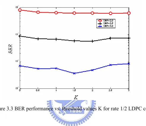
3.3 Proposed Dynamic Normalized-Offset-Compensation Technique for Min-Sum Algorithm...43
Chapter 4 Simulation Results and Analysis...45
4.1 Floating-Point Simulations ...46
4.2 Fixed-Point Simulations...50
5.1 The Whole Decoder Architecture ...52
5.2 Hardware Performance Comparison and Summary ...65
Chapter 6 Conclusions and Future Work...68
6.1 Conclusions...68
6.2 Future Work ...68
Appendix A: LDPC Codes Specification in IEEE 802.16e OFDMA...70
References ...73
List of Tables
Table 2.1 Efficient computation step of 1
(
1)
1
T T
p = −φ− −ET A C s− + ...15
Table 2.2 Efficient computation step of 1( 1 ) 2 T T T Bp As T p =− − + ...15
Table 2.3 Summary of Richardson’s encoding procedure. ...16
Table 2.4 Summary of sum-product algorithm...33
Table 2.5 Summary of min-sum algorithm...34
Table 5.1 Comparison of direct and backhanded CNU architectures...61
Table 5.2 Area, speed, and power consumption of the CNU using min-sum algorithm and modified min-sum algorithm ...66
List of Figures
Figure 2.1 Example of a (8, 4, 2)-regular LDPC code and its corresponding
Tanner graph. ...4
Figure 2.2 Example of an LDPC code matrix, where (n, r, c) = (20, 4, 3)...7
Figure 2.3 The parity-check matrix H of a block-LDPC code...9
Figure 2.4 Example of a rate-1/2 quasi-cyclic code from two circulant matrices, where a1(x)= 1+x and a2(x)=1+x2 +x4 ...10
Figure 2.5 The parity-check matrix in an approximate lower triangular form...13
Figure 2.6 (a) Example of a rate-1/2 quasi-cyclic code. (a) Parity-check matrix with two circulants, where a1(x)= 1+x and a2(x)=1+x2 +x4...18
Figure 2.6 (b) Example of a rate-1/2 quasi-cyclic code. (b) Corresponding generator matrix in systematic form ...18
Figure 2.7 Tanner graph of the given example parity-check matrix. ...25
Figure 2.8 Serial configuration for check node update function...29
Figure 2.9 Check node update function of sum-product algorithm ...30
Figure 2.10 Check node update function of min-sum algorithm ...30
Figure 2.11 Notations for iterative decoding procedure...31
Figure 2.12 The whole LDPC decoding procedure...33
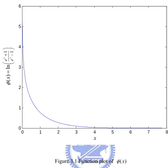
Figure 3.1 Function plot of φ( )x ...37
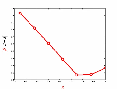
Figure 3.2 The absolute difference between the normalization technique and sum-product algorithm, vs. the of normalization factor β ...42
Figure 3.3 BER performance vs. threshold values K for rate 1/2 LDPC code...44
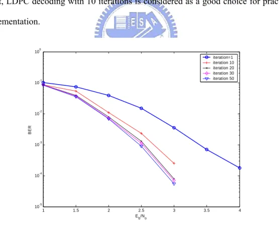
Figure 4.1 Decoding performance at different iteration numbers ...46
Figure 4.2 BER performance of the rate-1/2 code at different codeword lengths, in AWGN channel, maximum iteration=10 ...47
Figure 4.3 Floating-point BER simulations of two decoding algorithms in AWGN channel with code length=576, code rate=1/2, maximum iteration=10
...47
Figure 4.4 Floating-point BER simulations of normalized min-sum decoding algorithms in AWGN channel with code length=576, code rate=1/2, maximum iteration=10...48
Figure 4.5 Floating-point BER simulations under normalized-offset technique in min-sum decoding algorithms, in AWGN channel with code length=576, code rate=1/2, maximum iteration=10...48
Figure 4.6 Floating-point BER simulations of the dynamic normalized-offset min-sum decoding algorithm and its comparison with other algorithms, in AWGN channel with code length=576, code rate=1/2, maximum iteration=10...49
Figure 4.7 Floating-point BER simulations under normalized-offset compensated technique and dynamic normalization technique in min-sum algorithm. ...49
Figure 4.8 Fixed-point BER simulations of three different quantization configurations of min-sum decoding algorithm, in AWGN channel, code length=576, code rate=1/2, maximum iteration=10 ...50
Figure 4.9 Floating-point vs. fixed-point BER simulations of the normalization and dynamic normalized-offset min-sum algorithm...51
Figure 5.1 The parity-check matrix H of block-LDPC code...52
Figure 5.2 The partition of parity-check matrix H ...53
Figure 5.3 I/O pin of the decoder IP...53
Figure 5.5 A simple parity-check matrix example, based on shifted identity matrix
...55
Figure 5.6(a) The sub-modules of the whole decoder ...55
Figure 5.6(b) The outputs of the module INDEX...56
Figure 5.7(a) Values shuffling before sending to check node updating unit ...56
Figure 5.7(b) Values shuffling before sending to bit node updating unit ...57
Figure 5.8(a) The architecture of CNU using min-sum algorithm ...58
Figure 5.8(b) The architecture of CNU using modified min-sum algorithm...58
Figure 5.9 Block diagram of CS6 module...59
Figure 5.10(a) Block diagram of CMP-4 module...60
Figure 5.10(b) Block diagram of CMP-6 module...60
Figure 5.11 CNU architecture using min-sum algorithm...61
Figure 5.12 The architecture of the bit node updating unit with 4 inputs ...62
Figure 5.13(a) The architecture of RE-4B based MMU...63
Figure 5.13(b) The timing diagram of the message memory units...64
Figure 5.14 The message passing snapshots between MMU0 and MMU1 ...65
Figure A.1 Base matrix of the rate 1/2 code ...71
Figure A.2 Base matrix of the rate 2/3, type A code ...71
Figure A.3 Base matrix of the rate 2/3, type B code...72
Figure A.4 Base matrix of the rate 3/4, type A code ...72
Figure A.5 Base matrix of the rate 3/4, type B code...72
Chapter 1
Introduction
1.1 Background of LDPC Codes
Low-density parity check (LDPC) code, a linear block code defined by a very sparse parity-check matrix, was first introduced by Gallager [1]. Due to the difficulty in circuit implementation, LDPC codes have been ignored for about forty years except for the study of codes defined on graphs by Tanner [3]. The rediscovery of LDPC code was done by MacKay [10]. It has engaged much research interest ever since, because the sparse property of parity-check matrix makes the decoding algorithm simple and practical with good communication throughput rates. LDPC code is currently widely considered a serious competitor to the turbo codes. The main advantages of LDPC codes over turbo codes are that LDPC decoders are known to require an order of magnitude less arithmetic computations, and the decoding algorithms for LDPC codes are parallelizable and can potentially be accomplished at significantly greater speeds. The main decoding algorithm of LDPC codes is sum-product algorithm [10]. However, sum-product algorithm is prone to quantization errors while realized in hardware. Thus, several reduced-complexity algorithms with different levels of performance degradation have been proposed [14]. The thesis proposed a dynamically normalized-offset technique to improve the decoding performance and reduce the decoding complexity.
The implementation of LDPC codes decoders can be classified into fully parallel decoders, and partial-parallel decoders. The fully parallel decoders directly map the corresponding bipartite graph [17] into hardware and all the processing units are hard-wired according to the connectivity of the graph. Thus they can achieve very high decoding speed but have a high hardware cost. Another approach is to have a partial-parallel decoder [19], in which the functional units are reused in order to decrease the chip-area. Moreover, this architecture can process two different codewords concurrently to has moderate throughput. The other aim of this thesis is to improve the partial-parallel architecture and save chip area, with little degradation of the throughput.
1.2 Thesis Organization
This thesis is organized as follows. In chapter 2, basic concept of the LDPC codes: the code construction, encoding concept and various decoding algorithms will be introduced. Chapter 3 will first introduce the modified min-sum algorithm which uses the normalized technique. Then we propose a new dynamic normalized-offset technique for min-sum decoding algorithm. In chapter 4, the simulation results for the LDPC code which is discussed in chapter 2 and chapter 3 will be shown. In chapter 5, hardware architecture of the LDPC decoder will be discussed here. In the end of this thesis, brief conclusions and future work will be presented in chapter 6.
Chapter 2
Low-Density Parity-Check Codes
In this chapter, an introduction to low-density parity-check code will be given, including the fundamental concepts of LDPC code, code construction, encoding mechanism and decoding algorithm.
2.1 Fundamental Concept of LDPC Code
A binary LDPC code is a binary linear block code that can be defined by a sparse binary m×n parity-check matrix. A matrix is called a sparse matrix because there is
only a small fraction of its entries are ones. In other words, most part of the parity-check matrix are zeros and the else part of that are ones.
For any m×n parity-check matrix H, it defines a (n, k, r, c)-regular LDPC code
if every column vector of H has the same weight c and every row vector of H has the same weight r. Here the weight of a vector is the number of ones in the vector.
k= −n m. By counting the ones in H, it follows that n c× = ×k r. Hence if m<n,
then c<r. Suppose the parity-check matrix has full rank, the code rate of H is
(r−c) /r= −1 c r/ . If all the column-weights or the row-weights are not the same, an LDPC code is said to be irregular.
As suggested by Tanner [7], an LDPC code can be represented by a bipartite graph. An LDPC code corresponds to a unique bipartite graph and a bipartite graph also corresponds to a unique LDPC code. In a bipartite graph, one type of nodes, called the variable (bit) nodes, correspond to the symbols in a codeword. The other type of nodes, called the check nodes, correspond to the set of parity check equations. If the parity-check matrix H is an m×n matrix, it has m check nodes and n variable
nodes. A variable node vi is connected to a check node cj by an edge, denoted as (vi, cj),
if and only if the entry hi,j of H is one. A cycle in a graph of nodes and edges is
defined as a sequence of connected edges which starts from a node and ends at the same node, and satisfies the condition that no node (except the initial and final node) appears more than one time. The number of edges on a cycle is called the length of the cycle. The length of the shortest cycle in a Tanner graph is called the girth of the graph.
Regular LDPC codes are those where all nodes of the same type have the same degree. The degree of a node is the number of edges connected to that node. For example, Figure2.1 shows a (8, 4, 4, 2)-regular LDPC code and its corresponding
3 c 1 c c2 c4 1 v v2 v3 v4 v5 v6 v7 v8
nodes
check
nodes
variable
3 c 1 c c2 c4 1 v v2 v3 v4 v5 v6 v7 v8nodes
check
nodes
variable
Figure 2.1 (8, 4, 4, 2)-regular LDPC code and its corresponding Tanner graph.
⎥
⎥
⎥
⎥
⎦
⎤
⎢
⎢
⎢
⎢
⎣
⎡
=
1
0
0
1
1
0
1
0
0
1
1
0
0
1
1
0
1
0
1
0
1
0
0
1
0
1
0
1
0
1
0
1
H
Tanner graph. In this example, there are 8 variable nodes (vi), 4 check nodes (ci), the
row weight is 4 and the column weight is 2. The edges (c1, v3), (v3, c3), (c3, v7), and (v7,
c1) depict a cycle in the Tanner graph. Since this turns out to be the shortest cycle, the
girth of the Tanner graph is 4. Irregular LDPC codes were introduced in [8] and [9].
2.2 Constructions of LDPC Codes
This section is going to discuss the parity-check matrix H of LDPC code. The design of H is the moment when the asymptotical constraints (the parameters of the class you designed, like the degree distribution, the rate) have to meet the practical constraints (finite dimension, girths).
Here, we describe some recipes which take some practical constraints into account. Two techniques exist in the literature: random and deterministic ones. The design compromise is that for increasing the girth, the sparseness has to be decreased, so is the code performance decreased due to a low minimum distance. On the contrary, for high minimum distance, the sparseness has to be increased yielding the creation of low-length girth, due to the fact that H dimensions are finite, and thus, yielding a poor convergence of sum-product algorithm.
2.2.1 Random Code Construction
The first constructions of LDPC codes are random ones. They were proposed by
Gallager [1] and MacKay [10]. The parity check matrix in Gallager’s method is a
concatenation and/or superposition of sub-matrices; these sub-matrices are created by performing some permutations on a particular (random or not) sub-matrix which usually has a column weight of 1. The parity check matrix in MacKay’s method is computer-generated. These two methods are introduced below.
Gallager’s method [1]
Define an (n, r, c) parity check-matrix as a matrix of n columns that has c ones in each column, r ones in each row, and zeros elsewhere. Following this definition, an (n,
r, c) parity-check matrix has nc r/ rows and thus a rate of coderate≥ −1 c r/ . In
order to construct an ensemble of (n, r, c) matrices, consider first the special (n, r, c) matrix in Figure 2.2, where n, r and c are 20, 4 and 3, respectively.
1 0 0 0 0 1 0 0 0 0 1 0 0 0 0 1 0 0 0 0 0 0 0 1 0 0 1 0 0 0 0 1 0 0 0 0 1 0 0 0 0 1 0 0 0 0 0 1 0 0 0 0 1 0 0 0 0 1 0 0 0 0 0 0 1 0 0 0 0 1 0 0 0 1 0 0 0 0 1 0 0 0 1 0 0 0 0 0 1 0 0 0 0 0 1 0 0 0 0 1 1 0 0 0 1 0 0 0 1 0 0 0 1 0 0 0 0 0 0 0 0 1 0 0 0 1 0 0 0 1 0 0 0 0 0 0 1 0 0 0 0 0 1 0 0 0 1 0 0 0 0 0 0 1 0 0 0 1 0 0 0 0 0 1 0 0 0 0 0 0 1 0 0 0 1 0 0 0 1 0 0 0 0 0 0 0 0 1 0 0 0 1 0 0 0 1 0 0 0 1 1 1 1 1 0 0 0 0 0 0 0 0 0 0 0 0 0 0 0 0 0 0 0 0 1 1 1 1 0 0 0 0 0 0 0 0 0 0 0 0 0 0 0 0 0 0 0 0 1 1 1 1 0 0 0 0 0 0 0 0 0 0 0 0 0 0 0 0 0 0 0 0 1 1 1 1 0 0 0 0 0 0 0 0 0 0 0 0 0 0 0 0 0 0 0 0 1 1 1 1
Figure 2.2 Example of an LDPC code matrix, where (n, r, c)=(20,4,3)
This matrix is divided into c sub-matrices, each containing a single 1 in each column. The first of these sub-matrices contains all its 1’s in descending order where the ith row contains 1’s in columns ( 1)i− r+ to ir . The other sub-matrices are 1 merely column permutations of the first. We define the ensemble of (n, r, c) codes as the ensemble resulting from random permutations of the columns of each of the bottom (c− sub-matrices of a matrix such as in Figure 2.2 with equal probability 1) assigned to each permutation. This definition is somewhat arbitrary and is made for mathematical convenience. In fact such an ensemble does not include all (n, r, c) codes as just defined. Also, at least (c− rows in each matrix of the ensemble are 1) linearly dependent. This simply means that the codes have a slightly higher information rate than the matrix indicates.
MacKay’s method [10]
A computer-generated code was introduced by MacKay [10]. The parity-check matrix is randomly generated. First, parameters n, m, r, and c are chosen to conform an (n, m, r, c)-regular LDPC code where n, r and c are the same as in Gallager’s code and m is the number of the parity-check equations in H. Then, 1’s are randomly generated into c different positions of the first column. The second column is generated in the same way, but checks are made to insure that no two columns have a 1 in the same position more than twice in order to avoid 4-cycle in the Tanner graph. If there is a 4-cycyle in the Tanner graph, the decoding performance will be reduced by about 0.5dB. Avoidance of 4-cycles in a parity-check matrix is therefore required. The next few columns are generated sequentially and checks for 4-cycles must be performed in each generation. In this procedure, the number of 1’s in each row must be recorded, and if any row already has r ones, the next-column generation will not select that row.
2.2.2 Deterministic Code Construction
A parity-check matrix H by random construction is sparse, but its corresponding generator matrix is not. This property will increase encoding complexity. To circumvent this problem, deterministic code construction schemes have been proposed. It can lead to low encoding complexities. Some forms of the deterministic code construction include block-LDPC code, quasi-cyclic code [5], and quasi-cyclic based code [21]. They are introduced below.
Block-LDPC Code
The parity check matrix H based on block-LDPC code is composed by several sub-matrices. The size of H is m-by-n. The sub-matrices are shifted identity matrices or zero matrices. The matrix form of H is shown in Figure 2.3. Sub-matrix P is i j,
one of a set of z-by-z permutation matrices or a z-by-z zero matrix. Matrix H is expanded from a binary base matrix H of size b m -by-b n , where b m= ⋅z mb ,
b
n= ⋅ , and z is an integer ≥ 1. The base matrix is expanded by replacing each 1 z n
in the base matrix with a z-by-z permutation matrix, and each 0 with a z-by-z zero matrix. The used permutations are circular right shifts, and the set of permutation matrices contains the z-by-z identity matrix and circularly right-shifted versions of the identity matrix. The details of block-LDPC Code can be seen in Appendix A.
0,0 0,1 0, 1 1,0 1,1 1, 1 1,0 1,1 1, 1 b b b b b b n n m m m n P P P P P P H P P P − − − − − − ⎡ ⎤ ⎢ ⎥ ⎢ ⎥ = ⎢ ⎥ ⎢ ⎥ ⎢ ⎥ ⎣ ⎦ L L M M L M L
Figure 2.3 The parity-check matrix H of a block-LDPC code
Quasi-Cyclic Code [5]
A code is quasi-cyclic if, for any cyclic shift of a codeword by l places, the
resulting word is also a codeword. A cyclic code is a quasi-cyclic code with l=1. Consider the binary quasi-cyclic codes described by a parity-check matrix
] ,... ,
[A1 A2 Al
H = (2.10)
where A1,A2,...Al are binary v×v circulant matrices. The algebra of
(
v×v)
binary circulant matrices is isomorphic to the algebra of polynomials modulo v−1
over GF(2). A circulant matrix A is completely characterized by the polynomial 1 1 2 2 1 0 .... ) ( = + + + + − v− v x a x a x a a x a (2.11)
where the coefficients are from the first row of A , and a code C with parity-check matrix of the form (2.10) can be completely characterized by the polynomials
) ( ),..., ( ), ( 2 1 x a x a x
a l . Figure 2.4(a) shows an example of a rate-1/2 quasi-cyclic
code, where a1(x)= 1+x and a2(x)=1+x2 +x4 . Figure 2.4(b) shows the
corresponding Tanner graph representation. For this example, we can see the edges (c1, v6), (v6, c4), (c4, v8), (v8, c1) depict a 4-cycle in this graph which is to be avoided
for performance consideration.
⎥ ⎥ ⎥ ⎥ ⎥ ⎥ ⎦ ⎤ ⎢ ⎢ ⎢ ⎢ ⎢ ⎢ ⎣ ⎡ = 1 1 0 1 0 0 1 1 0 1 1 0 1 1 0 0 1 0 1 1 1 0 1 0 1 1 0 0 0 1 1 1 0 0 0 0 1 1 0 0 0 0 1 1 0 0 0 0 1 1 H
(a) A parity-check matrix with two circulant matrices
3
c
1c
c
2c
4 1v
v
2v
3v
4v
5v
6v
7v
8nodes
check
nodes
variable
5c
9v
v
10 3c
1c
c
2c
4 1v
v
2v
3v
4v
5v
6v
7v
8nodes
check
nodes
variable
5c
9v
v
10(b) Tanner graph representation
Figure2.4 Example of a rate-1/2 quasi-cyclic code from two circulant matrices, where
x x
Quasi-Cyclic Based Code [21]
The code is constructed with a base of quasi-cyclic code. The parity check matrix is in the following form.
⎥ ⎦ ⎤ ⎢ ⎣ ⎡ = − − l l l B B B B A A A H 1 2 1 1 2 1 ... 0 ... (2.12) where A1,A2,...,Al−1,B1,B2,...,andBl are all v×v circulant matrices. The code
length is vl and the code rate is ( l
2
1− ). We can use the difference families [21] to determine the polynomials of each of the circulant matrix ai(x) and bj(x), where
} 1 ,..., 2 , 1 { − ∈ l
i and j∈{1,2,...,l}, just as the quasi-cyclic code. In order to avoid
any 4-cycles in the new structure of the parity-check matrix, we provide a new difference family to solve this problem. First, construct two (v,γ,1) difference families Family A and Family B and combine the two families to form a new difference Family C , subject to the following two constraints.
Constraint 1: The differences [(ai,x −ai,y) mod v] and [(bi,x −bi,y) mod v],
where i=1,2,...,l−1 ;x,y=1,2,...,γ ,x≠ y, give each element, can not be the same.
Constraint 2: The differences [(ai,x −aj,y) mod v] and [(bi,x−bj,y) mod v],
where , i, j=1,2,...,l−1,i≠ j ;x,y=1,2,...,γ give each element, can not be the same.
2.3 Encoding of LDPC Codes
Since LDPC code is a linear block code, it can be encoded by conventional methods. However, conventional methods require encoding complexities proportional to the quadratic of the code length. The high encoding cost of LDPC code becomes a major drawback when compared to the turbo codes which have linear time encoding
complexity. In this section, we will introduce some improved methods.
2.3.1 Conventional Method
Let ]u=[u0,u1,u2,...,uk−1 be a row vector of message bits with length k and
] ,..., , , [ 0 1 2 −1 = c c c cn
c be a codeword with length n. Let G with dimension k n× be
the generating matrix of this code, and
uG
c= . (2.12)
If H is the parity-check matrix of this code with dimension m n× , where m= −n k,
then 0 0 0 0 = ⇒ = ⇒ = ⇒ = T T T T T GH uGH cH Hc (2.13)
Suppose a sparse parity-check matrix H with full rank is constructed. Gaussian elimination and column reordering can be used to derive an equivalent parity-check matrix in the systematic form Hsystematic =[PIr]. Thus equation (2.13) can be solved to get the generating matrix in a systematic form as
]
[ T
k systematic I P
G = . (2.14)
Finally, the generating matrix G can be obtained by doing the reverse column reordering to the Gsystematic.
Triangularized parity-check matrix form [4]
In [4], it suggests to force the parity-check matrix to be in a lower triangular form. Under this restriction, it guarantees a linear time encoding complexity, but, in
general, it also results in some loss of performance.
2.3.2 Richardson’s Method [3]
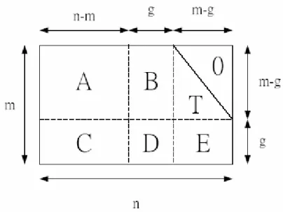
Richardson’s method is the most extensively used among LDPC encoding algorithms. Figure 2.5 shows how to bring a parity-check matrix into an approximate lower triangular form using row and column permutations. Note that since this
Figure 2.5 The parity-check matrix in an approximate lower triangular form transformation was accomplished solely by permutations, the parity check matrix H is still sparse. This method is to cut the parity check matrix H into 6 sub-matrices: A, B,
T, C, D, E. Especially, the sub-matrix T is in lower triangular form.
More precisely, it is assumed that the matrix is written in the form ⎟⎟ ⎠ ⎞ ⎜⎜ ⎝ ⎛ = E D C T B A H (2.15) where A is (m−g)×(n−m), B is (m− )g ×g , T is (m−g)×(m−g), C is ) (n m
g× − , D is g× , and E is g g×(m−g). Further, all these matrices are sparse
codeword of this parity-check matrix where s is the message bits with length
)
(m− , n p1 combined with p2 are the parity bits, and p1 and p2 have length g , and (m−g), respectively. Multiplying the matrix in equation (2.16) on both sides
of the constraint equation T 0
H x⋅ = ⎟⎟ ⎠ ⎞ ⎜⎜ ⎝ ⎛ − − I ET I 1 0 (2.16) can result in 1 1 0 0 T A B T x ET A C− ET B− D ⎛ ⎞ ⋅ = ⎜− + − + ⎟ ⎝ ⎠ . (2.17)
Expanding equation (2.17), one can get equations (2.18) and (2.19) 0 2 1 + = + T T T Tp Bp As (2.18)
(
− −1 +) (
T + − −1 +)
1T =0 p D B ET s C A ET . (2.19) Define 1 ET B Dφ = − − + and assume for the moment that φ is nonsingular. Then
from equation (2.19) we conclude that
(
)
1 1 1
T T
p = −φ− −ET A C s− + . (2.20)
Hence, once the g×(n−m) matrix −φ−1
(
−ET A C s−1 +)
T has been pre-computed,the determination of p1 can be accomplished with a time complexity of
( ( ))
O g× −n m simply by performing a multiplication with this (generally dense)
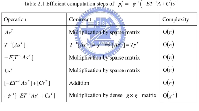
matrix. This complexity can be further reduced as shown in Table 2.1. Rather than
pre-computing 1
(
1)
TET A C s
φ− −
− − + and then multiplying with T
s , p1 can be
determined by breaking the computation into several smaller steps, each of which is computationally efficient. To this end, we first determine T
As , which has complexity
of ( )O n , because A is sparse. Next, we multiply the result by T−1. Since
T T
y As
T−1[ ]= is equivalent to the system [AsT]=TyT , this can also be
accomplished in ( )O n time by back-substitution method, because T is lower
the overall complexity of determining p1 is O n( +g2). In a similar manner, noting
from equation (2.18) that 1( 1 )
2 T T T Bp As T
p =− − + , we can determine p2 in time
complexity of O n , as shown step by step in Table 2.2. ( )
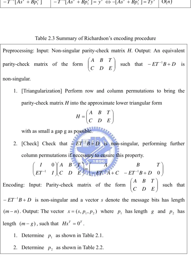
A summary of this efficient encoding procedure is given in Table 2.3. It contains two steps, the preprocessing step and the actual encoding step. In the preprocessing step, we first perform row and column permutations to bring the parity-check matrix into the approximate lower triangular form with as small a gap g as possible. In actual encoding, it contains the steps listed in Table 2.1 and 2.2. The overall encoding
complexity is ( 2)
O n+g , where g is the gap of the approximate triangularization.
Table 2.1 Efficient computation steps of 1
(
1)
1
T T
p = −φ− −ET A C s− +
Operation Comment Complexity
T As ] [ 1 T As T− ] [ 1 T As T E − − T Cs ] [ ] [ 1 T T Cs As ET + − − 1[ 1 T T] ET As Cs φ− − − − +
Multiplication by sparse matrix
T T T T Ty As y As T−1[ ]= ⇔[ ]=
Multiplication by sparse matrix Multiplication by sparse matrix Addition
Multiplication by dense g× matrixg
( )
n Ο( )
n Ο( )
n Ο( )
n Ο( )
n Ο( )
2 g ΟTable 2.2 Efficient computation steps of 1( 1 )
2 T T T Bp As T p =− − +
Operation Comment Complexity
T As T Bp1 ] [ ] [ T 1T Bp As +
Multiplication by sparse matrix Multiplication by sparse matrix Addition
( )
n Ο( )
n Ο( )
n Ο] [ 1 1 T T Bp As T + − − T T T T T T Ty Bp As y Bp As T + = ⇔− + = − − [ ] [ ] 1 1 1 Ο
( )
nTable 2.3 Summary of Richardson’s encoding procedure
Preprocessing: Input: Non-singular parity-check matrix H. Output: An equivalent
parity-check matrix of the form ⎟⎟
⎠ ⎞ ⎜⎜ ⎝ ⎛ E D C T B A such that −ET−1B+D is non-singular.
1. [Triangularization] Perform row and column permutations to bring the parity-check matrix H into the approximate lower triangular form
⎟⎟ ⎠ ⎞ ⎜⎜ ⎝ ⎛ = E D C T B A H
with as small a gap g as possible.
2. [Check] Check that −ET−1B+D is non-singular, performing further
column permutations if necessary to ensure this property.
⎟⎟ ⎠ ⎞ ⎜⎜ ⎝ ⎛ + − + − = ⎟⎟ ⎠ ⎞ ⎜⎜ ⎝ ⎛ ⎟⎟ ⎠ ⎞ ⎜⎜ ⎝ ⎛ − − − 0 0 1 1 1 D B ET C A ET T B A E D C T B A I ET I
Encoding: Input: Parity-check matrix of the form ⎟⎟
⎠ ⎞ ⎜⎜ ⎝ ⎛ E D C T B A such that D B ET +
− −1 is non-singular and a vector s denote the message bits has length
)
(m− . Output: The vector n x=(s,p1,p2) where p1 has length g and p2 has
length )(m−g , such that HxT =0T.
1. Determine p1 as shown in Table 2.1.
2.3.3 Quasi-Cyclic Code [5]
As reviewed in section 2.2, the quasi-cyclic code can be described by a parity-check matrix H =[A1,A2,...Al] and each of a circulant matrix A is j
completely formed by the polynomial 1
1 1 0 .... ) ( = + + + − v− v x a x a a x a with
coefficients from its first row. A code C with parity-check matrix H can be completely characterized by the polynomials a x1( ), ( ),..., a x2 and ( )a x . As for the encoding, if l
one of the circulant matrices is invertible (say A ) the generator matrix for the code l
can be constructed in the following systematic form.
⎥ ⎥ ⎥ ⎥ ⎥ ⎦ ⎤ ⎢ ⎢ ⎢ ⎢ ⎢ ⎣ ⎡ = − − − − − T l l T l T l l v A A A A A A I G ) ( ... ) ( ) ( 1 1 2 1 1 1 ) 1 ( (2.21)
It results in a quasi-cyclic code of length vl and dimension v(l−1). The encoding
process can be achieved with linear complexity using a v(l−1)-stage shift register. Regarding the algebraic computation, the polynomial transpose is defined as
∑
− = − = 1 0 , ) ( n i i n i T x a x a xn =1. (2.22)For a binary [n, k] code, length n=vl and dimension k = lv( −1), the k-bit message
[
i0,i1,...,ik−1]
is described by the polynomial1 1 1 0 ... ) ( = + + + − k− k x i x i i x i and the
codeword for this message is c(x)=[i(x),xkp(x)], where p(x) is given by
, )) ( ) ( ( ) ( ) ( 1 1 1
∑
− = − ∗ ∗ = l j T j l j x a x a x i x p (2.23)where )ij(x is the polynomial representation of the information bits iv(j−1) to ivj−1,
1 1 1 ) 1 ( ) 1 ( ... ) ( − − + − − + + + = v vj j v j v j x i i x i x i (2.24)
and polynomial multiplication (∗ is mod ) v −1
As an example, consider a rate-1/2 quasi-cyclic code with v=5, l =2, the first
circulant is described by a1(x)= 1+x and the second circulant is described by
4 2 2(x) 1 x x
a = + + , which is invertible and
4 2
1
2 (x) x x x
a − = + + . (2.25)
The generator matrix contains a 5×5 identity matrix and the 5×5 matrix
described by the polynomial
3 2 1 1 2 ( ) ( )) (1 ) 1 (a− x ∗a x T = +x T = +x . (2.26)
Figure 2.6 shows the example parity-check matrix and the corresponding generator matrix. ⎥ ⎥ ⎥ ⎥ ⎥ ⎥ ⎦ ⎤ ⎢ ⎢ ⎢ ⎢ ⎢ ⎢ ⎣ ⎡ = 1 1 0 1 0 0 1 1 0 1 1 0 1 1 0 0 1 0 1 1 1 0 1 0 1 1 0 0 0 1 1 1 0 0 0 0 1 1 0 0 0 0 1 1 0 0 0 0 1 1 H
(a) A parity-check matrix with two circulants
⎥ ⎥ ⎥ ⎥ ⎥ ⎥ ⎦ ⎤ ⎢ ⎢ ⎢ ⎢ ⎢ ⎢ ⎣ ⎡ = 1 0 1 0 0 0 1 0 1 0 0 0 1 0 1 1 0 0 1 0 0 1 0 0 1 1 0 0 0 0 0 1 0 0 0 0 0 1 0 0 0 0 0 1 0 0 0 0 0 1 G
(b) The corresponding generator matrix in systematic form
Figure 2.6 Example of a rate-1/2 quasi-cyclic code. (a) Parity-check matrix with two circulants, where a1(x)= 1+x and a2(x)=1+x2 +x4. (b) Corresponding generator
Quasi-Cyclic Based Code [21]
As reviewed in section 2.2, the quasi-cyclic based code can be described by a
parity-check matrix ⎥ ⎦ ⎤ ⎢ ⎣ ⎡ = − − l l l B B B B A A A H 1 2 1 1 2 1 ... 0 ... , where l l B B B A A
A1, 2,..., −1, 1, 2,...,and are all v×v circulant matrices. Regarding the
encoding for the quasi-cyclic based structure, suppose that two of the circulant matrices Al−1 and B are invertible, we can derive two generator matrices in the l
following systematic forms
[
( 2) 1]
2 1 1 2 1 1 1 1 1 ) 2 ( 1 ) ( ... ) ( ) ( G I A A A A A A I G v l T l l T l T l l v systematic − − − − − − − − − = ⎥ ⎥ ⎥ ⎥ ⎥ ⎦ ⎤ ⎢ ⎢ ⎢ ⎢ ⎢ ⎣ ⎡ = (2.27) and[
( 1) 2]
1 1 2 1 1 1 ) 1 ( 2 ) ( ... ) ( ) ( G I B B B B B B I G v l T l l T l T l l v systematic − − − − − − = ⎥ ⎥ ⎥ ⎥ ⎥ ⎦ ⎤ ⎢ ⎢ ⎢ ⎢ ⎢ ⎣ ⎡ = . (2.28)Let c=[d, p1,p2] denote the codeword of the proposed parity-check matrix where d is the message bits with length v(l −2), and p1 combined with p2 are the parity
bits, each having the same length v. The encoding procedure is partitioned into two
steps.
Encoding Step 1: We can use the generator matrix G1 to get the parity bits p1. That
is
1 1 d G
p = × . (2.29)
Then, combine the parity bits p1 with the message bits d to form an intermediate
Encoding Step 2: The last parity bits p2 can be derived from the generator matrix
2
G and the intermediate codeword c′. That is
p2 =c′×G2. (2.30)
2.4 Conventional LDPC Code Decoding Algorithm
There are several decoding algorithms for LDPC codes. The LDPC decoding algorithms can be summarized as: bit-flipping algorithm [20], and message passing algorithm [11]. In the following, we will make an introduction of the decoding algorithms.
2.4.1 Bit-Flipping Algorithm [20]
The idea for decoding is the fact that in case of low-density parity-check matrices the syndrome weight increases with the number of errors in average until errors weights are much larger than half the minimum distance. Therefore, the idea is to flip one bit in each iteration, and the bit to be flipped is chosen such that the syndrome weight decreases. It should be noted that not only rows of the parity-check matrix can be used for decoding, but in principle all vectors of the dual code with minimum (or small) weight. In the following, we will introduce two of the bit-flipping algorithms [20].
Notation and Basic Definitions
The idea behind this algorithm is to “flip” the least number of bits until the parity
check equation T 0
H x⋅ = is satisfied.Suppose a binary (n,k) LDPC code is used for
error control over a binary-input additive white Gaussian noise (BIAWGN) channel with zero mean and power spectral density σ2. The letter n is the code length and k
is the message length. Assume binary phase-shift-keying (BPSK) signaling with unit
energy is adopted. A codeword ( , , ,0 1 1) { (2)}n
n
c= c c L c− ∈ GF is mapped into bipolar
sequence x=( , , ,x x0 1 L xn−1) before its transmission, where xi = ⋅2 (ci − 1),
0≤ ≤ −i n 1. Let y=( , , ,y y0 1 L yn−1)be the soft-decision received sequence at the
output of the receiver matched filter. For 0≤ ≤ −i n 1, yi = + , where xi ni n is a i
Gaussian random variable with zero mean and variance σ2. An initial binary hard
decision of the received sequence, (0) (0) (0) (0)
0 1 1 ( , , , n ) z = z z L z − , is determined as follows (0) 1, 0 0, 0 i i i y z y ≥ ⎧ = ⎨ ≤ ⎩ (2.31) For any tentative binary hard decision z made at the end of ach decoding iteration, we
can compute the syndrome vector as T.
s=H z⋅ One can define the log-likelihood
ratio (LLR) for ear channel output yi, 0≤ ≤ − : i n 1 ln ( 1| ) ( 0 | ) i i i i i p c y L p c y = = = (2.32) The absolute value of L , i Li , is called the reliability of the initial decision
(0)
i
z .
For any binary vector v=( , , ,v v0 1L vn−1), let wt(v) be the Hamming weight of v . Let
i
u be the n dimensional unit vector, i.e., a vector with “1” at the i-th position and “0”
Algorithm I
Step (1) Initialization: Set iteration counter k = 0. Calculate (0)
z andS(0) =wt H z( ⋅ (0)T).
Step (2) If ( )k 0
S = , then go to Step (8).
Step (3) k←k+1. If k>kmax, where kmax is the maximum number of iterations, go to
Step (9).
Step (4) For each i=0,1, ,L n−1, calculate Si( )k wt H[ (z(k 1) ui) ]T
− = ⋅ + Step (5) Find ( )k {0,1, , 1} j ∈ L n− with ( ) ( ) 0 arg(min ) k k i i n j S ≤ < = . Step (6) If ( )k (k 1) j = j − , then go to Step (9). Step (7) Calculate ( ) ( ) ( 1) k k k j z =z − +u and S( )k =wt H z( ⋅ ( )kT). Go to Step (2).
Step (8) Stop the decoding and return ( )k
z .
Step (9) Declare a decoding failure and return (k 1)
z − .
So the algorithm flips only one bit at each iteration and the bit to be flipped is chosen according to the fact that, in average, the weight of the syndrome increases with the weight of the error. Note that in some cases, the decoder can choose a wrong position j, and thus introduce a new error. But there is still a high likelihood that this new error will be corrected in some later step of the algorithm.
Algorithm II
Algorithm I can be modified, with almost no increase in complexity, to achieve better error performance, by including some kind of reliability information (or measure) of the received symbols. Many algorithms for decoding linear block codes
based on this reliability measure have been devised. Consider the received soft-decision sequencey=( , , ,y y0 1 L yn−1). For the AWGN channel, a simple measure of the reliability,L , of a received symbol i y is its magnitude, i yi . The larger the
magnitude yi is, the larger the reliability of the hard-decision digit z is. If the i
reliability of a received symbol y is high, we want to prevent the decoding i
algorithm from flipping this symbol, because the probability of this symbol being erroneous is less than the probability of this symbol being correct. This can be achieved by appropriately increasing the values S in the decoding algorithm. The i
solution is to increase the values of S by the following term: i Li . The larger value
of Li implies that the hard-decision z is more reliable. The steps of the soft i
version of the decoding algorithm are described in detail below:
Step (1) Initialization: Set iteration counter k = 0. Calculate (0)
z andS(0) =wt H z( ⋅ (0)T).
Step (2) If ( )k 0
S = , then go to Step (8).
Step (3) k←k+1. If k >kmax, go to Step (9).
Step (4) For each i=0,1, ,L n−1, calculate Si( )k =wt H[ ⋅(z(k−1)+ui) ]T + Li
Step (5) Find ( )k {0,1, , 1} j ∈ L n− with ( ) ( ) 0 arg(min ) k k i i n j S ≤ < = . Step (6) If ( )k (k 1) j = j − , then go to Step (9). Step (7) Calculate ( ) ( ) ( 1) k k k j z =z − +u and S( )k =wt H z( ⋅ ( )kT). Go to Step (2).
Step (8) Stop the decoding and return ( )k
z .
Step (9) Declare a decoding failure and return (k 1)
It is important to point out that, in both algorithms, though the maximum number of iteration is specified, the algorithms have an inherent stopping criterion. The decoding process stops either when a valid codeword is obtained (Step 2) or when the minimum syndrome weight at the kth iteration and the minimum syndrome weight at the (k-1)th iteration are found in the same position (Step 6).
The bit-flipping algorithm just corrects at most one error bit in one iteration. The codeword length of LDPC code is usually hundreds (or thousands) of bits. When the channel SNR (signal-to-noise ratio) is low, the decoding iteration number of the bit-flipping algorithm needs to be high to correct the erroneous bits. This will lower the throughput of the decoder. And according to Step (5), equation (2.33) is to find the minimal value of the n numbers. The value of n (codeword length) is usually large. The hardware complexity of equation (2.33) is high.
( ) ( ) 0 arg(min ) k k i i n j S ≤ < = (2.33)
2.4.2 Message Passing Algorithm [11]
Since the bit-flipping algorithm is hard to be implemented in hardware, the message passing algorithm is extensively used for LDPC decoding. The message passing algorithm is an iterative decoding process. Messages between variable nodes and check nodes are exchanged back and forth. The decoder expects that error will be corrected progressively by using this iterative message-passing algorithm. At present, there are two types of iterative decoding algorithms applied to LDPC codes in general.
Sum-product algorithm, also known as belief propagation algorithm. Min-sum algorithm
Both of sum-product algorithm and min-sum algorithm are message passing algorithms. In the following, we will discuss these two algorithms in detail. First, we explain the decoding procedure in Tanner graph below.
Decoding Procedure in Tanner Graph Form
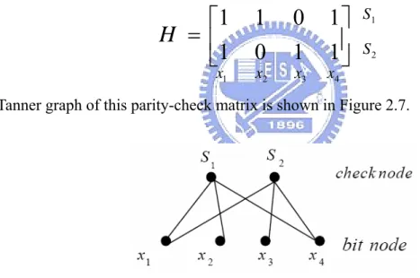
Now we make a description of the message passing algorithm using Tanner graph form. Here is a simple example of irregular LDPC code. The parity-check matrix is shown below.
Tanner graph of this parity-check matrix is shown in Figure 2.7.
Figure 2.7 Tanner graph of the given example parity-check matrix
Assume every line in the Tanner graph has two information messages. One is expressed in a solid line and the other is expressed in a dotted line. We use the messages to decode the received signal. For convenience of explanation, we take one part of Tanner graph which is shown below.
1 1
0 1
1 0
1 1
H
= ⎢
⎡
⎤
⎥
⎣
⎦
S2 1 x x2 x3 x4 1 SThe solid line and the dotted line are represented by qs→x and rx→s, respectively. In
this example, we can get qs1→x1 by rx2→s1 and rx4→s1. Equation (2.34) shows how to
compute qs1→x1.
1 1 ( 2 1 4 1)
s x x s x s
q → =CHK r → ⊕r → (2.34)
On the other hand, we can also get rx1→s1 by qs2→x1 and L , where 1 L is the 1
initialization value. The initialization value L will be discussed later. Equation (2.35) 1
shows how to compute
1 1 x s r → . 1 1 ( 2 1 1) x s s x r → =VAR q → ⊕L (2.35)
There is CHK function in equation (2.34) and VAR function in equation (2.35).
The two special functions will be introduced in the following contents. In the Tanner graph, we can compute the solid line message qs→x by the dotted line messages rx→s
dotted line message rx→s by the real line messages qs→x which are connected to the
same bit node. So the values of rx→s and qs→x are updated iteratively. We call this
iterative decoding.
Decoding Procedure in Matrix Form
Because Tanner graph is a representation of the parity-check matrix H, we can also use the matrix form to replace Tanner graph form. Let us take the same
parity-check matrix H in the previous section 1 1 0 1
1 0 1 1
H = ⎢⎡ ⎤⎥
⎣ ⎦ as an example. In
equation (2.36) and equation (2.37), we define matrix Q and matrix R. The positions of the nonzero values in R and Q are the same as those of the ones in H.
1 1 1 2 1 4 2 1 2 3 2 4 0 0 s x s x s x s x s x s x q q q Q q q q → → → → → → ⎡ ⎤ = ⎢ ⎥ ⎢ ⎥ ⎣ ⎦ (2.36) 1 1 2 1 4 1 1 2 3 2 4 2 0 0 x s x s x s x s x s x s r r r R r r r → → → → → → ⎡ ⎤ = ⎢ ⎥ ⎢ ⎥ ⎣ ⎦ (2.37)
The elements in the matrix Q are computed by the elements in the matrix R, for example, qs1→x1 =CHK r( x2→s1⊕rx4→s1). On the other hand, the elements in the matrix
R are computed by the elements in the matrix Q. For example,
1 1 ( 2 1 1)
x s s x
r → =VAR q → ⊕L , where L is the initialization value. So the elements in 1
matrix R and Q are updated iteratively. We can also regard the CHK function as the
In the LDPC iterative decoding procedure, there are two main functions: VAR
and CHK. Equation (2.38) shows the VAR function with two inputs and equation
(2.39) is the general form of the VAR function.
1 2 1 2 ( ) VAR q ⊕q = + q q (2.38) 1 2 1 2 ( l) l VAR q ⊕ ⊕ ⊕q L q = +q q + +L q (2.39)
The VAR function is fixed regardless of the decoding algorithms. It is just a
summation operation.
The CHK function with two inputs can be reformulated in different forms.
There are )) ( ) ( ( ) ( ) ( )) 2 tanh( ) 2 (tanh( tanh 2 ) ( 2 1 2 1 2 1 1 2 1 L L L sign L sign L L L L CHK φ φ φ + = × = ⊕ − (2.40) where ⎟⎟ ⎠ ⎞ ⎜⎜ ⎝ ⎛ − + = ⎟⎟ ⎠ ⎞ ⎜⎜ ⎝ ⎛ ⎟ ⎠ ⎞ ⎜ ⎝ ⎛ − = 1 1 ln 2 tanh ln ) ( x x e e x x φ and φ(φ(x))=x, (2.41) and 2 1 2 1 1 1 ln 2 2 )) 2 ln(cosh( )) 2 ln(cosh( ) ( 2 1 2 1 2 1 2 1 2 1 L L L L e e L L L L L L L L L L CHK − − + − + + + − − + = − − + = ⊕ 2 1 2 1 1 1 ln ) , min( ) sign(L ) sign(L1 2 1 2 L L L L e e L L − − + − + + + × × = (2.42)
≈sign(L1)×sign(L2)×min(L1, L2). (2.43) When CHK function is in the form of equation (2.40) or equation (2.42), we call the
decoding algorithm as sum-product algorithm. The fourth term
2 1 2 1 1 1 ln L L L L e e − − + − + + in equation (2.42) is called the correction factor. When the check node computation is in
the form of equation (2.43), or in other words an approximate form, we call it the min-sum algorithm.
The above discussion of check node computation is only about the CHK
function with two inputs. Now, we will discuss the general form of the CHK
function. The general form of the CHK function can be expressed in equation
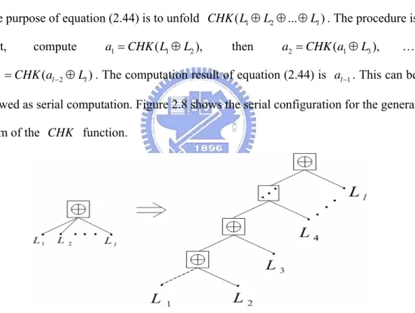
(2.44). ) )...) ) ( ( (... ( ) ... (L1 L2 Ll CHK CHK CHK CHK L1 L2 L3 Ll CHK ⊕ ⊕ ⊕ = ⊕ ⊕ ⊕ (2.44)
The purpose of equation (2.44) is to unfold CHK L( 1⊕L2⊕ ⊕... Ll). The procedure is:
first, compute a1=CHK L( 1⊕L2), then a2 =CHK a( 1⊕L3), …,
1 ( 2 )
l l l
a− =CHK a− ⊕L . The computation result of equation (2.44) is al−1. This can be
viewed as serial computation. Figure 2.8 shows the serial configuration for the general
form of the CHK function.
Figure 2.8 Serial configuration for check node update function
The serial computation has a long critical path in the check node update unit.
From equations (2.40), (2.43), and (2.44), we can generalize the CHK function as
equation (2.45) for sum-product algorithm, and equation (2.46) for min-sum algorithm.
1 2 1 2 1 ( l) l ( ) [ (i ) ( ) ( l)] i CHK L L L sign L φ φ L φ L φ L = ⊕ ⊕ ⊕L =
∏
+ + +L (2.45) where ( ) ln 1 1 x x e x e φ = ⎜⎛ + ⎞⎟ − ⎝ ⎠ 1 2 1 2 1 2 ( l) ( ) ( ) ( ) min[l , , , l ]CHK L ⊕L ⊕ ⊕L L =sign L ⋅sign L ⋅Lsign L L L L L (2.46)
Equations (2.45) and (2.46) tell us that the check node update function can also be viewed as parallel configuration. If we derive the check node update function in parallel configuration, the critical path of the check node update function will be reduced. Figure 2.9 and 2.10 respectively show the check node updating function of the sum-product algorithm and the min-sum algorithm. These two figures neglect the multiplication of the sign symbols for an artistic view of the figures.
Figure 2.9 Check node update function of sum-product algorithm
Iterative Decoding Procedure [12]
The discussion in section 2.4.2 is only part of the whole iterative decoding procedure. Now, we consider the actual decoding procedure. It means that there will involve many iterations for a decoding process. First, let us describe some notations for the iterative decoding procedure in Figure 2.11. M(l) denotes the set of check nodes that are connected to the variable node l, i.e., positions of “1”s in the l th
column of the parity-check matrix. L(m) denotes the set of variable nodes that
participate in the th
m parity-check equation, i.e., the positions of “1”s in the th
m
row of the parity-check matrix. L(m)\l represents the set L(m) excluding the th
l
variable node and M(l)\m represents the set M(l) excluding the m check node. th
m l
q → denotes the probability message that check node m sends to variable node l.
l m
r→ denotes the probability message that variable node l sends to check node m.
The probability message of qm→l and rl→m are computed in LLR domain. The
iterative decoding procedure is shown below.
⎥ ⎥ ⎥ ⎥ ⎥ ⎥ ⎥ ⎥ ⎥ ⎥ ⎥ ⎥ ⎥ ⎦ ⎤ ⎢ ⎢ ⎢ ⎢ ⎢ ⎢ ⎢ ⎢ ⎢ ⎢ ⎢ ⎢ ⎢ ⎣ ⎡ 0 1 0 1 0 1 0 0 1 0 1 0 1 0 0 0 0 0 0 0 0 1 1 1 0 0 0 1 1 0 0 1 0 1 1 0 0 0 1 0 1 1 0 0 0 0 0 1 1 \ ) 3 ( L ) 3 ( L ) 1 ( M 1 \ ) 1 ( M l index node Variable
m
inde
x
node
Che
ck
1. Initialization Let 2 ( 1) 2 ln ( 0) l l l l l l P y x L y P y x σ = = = = (2.46)
be the log likelihood ratio of a variable node, where P( ba ) specifies that given b is transmitted, the probability that the receiver receives a, where σ2 is the noise
variance of the Gaussian channel. For every position ( lm, ) such that Hm,l =1,
m l
q → is initialized as
m l l
q → = . L (2.47)
2. Message passing
Step1 (message passing from check nodes to variable nodes): Each check node
m gathers all the incoming message qm→l’s, and update the message on the variable
node l based on the messages from all other variable nodes connected to the check
node m. ' ' ( )\ ( ) l m m l l L m l r→
CHK
q → ∈ =∑
⊕ . (2.48) ) (mL denotes the set of variable nodes that participate in the m parity-check th
equation. )L(m can also be viewed as the horizontal set in the parity check matrix H.
Step2 (message passing from variable nodes to check nodes): Each variable node
l passes its probability message to all the check nodes that are connected to it.
( )\ ( )\ ( ( ), ) m l l m l l l m m M l l m M l l q → VAR VAR r→ L L r→ ∈ ∈ = = +
∑
(2.49)Step3 (decoding): For each variable node l, messages from all the check nodes
that are connected to the variable node l are summed up.
( ) ( ) ( ( ), ) l l m l l l m m M l m M l q VAR VAR r→ L L r→ ∈ ∈ = = +
∑
. (2.50)Hard decision is made on ql. The decoded vector xˆ is decided as 0, 0 ,0 1, 0 l l l q x l n q > ⎧ =⎨ ≤ < ≤
⎩ . The resulting decoded vector xˆ is checked against the
parity-check equation ˆT =0
x
H . If ˆT =0
x
H , the decoder stops and outputs xˆ.
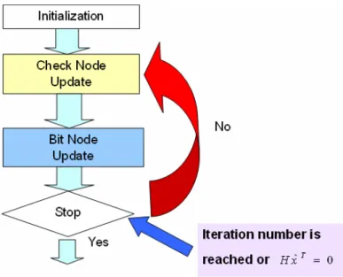
Otherwise, it goes to step1 until the parity-check equation is procured or the specific maximum iteration number is reached. The whole LDPC decoding procedure can be expressed in Figure 2.12.
Figure 2.12 The whole LDPC decoding procedure
Table 2.4 Summary of sum-product algorithm 1. Initialization:
2. Message passing:
Step1: Message passing from check nodes to variable nodes. For each ml, ,
compute 2 2 , 1 ( 0 ) 2
ln , w h ere is th e n o ise varian ce
( 1) , 1 l l l l l l m l m l l F o r l n P y x L y P y x F o r e v e r y l m s u c h th a t H q L σ σ → ≤ ≤ = = = = = = ' ' ( )\ ( ) l m m l l L m l r→