國 立 交 通 大 學
電信工程學系碩士班
碩 士 論 文
以外來資訊轉換圖設計調變器映射規則於
位元交錯調變碼之迭代解碼系統
EXIT-Chart Based Labeling Design for
Bit-interleaved Coded Modulation
with Iterative Decoding
指導教授:沈文和 博士
研 究 生:王楚硯
以外來資訊轉換圖設計調變器映射規則於
位元交錯調變碼之迭代解碼系統
EXIT-Chart Based Labeling Design for
Bit-interleaved Coded Modulation
with Iterative Decoding
研 究 生 : 王楚硯 Student : Chu-Yan Wang
指導教授 : 沈文和 博士 Advisor : Dr. Wern-Ho Sheen
國 立 交 通 大 學
電 信 工 程 學 系 碩 士 班
碩 士 論 文
A Thesis
Submitted to Department of Communication Engineering
College of Electrical and Computer Engineering
National Chiao Tung University
in Partial Fulfillment of the Requirements
for the Degree of
Master of Science
in Communication Engineering
July 2007
Hsinchu, Taiwan, Republic of China
中華民國九十六年七月
以外來資訊轉換圖設計調變器映射規則於
位元交錯調變碼之迭代解碼系統
研究生: 王楚硯 指導教授: 沈文和 博士
國立交通大學
電信工程學系碩士班
摘要
本論文利用外來資訊轉換圖 (Extrinsic Information Transfer Chart,EXIT- Chart) 聯合設計調變器映射規則 (Labeling) 與外部編碼器以增進位元交錯調變 碼之迭代解碼系統 (Bit-Interleaved Coded Modulation with Iterative Decoding, BICM-ID) 的性能。針對均勻的調變星座,我們提出一個有系統的調變星座映射 規則的設計方法以得到一組具有好的外來資訊轉換圖特性的映射規則;對每一種 外部編碼器皆可以從中選擇出一個最理想的映射規則,使解調器和解碼器的轉換 特性曲線能相交在外來資訊轉換圖上越遠的位置而且讓區線間的通道能夠打開 以達到理想的錯誤率。我們還擴展此映射規則設計方法到多維度的調變星座上, 多維度調變星座將一群位元映射到一組以一維度星座調變的符號使系統的設計 上具有更高的彈性與潛在性能的提升。經由模擬結果證實我們的設計比傳統的設
EXIT-Chart Based Labeling Design for Bit-interleaved
Coded Modulation
with Iterative Decoding
Student: Chu-Yan Wang
Advisor: Dr. Wern-Ho Sheen
Department of Communication Engineering
National Chiao Tung University
Abstract
In this thesis, constellation labeling is jointly designed with the outer code by using an EXIT-chart based analysis to improve the performance of bit-interleaved coded modulation with iterative decoding (BICM-ID). A systematic design method is proposed to obtain a set of labelings with good EXIT-chart characteristics for the regular one-dimensional (complex) modulation. Given an outer code, the best matched labeling can be employed to improve the BER performance. Furthermore, the method is extended to the multi-dimensional modulation case, where a group of bits are mapped to a vector of one-dimensional complex symbols. This general mapping strategy allows for more flexibility and potential performance improvements. Verified by the simulation results, our design provides a significant SNR gain over the conventional ones.
誌謝
首先要感謝我的指導教授 沈文和博士細心教導做研究的方法,不斷鼓勵學生 精益求精;老師嚴謹認真的求學態度一直是我們的最好的榜樣,讓我從研究過程 得到很多,對以後也有很大的幫助。感謝 王忠炫博士的教誨,老師不時的提醒 及激發學生的想法都讓學生受益匪淺。老師們每次 meeting 的建議都是學生研究 最大動力來源,使得這篇論文可以順利完成。 這篇論文主要是接著益彰學長的論文再加以改良,感謝學長之前辛苦的找出 這一個可以發揮的題目,讓我可以專心地想辦法解決問題;謝謝王老師、倉緯學 長幫忙寫 ISIT 的論文使能順利發表。也感謝這兩年來在實驗室所有的同學,正 欣學長、志成學長、宜康學長、香君學姊、鑫賢學長、順吉學長、東融學長、昱 帆學長、聖文學長、宸睿學長、相榮學長、文傑、友亮、小白、哲群、承瑋、政 揚、宜勳,感謝大家在各方面的幫助、照應,讓研究生活不單調。感謝在交大六 年來所有的師長、朋友,讓我增廣見聞。 最後要特別感謝我的爸媽的支持與照顧,爸媽辛苦的工作使我得以專心完成 學業,我一定會再更努力以報答我的家人。 民國九十六年七月Contents
摘要...i Abstract...ii 誌謝... iii Contents ...iv List of Tables...viList of Figures ...vii
Abbreviations...x
Chapter 1 Introduction ...1
1-1 Thesis Contributions...4
1-2 Thesis Organization ...5
Chapter 2 System Model...6
2-1 Transmitter...7
2-2 Channel model...8
2-3 Receiver ...9
2-3-1 Demapper ...9
2-3-2 Decoder ...11
Chapter 3 Exit-Chart Based Analysis ...12
3-1 Transfer Characteristics of Demapper ...12
3-2 Transfer Characteristics of Decoder ...16
3-3 Design Guideline Based on EXIT-chart ...17
Chapter 4 One-dimensional Labeling Design...21
4-1 Design criteria...21
4-1-1 Without A Priori Information ...22
4-1-2 Ideal A Priori Information ...24
4-1-2-1 AWGN Channels...24
4-1-2-2 Rayleigh Fading Channels ...26
4-2 Design Method ...28 4-3 Proposed Labelings...31 4-3-1 8-PSK ...31 4-3-2 16-QAM ...33 4-3-3 64-QAM ...35 4-4 Simulation Results...37
Chapter 5 Multi-dimensional Labeling Design...47
5-1-1 Multi-dimensional Mapping over Spatial Domain...48
5-1-1-1 Without A Priori Information ...48
5-1-1-2 Ideal A Priori Information...50
5-1-2 Multi-dimensional Mapping over Time Domain ...52
5-1-2-1 Without A Priori Information ...52
5-1-2-2 Ideal A Priori Information...52
5-2 Design Method ...56
5-3 Proposed Labelings...57
5-3-1 Multi-dimensional Mapping over Spatial Domain...57
5-3-1-1 N×BPSK...59
5-3-1-2 N×QPSK...62
5-3-1-3 N×8-PSK ...64
5-3-1-4 N×16-QAM ...65
5-3-2 Multi-dimensional Mapping over Time Domain ...66
5-3-2-1 N×BPSK...67
5-3-2-2 N×QPSK...72
5-3-2-3 N×8-PSK ...75
5-3-2-4 N×16-QAM ...77
5-4 Simulation Results...79
5-4-1 Multi-dimensional Mapping over Spatial Domain...79
5-4-2 Multi-dimensional Mapping over Time Domain ...87
Chapter 6 Conclusions ...96
List of Tables
Table 4-1 Candidate set for 8-PSK ...31
Table 4-2 Candidate set for 16-QAM ...33
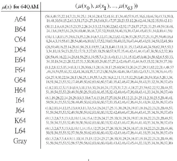
Table 4-3 Candidate set for 64-QAM ...35
Table 5-1 Summary of design criteria...56
Table 5-2 Candidate set for 2xBPSK ...59
Table 5-3 Candidate set for 3xBPSK ...60
Table 5-4 Candidate set for 4xBPSK ...61
Table 5-5 Candidate set for 2xQPSK...62
Table 5-6 Candidate set for 3xQPSK...63
Table 5-7 Candidate set for 2x8-PSK ...64
Table 5-8 Candidate set for 2x16-QAM ...65
Table 5-9 Candidate set for 2xBPSK ...67
Table 5-10 Candidate set for 3xBPSK ...69
Table 5-11 Candidate set for 4xBPSK ...70
Table 5-12 Candidate set for 2xQPSK...72
Table 5-13 Candidate set for 3xQPSK...73
Table 5-14 Candidate set for 2x8-PSK ...75
List of Figures
Fig. 1-1 Block diagram of BICM systems ...2
Fig. 1-2 Block diagram of BICM-ID systems ...2
Fig. 2-1 System model ...6
Fig. 3-1 Demapper transfer curve of Gray labeling for 16QAM in AWGN channel ..15
Fig. 3-2 Demapper transfer curve of Anti-Gray labeling for 16QAM in AWGN channel ...15
Fig. 3-3 Decoder transfer curves of turbo code and convolutional codes ...17
Fig. 3-4 An example of the EXIT-chart for BICM-ID at Eb /N0=4dB in AWGN channel ...18
Fig. 3-5 ObservationⅠfor labeling design. ...19
Fig. 3-6 Observation Ⅱ for labeling design ...20
Fig. 4-1 Two mappings of 8-PSK constellation: (a) Gray and (b) Set-partitioning...25
Fig. 4-2 Labelings for 8-PSK in Table 4-1 at (a) Eb /N0= 3dB in AWGN channel...32
Fig. 4-3 Labelings for 16-QAM in Table 4-2 at (a) Eb/N0= 3.5dB in AWGN channel ...34
Fig. 4-4 Labelings for 64-QAM in Table 4-3 at (a) at Eb/N0= 6dB in AWGN channel ...36
Fig. 4-5 (a) EXIT-chart at Eb/N0= 2.6dB and (b) performance plots of the BICM-ID system with 8-PSK and (5, 7) convolutional code in AWGN channel ...38
Fig. 4-6 (a) EXIT-chart at Eb/N0= 3dB and (b) performance plots of the BICM-ID system with 8-PSK and (133, 171) convolutional code in AWGN channel ...39
Fig. 4-7 (a) EXIT-chart at Eb/N0= 4.8dB and (b) performance plots of the BICM-ID system with 8-PSK and (133, 171) convolutional code in Rayleigh channel ...40
Fig. 4-8 (a) EXIT-chart at Eb/N0= 3.5dB and (b) performance plots of the BICM-ID system with 16-QAM and (5, 7) convolutional code in AWGN channel ...41
Fig. 4-9 (a) EXIT-chart at Eb/N0= 4dB and (b) performance plots of the BICM-ID system with 16-QAM and (133, 171) convolutional code in AWGN channel ...42
Fig. 4-10 (a) EXIT-chart at Eb/N0= 5.2dB and (b) performance plots of the BICM-ID system with 16-QAM and (133, 171) convolutional code in Rayleigh channel...43
Fig. 4-11 (a) EXIT-chart at Eb/N0= 6dB and (b) performance plots of the BICM-ID system with 64-QAM and (5, 7) convolutional code in AWGN channel ...44
system with 64-QAM and (133, 171) convolutional code in Rayleigh channel...46 Fig. 5-1 Equivalent and convenient model of the multi-dimensional mapper over spatial domain ...58 Fig. 5-2 Constituent two-dimensional mappers: (a) BPSK (b) QPSK (c) 8-PSK (d)
16-QAM and (e) 64-QAM...58 Fig. 5-3 Labelings for 2xBPSK in Table 5-2 at Eb /N0= 2dB in 2x2 fast Rayleigh fading channel...59 Fig. 5-4 Labelings for 3xBPSK in Table 5-3 at Eb /N0= 2dB in 3x3 fast Rayleigh fading channel...60 Fig. 5-5 Labelings for 4xBPSK in Table 5-4 at Eb /N0= 2dB in 4x4 fast Rayleigh fading channel...61 Fig. 5-6 Labelings for 2xQPSK in Table 5-5 at Eb/N0= 3dB in 2x2 fast Rayleigh fading channel...62 Fig. 5-7 Labelings for 3xQPSK in Table 5-6 at Eb/N0= 3dB in 3x3 fast Rayleigh fading channel...63 Fig. 5-8 Labelings for 2x8-PSK in Table 5-7 at Eb/N0= 5dB in 2x2 fast Rayleigh
fading channel...64 Fig. 5-9 Labelings for 2x16-QAM in Table 5-8 at Eb/N0= 6dB in 2x2 fast Rayleigh
fading channel...66 Fig. 5-10 Equivalent and convenient model of the multi-dimensional mapper over time domain ...67 Fig. 5-11 Labelings for 2xBPSK in Table 5-9 at (a) at Eb/N0= 1dB in AWGN channel and (b) Eb/N0= 3dB in block Rayleigh fading channel ...68 Fig. 5-12 Labelings for 3xBPSK in Table 5-10 at (a) at Eb/N0= 1dB in AWGN channel and (b) Eb/N0= 3dB in block Rayleigh fading channel ...70 Fig. 5-13 Labelings for 4xBPSK in Table 5-11 at (a) Eb/N0= 1dB in AWGN channel
and (b) Eb/N0= 3dB in block Rayleigh fading channel...71 Fig. 5-14 Labelings for 2xQPSK in Table 5-12 at (a) Eb /N0= 1dB in AWGN channel
and (b) Eb/N0= 3dB in block Rayleigh fading channel...73 Fig. 5-15 Labelings for 3xQPSK in Table 5-13 at (a) Eb /N0= 1dB in AWGN channel
and (b) Eb/N0= 3dB in block Rayleigh fading channel...74 Fig. 5-16 Labelings for 2x8-PSK in Table 5-14 at (a) Eb /N0= 3dB in AWGN channel
and (b) Eb/N0= 5dB in block Rayleigh fading channel...76 Fig. 5-17 Labelings for 2x8-PSK in Table 5-15 at (a) Eb/N0= 3.5dB in AWGN channel and (b) Eb/N0= 6dB in block Rayleigh fading channel...78 Fig. 5-18 (a) EXIT-chart at Eb/N0= 2dB and (b) performance plots of the BICM-ID
system with (5, 7) convolutional code in 2x2 fast Rayleigh fading channel...80 Fig. 5-19 (a) EXIT-chart at Eb/N0= 2dB and (b) performance plots of the BICM-ID
system with (5, 7) convolutional code in 3x3 fast Rayleigh fading channel...81 Fig. 5-20 (a) EXIT-chart at Eb/N0= 2dB and (b) performance plots of the BICM-ID
system with (5, 7) convolutional code in 4x4 fast Rayleigh fading channel...82 Fig. 5-21 (a) EXIT-chart at Eb/N0= 3dB and (b) performance plots of the BICM-ID
system with (5, 7) convolutional code in 2x2 fast Rayleigh fading channel...83 Fig. 5-22 (a) EXIT-chart at Eb/N0= 3dB and (b) performance plots of the BICM-ID
system with (5, 7) convolutional code in 3x3 fast Rayleigh fading channel...84 Fig. 5-23 (a) EXIT-chart at Eb/N0= 5dB and (b) performance plots of the BICM-ID
system with (5, 7) convolutional code in 2x2 fast Rayleigh fading channel...85 Fig. 5-24 (a) EXIT-chart at Eb/N0= 6dB and (b) performance plots of the BICM-ID
system with (5, 7) convolutional code in 2x2 fast Rayleigh fading channel...86 Fig. 5-25 (a) EXIT-chart at Eb/N0= 1dB and (b) performance plots of the BICM-ID
system with (5, 7) convolutional code in 1x1 AWGN channel ...88 Fig. 5-26 (a) EXIT-chart at Eb/N0= 3dB and (b) performance plots of the BICM-ID
system with (5, 7) convolutional code in 1x1 block Rayleigh fading channel...89 Fig. 5-27 (a) EXIT-chart at Eb/N0= 1dB and (b) performance plots of the BICM-ID
system with (5, 7) convolutional code in 1x1 AWGN channel ...90 Fig. 5-28 (a) EXIT-chart at Eb/N0= 3dB and (b) performance plots of the BICM-ID
system with (5, 7) convolutional code in 1x1 block Rayleigh fading channel...91 Fig. 5-29 (a) EXIT-chart at Eb/N0= 2.6dB and (b) performance plots of the BICM-ID
system with (5, 7) convolutional code in 1x1 AWGN channel ...92 Fig. 5-30 (a) EXIT-chart at Eb/N0= 5dB and (b) performance plots of the BICM-ID
system with ...93 Fig. 5-31 (a) EXIT-chart at Eb/N0= 3.5dB and (b) performance plots of the BICM-ID
system with (5, 7) convolutional code in 1x1 AWGN channel ...94 Fig. 5-32 (a) EXIT-chart at Eb/N0= 6dB and (b) performance plots of the BICM-ID
Abbreviations
APP A Posteriori Probability
AWGN Additive White Gaussian Noise BER Bit Error Rate
BICM Bit-Interleaved Coded Modulation
BICM-ID Bit-Interleaved Coded Modulation with Iterative Decoding
BI-STCM-ID Bit-Interleaved Space-Time Coded Modulation with Iterative Decoding BPSK Binary Phase Shift Keying
BSA Binary Switching Algorithm CSI Channel State Information
dB Decibel
EFF Error-free Feedback
FED Free Squared Euclidean Distance EXIT Extrinsic Information Transfer
LLR Log-Likelihood Ratio
MAP Maximum A Posteriori Probability MIMO Multi-Input Multi-Output
ML Maximum Likelihood
PEP Pairwise Error Probability PSK Phase-shift Keying
QAM Quadrature Amplitude Modulation QAP Quadratic Assignment Problem QPSK Quadrature Phase Shift Keying SISO Single-Input Single-Output SNR Signal-to-Noise Ratio TCM Trellis-Coded Modulation
Chapter 1
Introduction
Coded-modulation is a bandwidth-efficient scheme for data transmission on a bandwidth-limited channel. With joint design of coding and modulation, coded- modulation imposes no extra system bandwidth while achieves a coding gain comparable to the traditional coded system. Trellis-Coded Modulation (TCM) [1], proposed by Ungerboeck, is a form of coded modulation designed for additive white Gaussian (AWGN) channels, where the minimum free Euclidean distance (FED) of the coded symbol sequences determines the asymptotic BER performance. In [1], with a set-partitioning principle, TCM was designed with the largest FED by maximizing the intra-subset minimum Euclidean distance. Nevertheless, when transmitting over fading channels, the TCM performance will be degraded because in this case diversity order rather than the minimum FED becomes the primary factor that determines the BER performance [2].
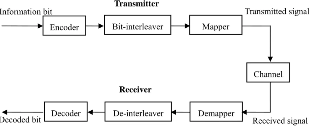
An approach to improve the performance coded-modulation systems in fading channels is to use bit-interleaved coded modulation (BICM) [3], [4]. BICM is a serial concatenation of a conventional channel code (called the outer code) and a mapper (called the inner code) with a bit-wise interleaver inserted between them, as shown in Fig. 1.1. The bit-wise interleaver can break the fading correlations and increase the diversity order to the minimum Hamming distance of the code at the expense of
decoding as two steps because joint demodulaton and decoding is too complicated to implement, and in [4], Caire laid a theoretic foundation on BICM, provided tools for evaluating its performance and gave design guidelines.
Fig. 1-1 Block diagram of BICM systems
Motivated by the serial concatenated structure of BICM, BICM with iterative decoding (BICM-ID) was proposed in [5], [6], [7] to improve the performance. The block diagram of a typical BICM-ID is shown in Fig. 1-2. Iterative decoding iteratively exchanges information between demapper and decoder. Through iterative decoding and with a proper labeling, the minimum inter-signal Euclidean distance of BICM is increased while the desired Hamming distance is preserved [6]. Therefore, BICM-ID can provide excellent performance in both AWGN and fading channels.
Fig. 1-2 Block diagram of BICM-ID systems
Encoder Bit-interleaver De-interleaver Decoder Demapper Mapper Received signal Channel Transmitted signal Information bit Transmitter
Receiver Decoded bit Encoder Bit-interleaver De-interleaver Decoder Bit-interleaver Demapper Mapper Channel Transmitted signal Information bits Transmitter
Receiver
It was shown in [4], [6], [7] that constellation labeling is crucial to the performance of BICM and BICM-ID systems. In [4], Gray labeling was proved to provide the best performance for BICM. In [6]-[7], different labelings were shown to have different influences on the bit error rate (BER) performance of BICM-ID. To find the optimal labeling for BICM-ID, the BER bounds of BICM [4] were extended in [6]-[7] with the assumption of error free feedback (EFF) to provide insight into the design of labeling. Their results suggest that the minimum Euclidean distance between any pairs of modulated symbols which have only one distinct bit on their labels should be maximized to minimize the BER upper bound at high signal-to-noise ratio (SNR). Beside, labeling design based on the extrinsic information transfer (EXIT) chart [8]-[10] indicates that under EFF assumption, the larger mutual information of demapper outputs is, the better asymptotic performance can be achieved.
Based on these criteria, many one-dimensional labelings for regular complex constellations (e.g., phase-shift keying (PSK) and quadrature amplitude modulation (QAM)) have been introduced. In [6]-[7], the authors use random computer search to choose a labeling that has reasonable first round performance and large iterative decoding gain to achieve low BER through several iterations. In [11], a general design algorithm based on binary switching algorithm (BSA) was proposed to find optimum labelings which can achieve the best asymptotic performance. The labeling optimization problem in [12] is solved by applying the generic solutions to the quadratic assignment problem (QAP) to achieve the largest asymptotic coding gain.
multi-dimensional modulation in single-input single-output (SISO) systems (i.e., the multi-dimensional signal is transmitted over consecutive time slots) and multi-input multi-output (MIMO) systems (i.e., the multi-dimensional signal is transmitted over distinct antennas), respectively. Labeling designs in [15]-[18] are based on the distance criteria deprived from the BER bounds to achieve best asymptotic performance. In [13]-[14], the authors use the EXIT-chart to design the labelings that are high at two end points of its demapper transfer curve to achieve good trade-off between the waterfall region and the BER floor.
1-1 Thesis Contributions
In terms of the EXIT-chart, given an outer code, a good labeling should be designed to form a tunnel between the transfer curve of demapper and decoder at SNR as low as possible to guarantee a low open tunnel threshold for BICM-ID. The demapper curve should also intersect the decoder curve at a point with mutual information as large as possible to avoid the undesired error floor at high SNR. However, labelings obtained in the previous works are designed separately from the outer code. The expected optimal performance hence can not always be achieved as different outer codes are employed. In most of the cases, those labelings perform well only at high SNR while unacceptable BER degradation is observed in the low SNR region. Given an outer code, we are to design the labeling to achieve the acceptable BER performance in the low SNR region.
In this thesis, therefore, constellation labeling is jointly designed with the outer code by an EXIT-chart based analysis. For an outer code, we observe that the demapper transfer curve of a good labeling should match to the decoder transfer curve and be high at its two end points to avoid early crossing with the decoder curve at low SNR and to achieve low BER after several iterations. In addition, we also observe that for different outer codes, the best labeling is different from code to code. Stimulated the above observations, a systematic methodology of labeling design is proposed for both one-dimensional and multi-dimensional modulation schemes which can easily obtain a set of labelings (called the candidate set) with good EXIT-chart characteristics. Given an outer code, we can then choose a labeling from the candidate set which is most matched to the outer code. Verified by the simulation results, our design can provide remarkable SNR gain over the conventional ones.
1-2 Thesis Organization
The rest of this thesis is organized as follows. In chapter 2, we describe the system model of BICM-ID. A brief review of the EXIT-chart based analysis as well as the basic guidelines of labeling design are given in chapter 3. A systematic design methodology for one-dimensional labeling is presented in chapter 4. The design methodology is extended in chapter 5 for multi-dimensional labeling. Simulation results are provided in chapter 4 and chapter 5 for one-dimensional and multi-dimensional designs, respectively, to verify the superiority of our design. Finally, a summary is drawn in chapter 6 to conclude this work.
Chapter 2
System Model
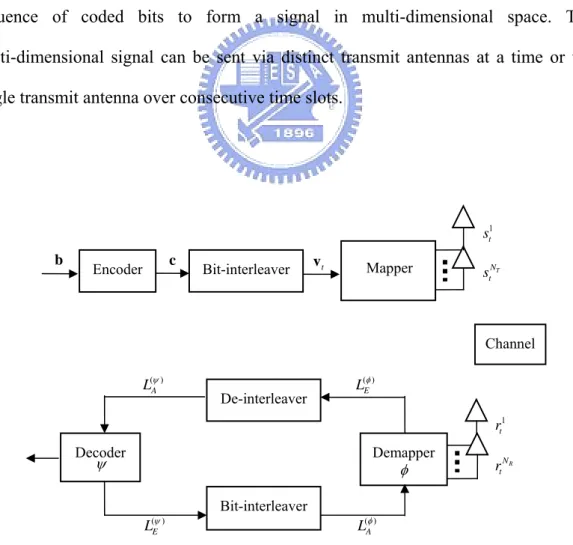
As mentioned in chapter 1, both one-dimensional and multi-dimensional constellations can be used in BICM-ID. This thesis is to provide a systematic labeling design for both one-dimensional and multi-dimensional complex constellations. The general system model with NT transmit antennas and NR receive antennas is shown in Fig. 2-1. When employing multi-dimensional constellation, the mapper maps a sequence of coded bits to form a signal in multi-dimensional space. The multi-dimensional signal can be sent via distinct transmit antennas at a time or via single transmit antenna over consecutive time slots.
Fig. 2-1 System model
Demapper Encoder Mapper Channel Bit-interleaver Bit-interleaver De-interleaver Decoder ( ) E Lφ ( ) A Lφ ( ) E Lψ ( ) A Lψ φ ψ t v 1 t s T N t s 1 t r R N t r b c
When employing one-dimensional constellation and reducing the number of transmit antenna and receive antenna to one, the model is reduced to a conventional BICM-ID system. The detailed system model is to be introduced in this chapter.
2-1 Transmitter
When a N-dimensional constellation is considered, a sequence of information bits b are encoded to c and then interleaved and grouped into to blocks
of mN coded bits; the t-th block is denoted vt =( [0],..., [vt v mNt ]). Then, vt is
mapped to a vector of symbols ( ,...,1 N)
t = st st
s , where each element of st is in a
one-dimensional complex constellation with =2m
M signal points. The signal st is in
a N-dimensional constellation χ which has M signal pointsN x ,0 x ,…,1 xMN−1and is equipped with a labeling μ which assigns xi a unique label ( )μ xi with
0 ( ) N
i M
μ
≤ x < . By setting N =NT , the -dimensionalN signal st is sent via NT transmit antennas at a time and received by NR antennas. If NT = 1 and 1NR = , the N-dimensional signal st is transmitted in a SISO channel over N consecutive time slots. Furthermore, when employing one-dimensional
constellation and setting NT = ,1 NR = , the model is reduced to a conventional 1 BICM-ID system and the transmitter parameters described above can also be applied in this case by setting N =1. Therefore, we will discuss the most general system
model employing multi-dimensional modulation with N transmit antennas and T N R receive antennas in the following.
2-2 Channel model
Assume the N-dimensional signal st is transmitted via NT antennas over a flat fading channel H , where N =NT . Each element of the NR×NT matrix H is assumed to be zero-mean i.i.d. complex Gaussian distributed with variance 1/2 per dimension. Let =( ,...,1 )
r NR
t rt rt represent the received signal corresponding to st and rt is given by
= +
rt Hst nt (2-1)
where nt is a vector of noise with zero mean and variance N0/ 2 per dimension. On the other hand, if st is transmitted via single antenna over N consecutive time slots
over a flat fading channel and received by single antenna, the received signal corresponding to st is denoted rt =( ,...,rt1 rtN) and rtp is given by
α = + p p p p t t t t r s n (2-2) where αp
t denotes the channel gain, p t
n stands for the noise with zero mean and variance / 2 N0 per dimension and 1≤ ≤p N . If setting fading coefficients equal to 1, it becomes an AWGN channel. Moreover, when employing one-dimensional constellation and setting NT = ,1 NR = , the model is reduced to a conventional 1 BICM-ID system. The system model is given by
α
= +
t t t t
r s n (2-3)
2-3 Receiver
The demapper φ takes rt’s and the a priori input ( )φ ( [ ])
A t
L v i ’s (i.e., the log- likelihood ratio (LLR) of [ ]v i ’s fed back from the decodert ψ ) and then compute the extrinsic output by [12] ( )( [ ]) ln Pr( [ ] 1| ) ( )( [ ]) Pr( [ ] 0 | ) φ = = − φ = r r t t E t A t t t v i L v i L v i v i
(
)
(
)
1 0 2 ( ) 0 2 ( ) t 0 exp [ ] [ ] ln exp [ ] [ ] i t i t t t t A t j i t t A t j i v j L v j N v j L v j N φ χ φ χ ≠ ∈ ≠ ∈ ⎧ − ⎫ ⎪− + ⎪ ⎨ ⎬ ⎪ ⎪ ⎩ ⎭ = ⎧ − ⎫ ⎪− + ⎪ ⎨ ⎬ ⎪ ⎪ ⎩ ⎭∑
∑
∑
∑
s s r Hs r Hs (2-4) where i bχ is the subset of χ comprising all the multi-dimensional signal points for those the i-th bit of the binary representation of their labels is of value b. Note that
( )φ ( [ ])
E t
L v i ’s also depend on the choices of χ and μ . The output LLRs of the demapper are then de-interleavedand serve as the a priori inputs ( )ψ ( [ ])
A t
L v i 's of the
decoder. Finally, the extrinsic outputs ( )ψ ( [ ])
E t
L v i 's of the decoder generated by an appropriate soft-input soft-output decoding algorithm, e.g. BCJR algorithm [19], are fed to the demapper for next iteration of processing. The derivations of extrinsic information at demapper output and decoder output will be introduced in the next two subsections, respectively.
2-3-1 Demapper
Pr( [ ] 1| ) ln Pr( [ ] 0 | ) = = r r t t t t v i v i Pr( [ ] 1) Pr( | [ ] 1) ln ln Pr( [ ] 0) Pr( | [ ] 0) = = = + = = r r t t t t t t v i v i v i v i Pr( [ ] 1) Pr( ; [ ] 1) / Pr( [ ] 1) ln ln Pr( [ ] 0) Pr( ; [ ] 0) / Pr( [ ] 0) = = = = + = = = r r t t t t t t t t v i v i v i v i v i v i 1 0 Pr( ; ) / Pr( [ ] 1) Pr( [ ] 1) ln ln Pr( [ ] 0) Pr( ; ) / Pr( [ ] 0) χ χ ∈ ∈ = = = + = =
∑
∑
s s r s r s i t i t t t t t t t t t v i v i v i v i 1 0 Pr( | ) Pr( ) / Pr( [ ] 1) Pr( [ ] 1) ln ln Pr( [ ] 0) Pr( | ) Pr( ) / Pr( [ ] 0) χ χ ∈ ∈ ⎡ ⎤ ⋅ = ⎢ ⎥ = ⎢⎣ ⎥⎦ = + = ⎡ ⎤ ⋅ = ⎢ ⎥ ⎢ ⎥ ⎣ ⎦∑
∑
s s r s s r s s i t i t t t t t t t t t t t v i v i v i v i 1 0 1 0 1 0 Pr( | ) Pr( [ ]) / Pr( [ ] 1) Pr( [ ] 1) ln ln Pr( [ ] 0) Pr( | ) Pr( [ ]) / Pr( [ ] 0) χ χ − = ∈ − = ∈ ⎡ ⎤ ⋅ = ⎢ ⎥ = ⎢⎣ ⎥⎦ = + = ⎡ ⎤ ⋅ = ⎢ ⎥ ⎢ ⎥ ⎣ ⎦∑
∏
∑
∏
s s r s r s t i t t i t mN t t t t j t mN t t t t t j v j v i v i v i v j v i 1 0 1 0, 1 0, Pr( | ) Pr( [ ]) Pr( [ ] 1) ln ln Pr( [ ] 0) Pr( | ) Pr( [ ]) χ χ − = ≠ ∈ − = ≠ ∈ ⎡ ⎤ ⋅ ⎢ ⎥ = ⎢⎣ ⎥⎦ = + = ⎡ ⎤ ⋅ ⎢ ⎥ ⎢ ⎥ ⎣ ⎦∑
∏
∑
∏
s s r s r s t i t t i t mN t t t j j i t mN t t t t j j i v j v i v i v j 1 0 2 ( ) 0 ( ) 2 ( ) 0 exp{ [ ] ( [ ])} ( [ ]) ln exp{ [ ] ( [ ])} φ χ φ φ χ ≠ ∈ ≠ ∈ − − + = + − − +∑
∑
∑
∑
t s t s r Hs r Hs i t i t t t A t j i A t t t A t j i v j L v j N L v i v j L v j N (2-5)where in the last equation
( )( [ ]) ln Pr( [ ] 1) Pr( [ ] 0) φ = = = t A t t v i L v i v i (2-6)
and form equation (2-1) the likelihood function is given by
2 0 0 1 exp Pr( | ) (π ) ⎡ ⎤ − ⋅ − ⎢ ⎥ ⎣ ⎦ = t t t t r Hs r s R N N N . (2-7)
For the first round iteration, no a prior LLR is available and hence ( )φ ( [ ]) 0, = ∀
A t
L v i i .
The demapper outputs the extrinsic a posteriori LLR ( )φ ( [ ])
E t L v i ’s, where ( )( [ ]) lnPr( [ ] 1| ) ( )( [ ]) Pr( [ ] 0 | ) φ = − φ = r r t t E t A t t t v i L v i L v i v i 1 0 2 ( ) 0 2 ( ) 0 exp{ [ ] ( [ ])} ln exp{ [ ] ( [ ])} φ χ φ χ ≠ ∈ ≠ ∈ − − + = − − +
∑
∑
∑
∑
t s t s r Hs r Hs i t i t t t A t j i t t A t j i v j L v j N v j L v j N , (2-8)and then the soft-output ( [ ])( )φ
E t
L v i ’s are de-interleaved and serve as the a priori inputs ( [ ])( )ψ
A
L c i 's of the decoder.
2-3-2 Decoder
The decoder takes ( [ ])( )ψ A
L c i ’s and computes the a posteriori LLR of coded bits
( ) ( ) Pr( [ ] 1| ) ln Pr( [ ] 0 | ) ψ ψ = = A A c i L c i L (2-9)
and the a posteriori LLR of information bits
( ) ( ) Pr( [ ] 1| ) ln Pr( [ ] 0 | ) ψ ψ = = A A b i L b i L (2-10)
by an appropriate soft-input soft-output decoding algorithm, e.g. BCJR algorithm. The decoder produces the extrinsic a posteriori LLR ( )ψ ( [ ])
E L c i ’s, where ( ) ( ) ( ) ( ) Pr( [ ] 1| ) ( [ ]) ln ( [ ]) Pr( [ ] 0 | ) ψ ψ ψ ψ = = − = A E A A c i L L c i L c i c i L , (2-11) and ( [ ])( )ψ E
L c i ’s are interleaved and serve as the a priori inputs L( )Aφ ( [ ])v i 's of the t demapper.
Chapter 3
Exit-Chart Based Analysis
The EXIT chart is a powerful tool for analyzing the convergence behavior of iterative decoding schemes [8], [9], [20], which consists of two parallel or serial concatenated soft-input soft-output decoders. We use the EXIT chart for performance analysis to trace the effect of μ on BICM-ID, where two transfer characteristics for decoder and demapper are plotted in the same diagram. Each curve describes how the mutual information between input LLRs and transmitted bits transfers to that between output LLRs and transmitted bits. The transfer characteristics of demapper and decoder as well as the labeling design guideline based on EXIT-chart will be discussed in the following sections.
3-1 Transfer Characteristics of Demapper
The demapper φ takes channel observations rt’s and a priori input
( )φ A
L ’s from
the decoder and calculates the extrinsic a posteriori ( )φ E
L ’s by equation (2-4). The information transfer can be controlled by the robustness of the a priori information. Several observations are obtained from [20]. 1) For large interleavers the a priori information ( )φ
A
L ’s remain fairly uncorrelated from the respective channel observations
t
r ’s over many iterations. 2) The probability density function of the a priori
information approach Gaussian-like distribution with increasing number of iterations. Therefore, it is appropriate to model the a priori input ( )φ
A
known transmitted upmapped bitv∈ ± as { 1}
( )
A A A
Lφ =μ ⋅ + , v n (3-1)
where nA is an independent Gaussian random variable with zero mean and variance
2 σA and according to [20] 2 2 σ μ = A A . (3-2)
The conditional probability density function of ( )φ A L is 2 2 2 ( ) (( ( 2) ) / 2 ) ( | ) 2 A A A v L A e p φ V v ξ σ σ ξ πσ − − ⋅ = = . (3-3)
To measure the information contents of the a priori information, the mutual information ( ;( ) ( ))
A A
I φ =I V Lφ between the transmitted bits V and the L-values L ’s is ( )Aφ used. ( ) ( ; ( )) A A I φ =I V Lφ ( ) ( ) ( ) ( ) 2 1,1 2 ( | ) 1 ( | ) log ( ) 2 ( | 1) ( | 1) A A A A L L v L L p V v p V v d p V p V φ φ φ φ ξ ξ ξ ξ ξ +∞ =− −∞ ⋅ = = = ⋅ = + = −
∑ ∫
(3-4) ( ) 0≤IAφ ≤1. (3-5)With equation (3-2) and (3-3), equation (3-4) becomes
2 2 2 (( ( 2) ) / 2 ) ( ) 2 ( ) 1 log (1 ) . 2 A v A A A A e I e d ξ σ σ φ σ ξ ξ πσ +∞ − − ⋅ − −∞ = −
∫
⋅ + (3-6)For abbreviation define
( )
( )σ = Aφ (σA =σ)
J I (3-7)
with
Thus, given an ( )φ A
I and a sequence of transmitted bits for a particular value of Eb/N , 0 we can use σA to generate the independent Gaussian random variables ( )φ
A
L ’s. At the demapper output, the mutual information ( ) ( ; ( ))
E E
I φ =I V Lφ between the transmitted bits V and the L-values ( )φ
E L ’s is calculated. ( ) ( ; ( )) E E I φ =I V Lφ ( ) ( ) ( ) ( ) 2 1,1 2 ( | ) 1 ( | ) log ( ) , 2 ( | 1) ( | 1) E E E E L L v L L p V v p V v d p V p V φ φ φ φ ξ ξ ξ ξ ξ +∞ =− −∞ ⋅ = = = ⋅ = + = −
∑ ∫
(3-10) ( ) 0≤IEφ ≤1. (3-11)Note that the required pdf ( |( ) )
E L
p φ ξ V = can be estimated by generating the histogram v of ( )φ
E
L and no Gaussian assumption is imposed on this term. Therefore, given an ( )φ
A
I and a Eb/N , the extrinsic information transfer characteristics can be 0 computed.
For example, Fig. 3-1 and Fig. 3-2 show the deampper transfer curves of Gray and Anti-Gray [21] labeling for 16QAM in AWGN channel respectively. It can be seen from these figures that the demapper curve is enhanced at all range of ( )φ
A
I but not equally at higher Eb/N . For Gray labeling, the transfer curve remains almost 0 constant with the increasing of ( )φ
A
I , whereas the transfer curve of Anti-Gray labeling is very steep revealing the potential performance improvement over iterations.
Fig. 3-1 Demapper transfer curve of Gray labeling for 16QAM in AWGN channel
3-2 Transfer Characteristics of Decoder
The decoder ψ takes the a priori input ( )ψ A
L ’s from the demapper and calculates the extrinsic a posteriori ( )ψ
E
L ’s by equation (2-10). Because there is no channel observations in the decoder input, its transfer characteristics do not depend on Eb/N . 0
Define the mutual information between the coded bits and the decoder input and between the coded bits and the decoder output as ( )ψ
A
I and IE( )ψ , respectively. Assume ( )ψ
A
L ’s are independent Gaussian distributed, the extrinsic information transfer characteristics of the decoder can be computed by the same way as presented in the previous section.
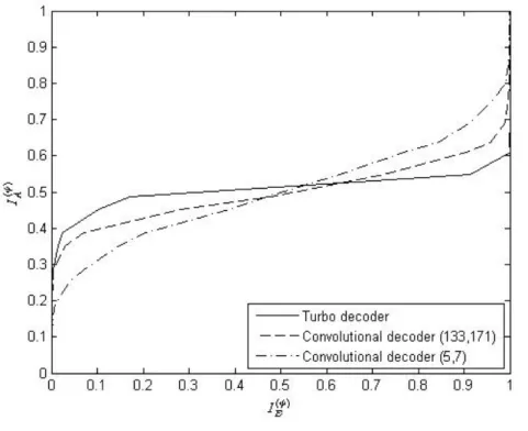
Fig. 3-3 shows an example of the decoder transfer curves of a rate-1/2 turbo code
[22], [23] with constituent code
2 3 3 1 1, 1 D D D D ⎛ + + ⎞ ⎜ + + ⎟
⎝ ⎠ and with 5 inner iterations as well
as two convolutional codes with generator matrix 2 2
(1+D ,1+ +D D ) and
2 3 5 6 2 3 6
(1+D +D +D +D ,1+ +D D +D +D ). Note that the axes are swapped: the input is in the ordinate and the output is in the abscissa. It can be seen from the figure that the larger the code memory is, the flatter the decoder curve will be and the farther the curve may intersect with the demapper curve. Then, the resulting BER
Fig. 3-3 Decoder transfer curves of turbo code and convolutional codes
3-3 Design Guideline Based on EXIT-chart
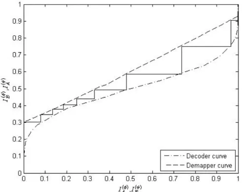
The transfer characteristics of the demapper and the decoder can be plotted in the same diagram with the axis of the decoder swapped. The exchange of extrinsic information between the demapper and the decoder can be visualized as the decoding trajectory in the EXIT-chart. Consider an example with the trajectory shown in Fig. 3-4, where ( ( ), ( ))
A E
I φ I φ and (IA( )ψ ,IE( )ψ ) denote the mutual information of input and output LLRs of the demapper and decoder, respectively. The trajectory shows how the mutual information actually transfers between the decoder and the demapper. The farthest point that the trajectory can reach is the first intersection of the decoder transfer curve and the demapper transfer curve and it determines the performance limit of BICM-ID system.
Fig. 3-4 An example of the EXIT-chart for BICM-ID at Eb/N0=4dB in AWGN channel
Given an outer code, a good labeling should be designed such that the demapper transfer curve and the decoder transfer curve can form a tunnel at SNR as low as possible to guarantee a low threshold for BICM-ID and have the first intersection at the farthest point to lower the undesired BER floor. Consider an example in Fig. 3-5, where two channel codes: a convolutional code with generator matrix
2 2
(1+D ,1+ +D D ) and a rate-1/2 turbo code with constituent code
2 3 3 1 (1, ) 1 + + + + D D
D D are investigated with two kinds of labelings: Gray and Anti-Gray [21] at Eb/N =4dB in AWGN channel. It can be observed from the figure that Gray is 0
preferable to the turbo code while Anti-Gray is favorite to the convolutional code. This example suggests that the best labeling is different form code to code and therefore the labeling should be designed jointly with the outer code. Consider another example in Fig. 3-6, where a convolutional code with generator matrix
2 3 5 6 2 3 6
labelings: MSEW [24] and M16a [11] at Eb/N =4.5dB in AWGN channel. The 0
MSEW is more preferred because the left-end point of its demapper curve is higher than that of M16a such that the tunnel can be opened at lower threshold and the right-end point is almost the same such that similar BER floor can be expected. This example advises that the transfer curve of the good labeling should be high at its two end points for an given outer code. Therefore, the design guideline can be summarized as: the best labeling should be designed such that its corresponding transfer curve not only matches a given outer code but is high at its two end points.
Fig. 3-6 Observation Ⅱ for labeling design
For a one-dimensional mapper with M signal points, an intuitive way to find the optimal labeling with respect to some outer codes is to plot the demapper curve of all possible !M labelings and then choose the one most matched to the outer code.
However, for a large M , the high complexity required for exhaustive search is usually far beyond what a practical system can afford. To provide a practical search scheme for the optimal labeling, a systematic design methodology is proposed in next chapter.
Chapter 4
One-dimensional Labeling Design
The design guideline based on the EXIT-chart in chapter 3 pointed out that the best labeling should be designed such that its corresponding transfer curve not only matches a particular outer code but is high at its two end points. In this chapter, labeling design for regular one-dimensional constellation is concerned and the system model is reduced from the general system model Fig. 2-1 by employing a 1-D mapper as well as setting NT = and 11 NR = . Several criteria regarding the highness of two end points of demapper transfer curve will be presented first and then a systematic design method based on these criteria is proposed to design a set of lablings with good EXIT-chart characteristics. In this chapter, a one-dimensional M-ary complex constellation with m=log2M is assumed.
4-1 Design criteria
The mutual information between the demapper output and the coded bits when no a priori information is available (denoted as IE( )φ
(
I( )Aφ =0)
) and when a priori information is ideally fed back (denoted as ( )(
( ) 1)
E A
I φ I φ = ) corresponds to the left-end and the right-end point of the demapper transfer curve, respectively. Several criteria deprived in previous works governing ( )
(
( ) 0)
E A
4-1-1 Without A Priori Information
When a priori information from the decoder is not available (i.e., IA( )φ =0), it corresponds to the first iteration when the demapper takes only the channel observations r ’s and computes the extrinsic a posteriori information ( )φ
E
L ’s by assuming the probability of occurrence of bit 1 and bit 0 are equal likely. Higher ( )φ
E
I corresponds with a lower BER Pb0 of the hard-decisioned bits at the demapper output. The derivation of 0
b
P is as follows. By the union bound approximation, the pairwise symbol error probability (p xl →xk) when xl is transmitted and erroneously decided as x can be written as k
1 0, ( ) − ( ) = ≠ → ≤
∑
M → l k l k k k l p x x p x x . (4-1)Then the averaged symbol error rate p can be written as e
1 1 0 0, ( ) ( ) − − = = ≠ =
∑ ∑
M M → ⋅ e l k l l k k l p p x x p x . (4-2)The relationship between the symbol error probability p and the bit error probability e eb
p of a MPSK or MQAM signal is as follows (assume the bit error probability in each bit position is equal likely)
1 = − e c p p 1 ( )m cb p = − 1 (1 ) = − − m eb p ( By Taylor's expansion) ≈ ⋅m peb (4-3)
By equation (4-2) and (4-3), 0 b P can be written as [14], [25]
0 1 1 0 0 ( ( ), ( )) Pr( ) Pr( ) μ μ − − = = ≠ =M
∑ ∑
M Ham l k → ⋅ b l k l l k k l d x x P x x x m(4-4)
where (.,.)dHam denotes the Hamming distance of two bit vectors and Pr( ) 1xl = M owing to the lack of a priori information.
At a Eb/N , the pairwise symbol error probability0 p x( l →xk)depends on the Euclidean distance between x andl x : as the distance becomes smaller, the pairwise k symbol error probability is larger. The nearest constellation points therefore contribute more in the symbol error probability and thus the BER 0
b
P . The average number of bits that differ between two closest constellation points is then the most important parameter that determines 0
b P , which is denoted as [14]
( ) ( )
(
)
1 0 1 1 , ( ) k l av Ham l k l x N d x x N l χ χ μ μ χ − = ∈ ⎡ ⎤ = ⎢ ⎥ ⎣ ⎦∑
∑
, (4-5)where χl contains the nearest neighbors of x andl χl =N l( ). Hence, Nav can be used to determine ( )
(
( ) 0)
E A
I φ I φ = . Note that Nav depends on μ and not on Eb/N0 and channel.
4-1-2 Ideal A Priori Information
When ideal a priori information from the decoder is available (i.e.,IA( )φ =1), the demapper computes the extrinsic a posteriori information ( )φ
E
L ’s based on the channel observations r ’s and the a priori information ( )φ
A
L ’s. Higher IE( )φ corresponds with a lower BER 1
b
P . The BER upper bounds deprived in [4], [6], [7] for AWGN channels and Rayleigh fading channels will be presented in this sections.
4-1-2-1 AWGN Channels
The union bound of probability of bit error for convolutional codes of rate /kc n c is given by [4] 1 1 ( ) ( , , ) , f b I d d c P W d f d k μ χ ∞ = ≤
∑
(4-6)where ( ) W dI is the total information weight of error events at Hamming distance d, df is the minimum Hamming distance of the code and ( , , ) f d μ χ is the average pairwise error probability (PEP) depending on Hamming distance d , a labeling μ and a signal constellation χ.
In AWGN channels, f d( , , ) μ χ is deprived as [4] [11]
2 1 1 0 0 1 ( , , ) exp 2 k k 4 b b d m m k b x z x z f d m χ χ N μ χ = = ∈ ∈ ⎡ ⎛ ⎞⎤ ⎢ ⎜ −⎜ ⎟⎟⎥ ⋅ ⎢ ⎝ ⎠⎥ ⎣
∑∑ ∑ ∑
⎦ -∼ , (4-7)where z is the only element in χk
b under the EFF assumption (i.e., other bits forming a channel symbol are known). For example, Fig. 4-1 shows the Gray labeling and the Set-partitioning labeling for 8-PSK; when a priori information is ideally fed back, the 8-PSK constellations can be partitioned into sets of BPSK constellations having larger
intersignal Euclidean distance. Therefore, equation (4-7) can be rewritten as 2 1 1 0 0 1 ( , , ) exp 2 k 4 b d m m k b x x z f d m χ N μ χ = = ∈ ⎡ ⎛ ⎞⎤ ⎢ ⎜ −⎜ ⎟⎟⎥ ⋅ ⎢ ⎝ ⎠⎥ ⎣
∑∑ ∑
⎦ -∼ . (4-8)It can be seen form equation (4-8) that ( , , ) f d μ χ is dominated by the terms with the smallest square Euclidean distance, which is denoted as
2 min , , min . k b x k b d x z χ ∈ ∀ = - (4-9)
The number of terms in equation (4-8) corresponding to dmincan be equivalently expressed, up to a scaling factor, as the average number of nearest neighbors [15]
2 1
min min min 0 1 ( , ) 2 m i m i N N x d − = =
∑
(4-10)where ( ,Nmin x di min) is the number of nearest neighbors of x . Note that bothi dminand
min
N depend on the mapping and constellation. If a labeling has larger dminand smaller Nmin, this labeling can achieve lower BER 1
b
P and higher IE( )φ
(
IA( )φ = in 1)
AWGN channel.4-1-2-2 Rayleigh Fading Channels
In [6] [7], the asymptotic performance of BICM-ID over Rayleigh fading channels can be approximated at high SNR by
(
)
1 2 10 0 log [ ] const 10 f b b dB dB d E P R N ⎛ ⎞ − Ω +⎜ ⎟ + ⎝ ⎠ (4-11)where df is the free Hamming distance of the code, R is the information rate (bits/dim)and Ω is the harmonic mean of the squared Euclidean distances, defined 2
as
(
)
1 1 2 1 2 m k=1 0 1 2 k b m b x x z m χ − − = ∈ ⎡ ⎤ Ω =⎢ − ⎥ ⎢ ⎥ ⎣∑∑ ∑
⎦ (4-12) where k bz∈χ and logm= 2M . Note that under EFF assumption z is the only element in χk
b . The performance bound over Rayleigh fading channels primary depends on df and Ω and is not dominated by the minimum intersignal Euclidean 2 distance as in AWGN channels. It can be seen form equation (4-11) that df controls the slope of the probability of bit error curve while Ω provides the horizontal offset. 2
Moreover, since df is a parameter of the channel code and Ω is a function of the 2 labeling μ and the signal set χ, the effect of the channel code and the labeling on BER 1
b
P can be separately optimized. If the minimum squared Euclidean distance between any pairs of modulated symbols which have only one distinct bit on their labels is increased, Ω is increased and the resulting BER2 1
b
P is lower. Then, IE( )φ is higher at the right-end point of the demapper transfer curve.
Hence we will investigate more on Ω in the following. For each signal point 2 i x , define
(
)
1 1 2 2 k=1 1 m i xi z m ω − − ⎛ − ⎞ ⎜ ⎟ ⎝∑
⎠ (4-13) where , k k i b bx ∈χ z∈χ . Each ωi2 is the harmonic mean of the squared Euclidean distances between x and otheri m constellation points whose labels differ in only
one bit-position with x . With this definition, we can rewritei Ω as the harmonic 2 mean of ω2 i ’s
( )
1 2 1 1 2 2 i=0 1 2 m i m ω − − − ⎡ ⎤ Ω = ⎢ ⎥ ⎣∑
⎦ . (4-14)If taking partial derivative of Ω with respect to2 2
i ω , the result is
( )
2 1 2 2 2 1 0, 2 1 1 2 2 2 0, 0 1 2 M j M j j i m j M M j j i i j k j k j ω ω ω ω ω − − = ≠ − − = ≠ = = + ⎛ ⎞ ⎜ ⎟ ⎛ ⎞ ∂Ω = ⋅⎜ ⎟ ∝ ⎜ ⎟ ⎜ ⎟ ∂ ⎝ ⎠ ⎜ ⎟ ⎝ ⎠∏
∏
∑ ∑
. (4-15) If ω2 i is the minimum in 2 ωi ’s, then ∂Ω ∂2 (ω2)i is maximized. Therefore, we learn that the increment of the smallest term of ω2
i ’s maximizes the increase of
2
Ω . The large increment of Ω lowers BER2 1
b
4-2 Design Method
Based on these design criteria regarding the highness of the two end points of the demapper transfer curve discussed in last section, we are ready to design a set of labelings (called the candidate set Γ ) with desired good EXIT-chart characteristics (i.e., the demapper transfer curve matches the decoder transfer curve and is as high as possible at its two end points). Conventional Gray labeling, whose transfer curve is almost flat since the minimum intersignal Euclidean distance can not be increased through iterative decoding, is first chosen as the initial labeling. It can be observed that the demapper curve will be steeper if swapping any two labels of the Gray labeling. To design labelings with good EXIT-chart characteristics, the two labels to be swapped should be selected such that ( )
(
( ) 1)
E A
I φ I φ = can be enhanced significantly and ( )
(
( ) 0)
E A
I φ I φ = can be pulled down least. Through consecutive label swappings, we can get a set of labelings with good EXIT-chart characteristics.
More specifically, to make ( )
(
( ) 1)
E A
I φ I φ = be enhanced significantly after swapping two labels in both AWGN and Rayleigh fading channels, the criteria presented in section 4-1-2 are used. In AWGN channels, larger dminand smaller Nmincan result in lower BER 1
b
P and higherIE( )φ . Each swapping must ensure that Nmincan be reduced and dmincan be gradually enlarged through consecutive swappings. Therefore, we require the signal point x to be swapped with anther one should satisfy i
2
min
min{ xi−xj :∀ ≠j i d, Ham( ( ), ( )) 1}μ xi μ xj = =d . (4-16) In Rayleigh fading channels, larger Ω can result in lower BER2 1
b
P and higher IE( )φ and the increasing of the smallest term of ω2
i ’s maximizes the increasing of
2
Because many small terms in ω2
i ’s are usually about the same value, each swapping must guarantee that one of them can be enlarged such that Ω can be increased 2
significantly. Therefore, the signal point x to be swapped with another one is also i required to satisfy
2 2
ωi ≤ Ω . (4-17)
On the other hand, to make ( )
(
( ) 0)
E A
I φ I φ = be pulled down least, the criterion presented in section 4-1-1 suggests that N should be kept small after each swapping. Based on av the above design principles, a systematic procedure is proposed as follows.
Procedure for searching Γ :
Step 1: Choose Gray mapping as the initial labeling. Step 2: Calculate ω2
i of each constellation point x andi
2
Ω .
Step 3: Generate a set of constellation points. Each one, say x , must satisfy equation i (4-16) and the corresponding ω2
i must satisfy equation (4-17).
Step 4: Try to switch the label of each signal point in the set with the label of another signal point in the constellation and then calculate the resulting '
av
N and Ω . '2 Step 5: Select a pair of signal points for label swapping and then store the resulting
labeling in Γ . The selection rule is as follows:
1. Over the pairs satisfying Ω > Ω , select the pair with minimum'2 2 '
av N . 2. If there are more than one pairs with the same minimum '
av
N , select the pair with maximum Ω . '2
3. If there are still more than one pairs with the same maximum Ω , pick any '2
one of them and store other pairs’ resulting labelings after swapping in a temporary stack.
Step 6: If the swapping pair can be found in Step5, go back to Step 2 and continue the search procedure. If not (i.e., all the swapping pairs’ corresponding Ω ≤ Ω ), '2 2
go to Step 7.
Step 7: Replace the initial labeling with one labeling stored in the temporary stack. Remove this one from the temporary stack. Then, restart the search procedure. Stop until the temporary stack is empty.
Remarks:
When the search procedure is finished, we can get many labelings in Γ . There are two points to be noted:
1. If there are more than one lableings in Γ with the same value of Ω and 2
av N , pick any one of them and discard others. These labelings may result in the same EXIT-chart characteristics and BER performance.
2. For those demapper transfer curves corresponding to the labelings in Γ , uniformly quantize ( )
(
( ) 0)
E A
I φ Iφ = . With each discrete value at the left end, choose the labeling with the largest ( )
(
( ) 1)
E A
4-3 Proposed Labelings
The searched Γ ’s for 8-PSK, 16-QAM and 64-QAM are presented in Table 4-1, 4-2, 4-3, respectively, where the labelings are listed in a decreasing order in terms of
(
)
( ) ( ) 1
E A
I φ I φ = . From Fig.4-2, Fig. 4-3 and Fig 4-4, the labeling are observed to generate the curves which are uniformly distributed in the left end and are high in the right end in both AWGN and Rayleigh fading channel. In addition, all the demapper curves can still keep the same order at various SNR and channel. Therefore, given an outer code, we can then choose a labeling form Γ which most matches the outer code to make tunnel open at low threshold and achieve acceptable BER at high SNR.
4-3-1 8-PSK
(a)
(b)
Fig. 4-2 Labelings for 8-PSK in Table 4-1 at (a) Eb/N0= 3dB in AWGN channel and (b) Eb /N0= 5dB in Rayleigh fading channel
4-3-2 16-QAM
(a)
(b)
Fig. 4-3 Labelings for 16-QAM in Table 4-2 at (a) Eb/N0= 3.5dB in AWGN channel and (b) Eb /N0= 6dB in Rayleigh fading channel
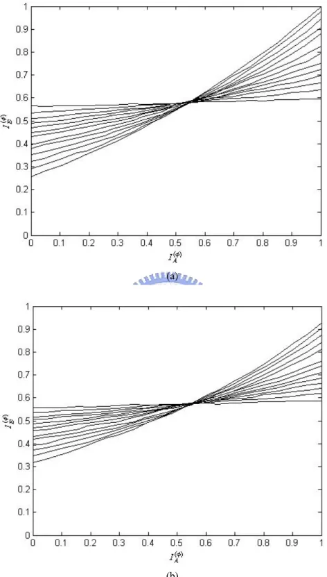
4-3-3 64-QAM
(a)
(b)
Fig. 4-4 Labelings for 64-QAM in Table 4-3 at (a) at Eb/N0= 6dB in AWGN channel and (b) Eb /N0= 8dB in Rayleigh fading channel
4-4 Simulation Results
To verify the superiority of our design over the conventional labelings, the BICM-ID system consisting of two kinds of rate-1/2 convolutional codes with generator matrix(1+ 2,1+ + 2)
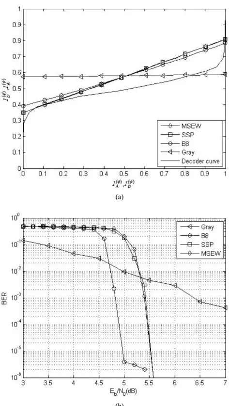
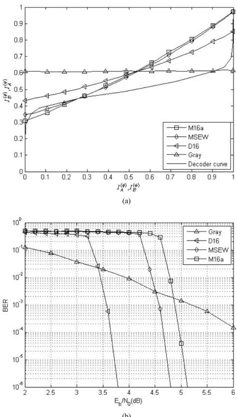
D D D and(1+D2+D3+D5+D6,1+ +D D2+D3+D6), a bit-interleaver of block length 24000 bits, and 8-PSK/16-QAM/64-QAM modulation is simulated for transmission over AWGN and Rayleigh channels. The demapper in (2-4) and BCJR decoder of the outer code are employed for iterative decoding with 40 iterations. For 8-PSK modulation, conventional designs suggest MSEW and SSP with the steepest demapper curves as the optimal labelings for BICM-ID. However, it can be seen from Fig. 4-5, Fig. 4-6 and Fig. 4-7 that the labeling that most match the outer code is B8, C8 and B8, respectively, as revealed from the EXIT-chart in Fig. 4-5(a) at 2.6dB, in 4-6(a) at 3dB and in 4-7(a) at 4.8dB. These labelings can provide SNR gain at BER around 10−5. For example in Fig.
4-6(a), the first intersection of the demapper and decoder curves for C8 is observed to have ( )φ
E
I larger than which of Gray, MSEW and SSP; the tunnel between both curves opens for C8 but not for MSEW and SSP. Therefore, based on the design guideline in section 3-3, C8 is expected to provide the best decoding performance, followed by Gray and then MSEW/SSP. The corresponding BER curves in Fig. 4-6(b) agree with the above analysis, which also show that our design can achieve 1.7 dB SNR gain over MSEW and SSP at BER 10−5.
(a)
(b)
Fig. 4-5 (a) EXIT-chart at Eb/N0= 2.6dB and (b) performance plots of the BICM-ID system with 8-PSK and (5, 7) convolutional code in AWGN channel
(a)
(b)
Fig. 4-6 (a) EXIT-chart at Eb/N0= 3dB and (b) performance plots of the BICM-ID system with 8-PSK and (133, 171) convolutional code in AWGN channel
(a)
(b)
Fig. 4-7 (a) EXIT-chart at Eb/N0= 4.8dB and (b) performance plots of the BICM-ID system with 8-PSK and (133, 171) convolutional code in Rayleigh channel
(a)
(b)
Fig. 4-8 (a) EXIT-chart at Eb/N0= 3.5dB and (b) performance plots of the BICM-ID system with 16-QAM and (5, 7) convolutional code in AWGN channel
(a)
(b)
Fig. 4-9 (a) EXIT-chart at Eb/N0= 4dB and (b) performance plots of the BICM-ID system with 16-QAM and (133, 171) convolutional code in AWGN channel
(a)
(b)
Fig. 4-10 (a) EXIT-chart at Eb /N0= 5.2dB and (b) performance plots of the BICM-ID system with 16-QAM and (133, 171) convolutional code in Rayleigh channel
(a)
(b)
Fig. 4-11 (a) EXIT-chart at Eb/N0= 6dB and (b) performance plots of the BICM-ID system with 64-QAM and (5, 7) convolutional code in AWGN channel
(a)
(b)
Fig. 4-12 (a) EXIT-chart at Eb/N0= 6dB and (b) performance plots of the BICM-ID system with 64-QAM and (133, 171) convolutional code in AWGN channel
(a)
(b)
Fig. 4-13 (a) EXIT-chart at Eb/N0= 8dB and (b) performance plots of the BICM-ID system with 64-QAM and (133, 171) convolutional code in Rayleigh channel