ㄧ個針對連續頻繁之K取N配對搜尋的快速演算法

(1)

國

立

交

通

大

學

資訊科學與工程研究所

碩

士

論

文

一個針對連續頻繁Ｋ取Ｎ之

配對搜尋的快速演算法

A Fast Algorithm for Continuous Frequent K-N Match

Search

研究生：黃壬禾

指導教授：黃俊龍教授

(2)

一個針對連續頻繁之 K 取 N 配對搜尋的快速演算法

A Fast Algorithm for Continuous Frequent K-N Match Search

研究生：黃壬禾 Student：Jen-He Huang

指導教授：黃俊龍 Advisor：Jiun-Long Huang

國立交通大學

資訊科學與工程研究所

碩士論文

A Thesis

Submitted to Institute of Computer Science and Engineering College of Computer Science

National Chiao Tung University in partial Fulfillment of the Requirements

for the Degree of Master

in

Computer Science

August 2008

Hsinchu, Taiwan, Republic of China

(3)

摘

要

在多媒體與資料探勘的應用上，相似度搜尋是一個很重要的議題。目

前大部分的演算法都利用物件的所有特徵來決定彼此之間的相似

度。這些演算法很容易被物件中高差異性的特徵所影響。在 K-N 配對

搜尋中，只將物件的 d 的特徵中取出 k 個來比較，解決的之前演算法

的問題並且能夠有效的找出物件彼此的相似度。在變動的環境中，多

維特徵的資料總是變化地很快。每當資料變化時都重新計算答案很沒

有效率。因此，在這篇論文我們提出了一個針對連續 K-N 配對搜尋的

演算法叫 CFKNMatchAD。我們對每個特徵計算出一個安全領域，只有

當特徵變化跑出安全領域後才會做重新計算的動作，可以大幅節省計

算所花費的消耗並且可以提供正確的答案。實驗的結果我們的演算法

在不同的資料變化率下，可以降低重新計算的花費。另外，CFKNMatch-

AD 還可以應用在分散式環境中來平均計算的花費。

(4)

Abstract

In many multimedia and data mining applications, similarity search is one of the critical topics. Most existing similarity search algorithms use all attributes of objects to determine the similarity between them. These algorithms are influenced easily by a few attributes with high dissimilarity. In k-n match search, it compares only n attributes where n is smaller than data dimensionality d. It solves the problem that exists in previous works and can find similarity between objects efficiently. In dynamic environment, data with high dimensional attributes are large and have high evolving speed. It is inefficient to reevaluate the queries when the attributes fluctuate. Thus, we propose, in this thesis, a algorithm CFKNMatchAD to continuous k-n match search. Specifically, we provide safe regions for every attribute and do the query reevaluation only when the attribute is out of its safe region. It reduces the computation costs significantly. At the same time, it also provides valid query result. The experimental results show that our algorithm can reduce query reevaluation costs in different data-variation rates with respect to traditional k-n match search. Algorithm CFKNMatchAD can also be applied on distributed environment to balance the computation costs.

(5)

致謝

首先，我想跟我的家人與朋友分享完成這篇論文的喜悅，感謝他們給

予我的支持，讓我能夠完成這篇論文。我還要感謝我的指導老師黃俊

龍教授，在研究過程中，給予我研究的指導與協助，還有分享他的經

驗，讓我能從不同的觀點來看我的研究。另外，還要感謝實驗的學長

與同學，在跟他們討論中讓我的研究的不足，才能讓這篇論文便的更

完整。最後要感謝他們這兩年的陪伴與鼓勵，讓我的研究生涯中有了

美好的回憶。

(6)

List of Figures

1.1 An Example . . . 2

2.1 The n-match problem . . . 6

2.2 Sorted lists of differences . . . 8

3.1 Procedure of CFKNMatchAD . . . 11

3.2 Example of CKNMatchAD Problem . . . 16

4.1 Centralized Environment Architecture . . . 18

4.2 Architecture of distributed system . . . 20

5.1 Simulation with different data variation rates . . . 24

5.2 Analysis of the average response time of CFKNMatchAD . . . 24

5.3 Simulation with different number of point . . . 26

5.4 Simulation with different number of dimension . . . 26

5.5 Simulation with different n0− n1 . . . 28

5.6 Simulation with different n0 . . . 28

5.7 Simulation with different n1 . . . 29

5.8 Simulation with different number of fluctuated dimension . . . 30

5.9 Simulation with different k . . . 31

(8)

List of Tables

2.1 Notation . . . 5

2.2 An Example Database . . . 7

2.3 Structures when processing k-n match query . . . 8

3.1 Safe Region for attribute id of point I . . . . 14

3.2 An Example for CFKNMatchAD . . . 15

3.3 Structures after performing FKNMatchAD . . . 15

(9)

Chapter 1 Introduction

In many multimedia and data mining applications, similarity search is one of the critical topics. By giving a example image, people use similarity search to find the images that are most similarity to the given image. In biochemistry, researchers use similarity search to find similarity between genes. Similarity search is widely used in every field [1] [3] [13].

Traditional studies on similarity search focus on queries that want to retrieve objects closest to a static point. Prior approaches usually a similarity function to aggregate all attributes of object into a score. Then the similarity between objects is compared by using these scores. In addition, in applications such as stock market analysis or image search engine, large volume of data are stored in database and these data change with rapid speed. Prior approaches can not be applied to dynamic environments where data streams have high evolving speed. Since data streams are large and change over time, the system must process queries in real time. Therefore, we focus on how to improve correctness and efficiency of continuous similarity search. In general, these data are usually represented by multi-dimensional features. In order to reduce computation of search process, traditional researches usually define a function to aggregate differences of every features into a score and find data with high similarity according to the scores. Therefore, similarity search can be thought as nearest neighbor search in multi-dimensional space. Several approaches [22] [26] were proposed to process k-NN problems in high-dimensional data spaces efficiently.

Prior approaches, however, can not compare every features of the data. Moreover, the dimension with high dissimilarity can affect the score easily. Consider the example shown in Figure 1.1. The nearest neighbor of object A is object C. However, attributes in dimension

d5 may be not significant to present the characteristic of data objects. So it is possible that

object B is the best answer for object A. Consequently, frequent k-n-match problem [21] was proposed. In [21], the search algorithm compares every difference between data objects and

(10)

object d1 d2 d3 d4 d5

A 1 1 1 1 1

B 1.2 1.2 1.2 1.2 100

C 10 10 10 10 10

Figure 1.1: An Example

query object in every dimensions and records the frequency of data objects which is most similar to query object. In this approach, every feature of object can not affect each other when comparing is performing. Because Tung et al. [21] pointed out that k-n-match has good performance on nearest neighbor query, we introduce this idea on continuous query. In large database system, answering a query in real time is a significant task. It is inefficient to processing the same query every time. Reducing computation therefore becomes a key issue when processing a query. Consider property of continuous query. If the attributes of the objects do not change abruptly, similarities between the objects and the query object will not change abruptly as well. In such situation, there are many redundant works if we process the query every time. Due to this characteristic, the answers are usually the same when we evaluate two successive queries [9]. According to this continuity, we can obtain total or partial answers without reevaluation. We introduce the idea of safe region. For every continuous query, we follow k-n-match algorithm to compute answers and return them at the first time. Then we set a safe region for every attribute of data object. When the system periodically reports answer to user, if feature of data object have changed and changed value is within safe region, we do not have to reevaluate the query. Otherwise, k-n-match algorithm is performed to find new answers for the user.

The rest of this thesis is organized as follows. Chapter 2 presents preliminaries, including related works and how to processing frequent k-n-match queries. Chapter 3 describes our algorithm for continuous k-n-match query. System architectures and performance evaluations are presented in chapter 4 and 5 respectively. Finally, chapter 6 makes a conclusion for this thesis.

(11)

Chapter 2 Preliminaries

In this section, we will give some preliminaries. Related works about continuous query over data streams are presented in Section 2.1. In Section 2.2, k-n-match problem and frequent k-n-match problems proposed in [21] are presented.

2.1 Related Works

Nearest neighbor search (NN) is used in many applications such as pattern recognition, image search, location-based service, ...etc. Related research issues about NN has received consider-able interests in recent years. The simplest solution for NN is to compute the distance between query point and every data point in database and find the point with smallest distance. R-trees index structure [4] [10] [17]are widely used to process NN in dynamic environments because of its Efficiency. There are many variants of NN problem. The k-nearest neighbor search (KNN) and ²-approximate nearest neighbor search are most well-known. Because NN and KNN can be used in many domains, several researchers have studied them [13] [16] [22] [26]. In [16], the authors proposes a multi-step similarity search algorithm that can grantee to reduce the minimum number of candidates in complex high-dimensional databases. In [26], an efficient method, called iDistance, was proposed for KNN. iDistance partitions the data and select a reference point for each partition. The data are transformed into a single dimensional space according their similarity to a reference point. Then KNN is performed using one dimensional range search. There are many methods based on r-trees-like indexing structures proposed in [6] [12] [23] for processing KNN. However, most techniques mentioned above encounter the problem of dimensionality curse. Therefore, they can not be used in the environment where data stream are very large. ² approximate NN [2] [14] was proposed to solve the curse of dimensionality.

(12)

After problems of KNN are widely researched, continuous KNN (CKNN) is proposed be-cause location-based services and mobile computing become popular. [18] is the first one to identify the importance of CKNN and propose moving-objects data model and query language for CKNN query. But [18] do not discuss CKNN processing algorithm. The first algorithm for CKNN is proposed in [19] with sampling method. KNN queries perform periodically at predefined sample points. This algorithm has a trade-off between sampling rate and com-puting costs. If sampling rate is low, the answer is incorrect. Otherwise, we have additional computational overhead. Moreover, it has no accuracy guarantee because sampling rate can not match the split points perfectly. To overcome this drawback, a time-parameterized (TP) queries [20] for CKNN are proposed. TP queries output the validity period of current answer and the objects that may change the answer. Then we can compute the next answer after the validity period without having additional computing overhead. In [11], the authors pro-pose a generic framework for monitoring continuous spatial queries over moving objects. This framework is the first one to address the location update issue and provide the interface for monitoring different types of queries.

KNN can be viewed as searching for the top-k object that is most similarity to the query object. There are many works that discussed about top-k queries in different environment. [7] and [8] propose algorithms to process one time top-k queries. [7] focus on providing exact answers while [8] focus on providing exact and approximate answers. Then the techniques of processing top-k queries are applied to continuous monitoring top-k objects in different environments. The algorithms of one time queries are not sufficient for continuous monitoring because they can not detect the change of top-k answers. Top-k monitoring is viewed as an incremental view maintenance problem [25]. [24] proposed a top-k monitoring approach called FILA to monitor wireless sensor networks. In [24], it installed a filter at each sensor node to filter the unnecessary sensor update. [15] monitors top-k points of interest in road networks. In road networks, the distances between objects and query point depend on the non-weight of roads that connected to objects. In [15], an expansion tree rooted at query point is built and the objects in the answer are also in the expansion tree. When the object moves into the expansion tree, this means the answer will change and then the expansion tree will be rebuilt to find the correct answer.

(13)

2.2 Processing Frequent K-N-Match Queries

2.2.1 Problem definition

In this section, we will bring in the frequent k-n-match problem that presented in [21].

K-n-match problem is to find k objects that are the most similar to the query object and n is an

integer which is not bigger than dimensionality of a data object d. As an example shown in Figure 1.1, some features of data items are not significant to present characteristics of data items. Instead of comparing data objects in all dimensions, we compare data objects to query object in n dimensions which are significant to data objects. Since we can adjust n, we can find different sets of data objects according value of n. After performing k-n-match search with different n, we can find the top k objects which appear in answers most frequently.

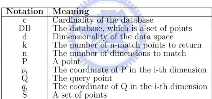
We follow the rules and notations in [21]. Objects from database are considered as multi-dimensional points. We will use object and point interchangeably in the rest of the thesis. Database is considered as a set of d-dimensional points, where d the dimensionality. The notations are shown in Table 1 as follows.

Notation Meaning

c Cardinality of the database

DB The database, which is a set of points d Dimensionality of the data space

k The number of n-match points to return n The number of dimensions to match

P A point

pi The coordinate of P in the i-th dimension

Q The query point

qi The coordinate of Q in the i-th dimension

S A set of points

Table 2.1: Notation

DEFINITION 1. N-match difference

P (p1, p2, ..., pd) and Q(q1, q2, ..., qd) are two d-dimensional points. Let δi = |pi− qi|, i = 1, ..., d.

Sort {δ1, δ2, ..., δd} in increasing order and let sorted array be {δ10, δ02, ..., δd0}. Therefore, the

n-match difference of point P with respect to point Q is δ0 n.

DEFINITION 2. The n-match query

Given a set of d-dimensional points in DB and a n-match query < Q, n > where Q is a query point and n is an integer (1 ≤ n ≤ d), the n-match problem is to search the point P ∈ DB which has smallest n-match difference with respect to Q. P is called n-match point of Q. We use an example shown in Figure 2.1 to describe n-match more specifically. Figure 2.1

(14)

shows a two dimensional space with four points A(1, 3), B(2, 2), C(3, 6),and D(4, 4).Consider the query < Q(0, 0), 1 >, the answer is A because A has smallest 1-match difference (δx = 1)

with respect to Q. When we adjust n to 2, point B becomes the answer because it has smallest 2-match difference (δx = δy = 2) with respect to Q.

D(4,4) C(3,6) B(2,2) A(1,3) Q(0,0) Y -A x is X-Axis

Figure 2.1: The n-match problem

DEFINITION 3. The k-n-match query

Given a set of d-dimensional points in DB of cardinality c, and a k-n-match query < Q, n, k > where Q is a query point, n is an integer (1 ≤ n ≤ d), and k is an integer (k ≤ c), the k-n-match problem is to search k points from DB such that n-k-n-match difference of these k points are less than or equal to the other points in DB.

After giving the definition of the k-n-match query, we know that we can get different set of points with different n. However, it is difficult to determine the value of n in various applica-tions. Instead of determining a value for n, we try different values of n and find k points that appear in answers most frequently. The definition of frequent k-n-match problem is as follows.

DEFINITION 4. The frequent k-n-match query

Given a set of d-dimensional point in DB of cardinality c, and a frequent k-n-match query

< Q, [n0, n1], k > where Q is a query point, [n0, n1] is an interval within [0, d], and k is

an integer (k ≤ c), let S0, ..., Si be the answer sets of k − n0 − match, ..., k − n1 − match,

respectively. Find a set T of k points, so that for any point P1 ∈ T and any point P2 ∈ DB−T ,

P1’s number of appearances in S0, ..., Si is larger than or equal to P2’s number appearances in

S0, ..., Si.

(15)

will compare points only in few features. It is hard to determine if the given points is similar to query point by those few features. On the other hand, frequent k-n-match spend much time on finding answers when we set the interval too large. It will encounter dimensionality problem which have been addressed in [5]. Therefore, we should adjust the interval to get the appropriate answers.

2.2.2 Algorithm AD

To solve k-n-match problem efficiently, the AD algorithm for k-n-match search (KNMatchAD) has been proposed to minimize the number of attribute retrieved. The AD algorithm will access the attributes in Ascending order of their Differences to the query point’s attributes. The AD algorithm for k-n-match search uses some data structures to maintain the necessary information while processing a query. appear[i] maintains the number of appearances of point i. h maintains the number of point ID’s that have appeared n times. S is the answer set. We use the following example to illustrate how algorithm KNMatchAD processes a k-n-match query. Consider the database shown in Table 2.2. Suppose an user requests a query

< Q(3.0, 4.5, 5.5), 2, 2 >. In this case, k=n=2. After sorting attributes of every point in every

dimension, we calculate attribute differences between data points and query point in each dimension and then have sorted lists of difference shown in Figure 2.2. The KNMatchAD will perform as follows: object ID d1 d2 d3 1 0.5 3.0 4.0 2 2.5 5.2 3.0 3 3.3 4.0 7.5 4 6.0 6.5 6.0 5 8.0 9.0 10.0

Table 2.2: An Example Database

Round 1: Locate query values in every dimension. q1(3.0) is located between (2, 2.5) and (3,

3.3); q2(4.5) is located between (3, 4.0) and (2, 5.2); q3(5.5) is located between (1, 4.0) and

(5, 6.0).

Round 2: Find the smallest difference between attribute and qi in every dimension using

binary search toward bigger or smaller attribute directions and store in g[]. g[] has six triples which are {(2,0,0.5) ,(3,1,0.3) ,(3,2,0.5) ,(2,3,0.7) ,(1,4,1.5) ,(4,5,0.5)}.

Round 3: Get the triple (3, 1, 0.3) with smallest dif popped from g[] and appear[3] is increased by 1. Find next smaller difference in dimension 1 towards bigger attribute direction, that is, (4, 6.0), and insert the triple (4, 1, 3.0) into g[1].

(16)

(5,4.0) (4,3.0) (5,4.5) (5,4.5) (2,2.5) (4,2.0) (3,2.0) (1,2.5) (1,1.5) (1,1.5) (2,0.7) (4,0.5) (3,0.5) (2,0.5) (3,0.3) d2 d3 d1

Figure 2.2: Sorted lists of differences

Round 4: Get the triple (2, 0, 0.5) with smallest dif and appear[2] is increased by 1. Find next smaller difference in dimension 1 towards smaller attribute direction, that is, (1, 0.5) and insert the triple (1, 0, 2.5) into g[0].

Round 5: Get the triple (3, 2, 0.5) with smallest dif and appear[3] is increased by 1 and equals 2. appear[3] equals n and h is increased by 1. Find next smaller difference in dimension 2 towards smaller attribute direction, that is, (1, 3.0) and insert triple (1, 2, 1.5) into g[2].

Round 6 and 7 work in a similar way to round 3-5 and h equals k after round 7. Then we can stop KNMatchAD and return S as the answer. Table 2.3 shows the data structures in every round during processing the given k-n-match query.

(a) Round 3 appear {0,0,1,0,0} gd {(2,0.5),(4,3.0),(3,0.5),(2,0.7),(1.,1.5),(4,0.5)} S {} h 0 (b) Round 4 appear {0,1,1,0,0} gd {(1,2.5),(4,3.0),(3,0.5),(2,0.7),(1.,1.5),(4,0.5)} S {} h 0 (c) Round 5 appear {0,1,2,0,0} gd {(1,2.5),(4,3.0),(1,1.5),(2,0.7),(1.,1.5),(4,0.5)} S {3} h 1 (d) Round 6 appear {0,1,2,1,0} gd {(1,2.5),(4,3.0),(1,1.5),(2,0.7),(1.,1.5),(3,2.0)} S {3} h 1 (e) Round 7 appear {0,2,2,1,0} gd {(1,2.5),(4,3.0),(1,1.5),(4,2.0),(1.,1.5),(3,2.0)} S {2,3} h 2

Table 2.3: Structures when processing k-n match query

The AD algorithm for frequent match search (FKNMatchAD) is similar as for k-n-match search. The difference is that frequent k-n-k-n-match search has to monitor number of ap-pearances of points in the interval [n0, n1] given by frequent k-n match query < Q, [n0, n1], k >.

In addition, data structures h[] and S[] displace h and S to maintain appearances of points and answers. In the procedure of FKNMatchAD, if appear[i] is within [n0, n1] , point i will

(17)

equals k. Finally, FKNMatchAD scans S[] to obtain the k point ID’s that appear most times. The detailed steps of FKNMatchAD are described in Algorithm 1.

Algorithm 1: FKNMatchAD

1: Initialize appear[], h[], S[] 2: for every dimension i do 3: Locate qi in dimension i.

4: Calculate the differences between qi and its closest attributes in

dimension i along both directions. Form a triple (pid,pd,dif) for each direction. Put this triple to g[pd].

5: do 6: (pid,pd,dif) = smallest(g); 7: appear[pid]++; 8: if n0 ≤ appear[pid] ≤ n1 then 9: if h[appear[pid] < k then 10: h[appear[pid]]++;

11: S[appear[pid]] = S[appear[pid]] ∪ pid;

12: Read next attribute from dimension pd and form a new triple (pid,pd,dif).

If end of the dimension is reached, let dif be ∞. Put the triple to g[pd].

13: while h[n1] < k

14: scan the top k elements of Sn0, ..., Sn1 to obtain the k point ID’s that appear most

(18)

Chapter 3 Algorithm

3.1 Overview

In this section, we propose an algorithm called CFKNMatchAD to process continuous k-n-match search. CFKNMatchAD is based on AD algorithm for frequent k-n-k-n-match search. Continuous query, unlike traditional query, requires constant evaluation and update when contents of database change. These queries are usually inherently dynamic and related to temporal context. Some changes will not affect the answer. For this reason, we do not have to perform whole procedure of algorithm to check whether the answer changes when data streams fluctuate. Therefore, we do some modification to FKNMatchAD and add it into CFKNMatchAD. We also calculate the intervals called safe region for all attributes of points. Attributes of points can fluctuate within safe regions without changing the answer. Such approach, therefore, can reduce the cost of evaluation for similarity search.

There are two types of continuous query: event-based and time-based. For event-based continuous queries, we report the valid top-k points for the queries after a attribute of point fluctuates. Report operation is driven by attribute-fluctuated event. For time-based continu-ous query, client will give a report period. We find valid top-k points for the query and report them after every report period. Report operation is driven periodically. Our algorithm can be applied to both of continuous queries.

Since our algorithm sets safe region for attributes, we can determine whether the answer may change by safe region and reduce computation without doing unnecessary evaluations. We further classify safe region into two levels. Fluctuated attribute within level one safe region(SR1) will not change the appear[] while fluctuated attribute within level two safe

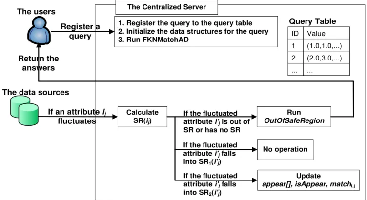
region(SR2) may change appear[]. The procedure of CFKNMatchAD is shown in Figure 3.1.

(19)

1. Register the query to the query table 2. Initialize the data structures for the query 3. Run FKNMatchAD

Query Table

Calculate SR(ij)

Update

appear[], isAppear, matchi,j

Run OutOfSafeRegion No operation Register a query Return the answers If an attribute ij fluctuates If the fluctuated attribute i'j falls into SR1(i'j)

If the fluctuated attribute i'j falls into SR2(i'j)

If the fluctuated attribute i'j is out of SR or has no SR The Centralized Server

The data sources The users ID 1 2 ... Value (1.0,1.0,...) (2.0,3.0,...) ...

Figure 3.1: Procedure of CFKNMatchAD

query table, initialize the data structures for the queries, and run FKNMatchAD to report the first-time answers. Afterward, when the data sources report that an attributes fluctuates, we check where the attribute is. If the attribute falls into its SR1, we do nothing. If the

the attribute falls into its SR2, we update some data structures. If the attribute is out of its

SR or has no safe region, we will run the algorithm called OutOfSafeRegion to obtain valid

answers and report to the users.

To calculate safe region, we use some new data structures as follows.

1.

isAppear

i,j

:

record whether point i in dimension j contributes one match between

i and query point. In other words, isAppeari,j checks if attribute ij makes appear[i]

increase one. In FKNMatchAD, point i will be added to Snif it has n matches between

query point and itself. isAppeari,j is set to false initially. When the triple(pid, pd, dif )

with smallest dif is popped from g[], we set isAppearpid,pd to true.

2.

match

_i,j

:

we set matchi,j to m if attribute ij contributes the m-th match between

point i and query point. For example, we have triple (2,1,0.5) popped form g[] and

appear[2] increases by 1 and equals 2. Then point 2 has 2 matches with respect to query

point and we set match2,1 to 2 because attribute of point 2 in dimension 1 contributes

the 2nd match.

(20)

Thus, the differences of the points that in Sn0, ..., Sn1 are not bigger than threhsold.

3.2 Safe Region

In continuous queries, fluctuated attribute within its safe region will not change the final answer S. We further classify safe region into two levels. Fluctuated attribute within level one safe region(SR1) will not change the appear[] while fluctuated attribute within level two safe

region(SR2) may change appear[]. We do not reevaluate FKNMatchAD if fluctuated attribute

is within safe region and update appear[] if fluctuated feature is within SR2. Therefore, SR1

is defined according isAppear and SR2 is defined according to that whether the point I has

chance to affect S. Because the answer S depends on the appearances of the top k elements in

{Sn0...Sn1}, we have to prevent fluctuated attribute from changing the order of the elements

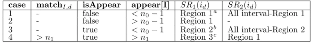
in {Sn0...Sn1} if we want to keep S unchanged. Consider a point I(i0, i2, ..., in) ,we classify

the following cases according to appear[I], isAppearI,d, threshold, matchI,d.

Case 1: If isAppearI,d is false and appear[I] is smaller than n0− 1, this means attribute id

does not contribute any match between I and query point. If still fluctuated attribute i0 ddoes

not contribute any match, S will not change. Hence, we set SR1(id) to [−∞, qd− threshold] ∪

[qd+ threshold, ∞]. Even if i0d contributes a match, appear[I] is smaller than n0 and S will

not change. So we set SR2(id) to all interval - SR1(id).

Case 2: If isAppearI,dis false and appear[I] is bigger than or equals n0−1, this case is similar

to case 1. We set SR1(id) to SR1(id) to [qd− ∞, qd− threshold] ∪ [qd+ threshold, qd+ ∞].

When i0

d contributes a match, this match is possible to become one of {n0...n1}-th match and

may change the element order in the top k positions of {Sn0...Sn1}. Hence, SR2(id) is set to

none.

Case 3: If isAppearI,dis true and appear[I] is smaller than n0− 1, this means idhas already

contributed a match and can not contribute anymore. Then even if i0

dfluctuates to any value,

it will not change S. We set SR1(id) to [qd− tresholdn1, qd+ threshold] and SR2(id) to all

interval - SR1(id).

Case 4: If isAppearI,d is true, appear[I] is bigger than n0 − 1, and matchI,d is bigger than

n1. id contributes the m-th match where m > n1 in this case. Hence, i0d will not change

the element order of the top k positions in {Sn0, ..., Sn1} if |i

0

d− qd| is bigger than |id− qd|.

Hence, we set SR1(id) to [qd− threshold, qd− id] ∪ [qd+ id, qd+ threshold] and SR2(id) to

[qd− ∞, qd− threshold] ∪ [qd+ threshold, qd+ ∞].

(21)

Algorithm 2: CFKNMatchAD

1: FKNMatchAD

2: if attribute id of point I fluctuated with fluctuated attribute i0d then

3: Calculate the safe region for id

4: if i0

d is out of safe region or has no safe region then

5: OutOfSafeRegion()

6: else if id is within SR2 then

7: if isAppearI,d is false then

8: if appear[I] < n0− 1 then

9: appear + +

10: isAppearI,d ← true

11: else

12: if (appear[I] < n0− 1) or (appear[I] > n1 and matchI,d> n1) then

13: appear[I] − −

14: isAppearI,d ← f alse

15: while h[n1] < k do

16: (pid,pd,dif) = smallest(g);

17: appear[pid]++;

18: isAppearpid,pd← true;

19: matchpid,pd ← appear[pid]

20: if n0 ≤ appear[pid] ≤ n1 then

21: h[appear[pid]]++;

22: S[appear[pid]] = S[appear[pid]] ∪ pid;

23: threshold ← dif

24: Read next attribute from dimension pd and form a new triple (pid,pd,dif).

If end of the dimension is reached, let dif be ∞. Put the triple to g[pd].

25: scan the top k elements of Sn0, ..., Sn1 to obtain the k point ID’s that appear most

times

Algorithm 3: OutOfSafeRegion

1: if isAppearI,d is true and |qd− i0d| > threshold and matchI,d= appear[I] then

2: delete I from S[appear[I]]

3: appear[I] − −

4: isAppearI,d ← f alse

5: matchI,d← 0

6: else

7: Reset appear[], h[], isAppear, match, S[]

8: Calculate the differences between qi and its closest attributes in

dimension i along both directions. Form a triple (pid,pd,dif) for each direction. Put this triple to g[pd].

(22)

case matchI,d isAppear appear[I] SR1(id) SR2(id)

1 - false < n0− 1 Region 1a All interval-Region 1

2 - false > n0− 1 Region 1

-3 - true < n0− 1 Region 2b All interval-Region 2

4 > n1 true > n1 Region 3c Region 1

a_{Region 1 is [−∞, q} d− threshold] ∪ [qd+ threshold, ∞] b_{Region 2 is [q} d− tresholdn1, qd+ threshold] c_{Region 3 is [q} d− threshold, qd− id] ∪ [qd+ id, qd+ threshold]

Table 3.1: Safe Region for attribute id of point I

In FKNMatchAD, once the attributes fluctuated, we have to re-sort all of attribute and reevaluate the query. In CFKNMatchAD, if attributes of point i0

d fluctuate, we have to sort

i0

d and place it in right order. But in the case 3, 4, and 5 of CFKNMatchAD mentioned

above, if fluctuated attribute i0

d is within SR1 and isAppearI,d is true, we do not have to sort

i0

d because i0d still contributes a match and do not change the order of points in S[]. Hence,

CFKNMatchAD can save the computation on sorting fluctuated attributes.

The procedure of continuous frequent-k-n-match algorithm (CFKNMatchAD) is shown in Algorithm 2. When a continuous frequent k-n-match query requests, we firstly perform FKNMatchAD and return S. Consider the point I(i1, i2, ..., in). When attribute idis changed,

calculate the safe region defined in Table 3.1. If fluctuated attribute i0

dis out of the safe region,

we perform OutOfSafeRegion shown in Algorithm 3. In algorithm OutOfSafeRegion, we check two conditions that may change S. 1)isAppearI,d is true, |qd− i0d| is bigger than threshold

and matchI,d= appear[I]. In this case, id contributes the largest match between I and query

point, but i0

ddoes not. After idfluctuates, i0d makes I out of Sappear[I]. Hence, we delete I from

Sappear[I] and decrease appear[I] by 1. During the procedure of FKNMatchAD, we add points

into S[] according to similarity order, that is, points in the top position have more similarity to query point. After we delete I from Sappear[I], its position will be replaced immediately by

the point after it in Sappear[I]. The rest part of CFKNMathAD will check the size of Sn1 to

determine if we have to perform FKNMatchAD. Then we just have to scan the points at the top k positions of S[] to obtain the k point ID’s that appear most times. 2) All the other case have to perform FKNMatchAD from initial state because fluctuated attribute may disorder the sequences of elements in {Sn0, ..., Sn1}. Hence, we initialize appear[], h[], isAppear, match

,threshold, and S[] and perform the FKNMatchAD at the end of CFKNMatchAD to get the correct answer S.

On the other hand, we also check fluctuated attribute that within SR2. Fluctuated

at-tribute within SR2 will not change S, but appear[] may need to update. The procedure of

(23)

FKNMatchAD again to check if Sn1 get the top k points.

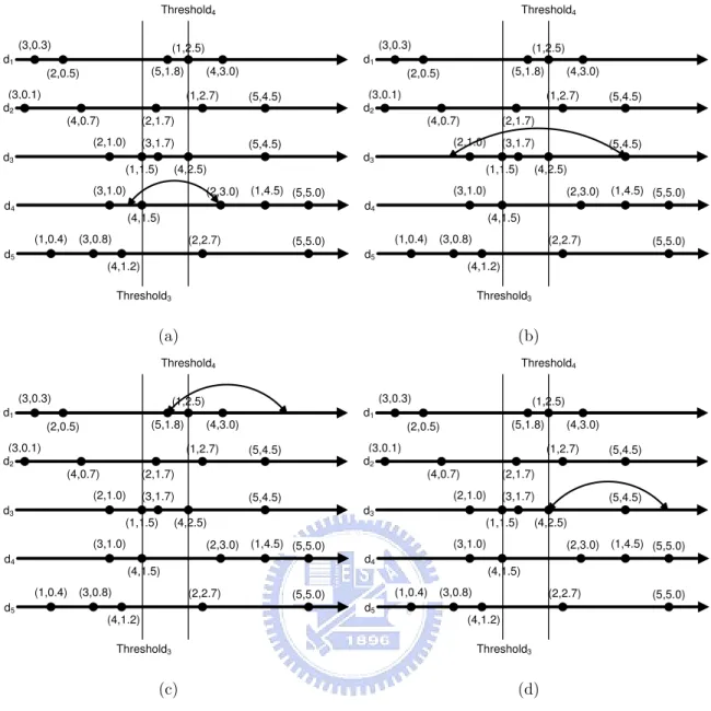
3.3 Running Examples

We take the database shown in Table 3.2 as an example. User requests a query <Q(3.0, 4.5, 5.5, 6.0, 3.5), [3,4], 2>. First, we perform FKNMatchAD and return S. The data structures we need are shown in Table 3.3.

Consider the example shown in Figure 3.2 (a). Suppose that the attribute of point 2 in d4

becomes 7.2 from 9.0. The difference of point 2 in d4 becomes 1.2 from 3.0. It matches case 2 in

Table 3.1 and is out of safe region because |6.0 − 7.2| is smaller than 2.5 (threshold). Because the fluctuated attribute (7.2) of point 2 will make point 4 become out of S3, S will finally

become {2,3}. So it matches the second condition in line 7 in algorithm OutOfSafeRegion and we initialize all the data structures and perform FKNMatchAD to obtain S0_{{2, 3} which}

is different S{2, 4}. Consider the example in Figure 3.2 (b). The attribute of point 5 in d3

becomes 5.3 from 9.0. This matches case 1 in Table 3.1 and the fluctuated attribute (5.3) falls into SR2. Then we update appear[5] to 1. S is still unchanged. Consider the example

in Figure 3.2 (c). The attribute of point 5 in d1 becomes 7.8 from 5.3. This case matches

the case 3 in Table 3.1 and the fluctuated attribute (7.8) falls into its SR2. Then appear[5]

is updated to 0. S does not change. In the example shown in Figure 3.2 (d), the attribute of point 4 in d3 becomes 10.5 from 3.0. The fluctuated attribute has no safe region and matches

the first condition in line 1 in algorithm OutOfSafeRegion. Then we delete point 4 from S4

and S4 has only one element in it. So we perform FKNMatchAD to find the rest element in

S4 and scan S[] to get k points that appear most times.

ID d1 d2 d3 d4 d5 1 0.5 1.8 4.0 1.5 3.1 2 2.5 6.2 6.5 9.0 6.2 3 3.3 4.4 7.2 7.0 4.3 4 6.0 5.2 3.0 4.5 2.3 5 4.8 9.0 10.0 11.0 8.5 Query 3.0 4.5 5.5 6.0 3.5

Table 3.2: An Example for CFKNMatchAD

appear[] {3,3,4,4,1}

S3 {3,4,2,1}

S4 {3,4}

S {3,4}

threshold 2.5

Table 3.3: Structures after performing FKN-MatchAD

THEOREM 3.1. Correctness of CKMatchAD

The points return by algorithm CKNMatchAD compose the k-n-match set of query point Q. PROOF. First, we perform CKNMatchAD to find frequent k-n-match answer sets of query point Q. Every attribute idthat contributes a match is within the interval [qd−threshold, qd+

(24)

Threshold3 Threshold4 (5,1.8) (4,3.0) (5,4.5) (5,4.5) (3,1.7) (2,1.7) (1,1.5) (1,2.5) (2,1.0) (1,2.7) (4,0.7) (4,2.5) (3,0.1) (2,0.5) (3,0.3) d2 d3 d1 (5,5.0) (2,3.0) (4,1.5) (3,1.0) (1,4.5) d4 (5,5.0) (2,2.7) (4,1.2) (3,0.8) (1,0.4) d5 (a) Threshold3 Threshold4 (5,1.8) (4,3.0) (5,4.5) (5,4.5) (3,1.7) (2,1.7) (1,1.5) (1,2.5) (2,1.0) (1,2.7) (4,0.7) (4,2.5) (3,0.1) (2,0.5) (3,0.3) d2 d3 d1 (5,5.0) (2,3.0) (4,1.5) (3,1.0) (1,4.5) d4 (5,5.0) (2,2.7) (4,1.2) (3,0.8) (1,0.4) d5 (b) Threshold3 Threshold4 (5,1.8) (4,3.0) (5,4.5) (5,4.5) (3,1.7) (2,1.7) (1,1.5) (1,2.5) (2,1.0) (1,2.7) (4,0.7) (4,2.5) (3,0.1) (2,0.5) (3,0.3) d2 d3 d1 (5,5.0) (2,3.0) (4,1.5) (3,1.0) (1,4.5) d4 (5,5.0) (2,2.7) (4,1.2) (3,0.8) (1,0.4) d5 (c) Threshold3 Threshold4 (5,1.8) (4,3.0) (5,4.5) (5,4.5) (3,1.7) (2,1.7) (1,1.5) (1,2.5) (2,1.0) (1,2.7) (4,0.7) (4,2.5) (3,0.1) (2,0.5) (3,0.3) d2 d3 d1 (5,5.0) (2,3.0) (4,1.5) (3,1.0) (1,4.5) d4 (5,5.0) (2,2.7) (4,1.2) (3,0.8) (1,0.4) d5 (d)

Figure 3.2: Example of CKNMatchAD Problem

Even if fluctuated attribute contributes or loses one match, appear[I] is still smaller than n0.

Hence, Sn0, ..., Sn1 and S are unchanged. In case 2, original attribute id does not contribute

any match because isAppearI,d is false. We set SR1 to the interval (Region 1 in Table 3.1)

which within the fluctuated attribute still contributes no match and will not affect S. In case 4, the attribute idcontributes the m-th match where m is bigger than n1. We set SR1 to keep

fluctuated attribute i0

d from changing the order of the attributes that contribute l-th match

where l is smaller than m. The other cases that are not in Table 3.1 have no safe region. In Algorithm 3, we initialize all the data structures for the cases that have no safe region or the fluctuated attribute is out of safe region. At the end of CFKNMatchAD, we then check the size of S[] to determine if we need to perform FKNMatchAD to get the top k points. 2

(25)

Chapter 4 Discussion

In this section, we will discuss the extensions of CFKNMatchAD. We discuss the problems of using CFKNMatchAD in the centralized and de-centralized environments. In addition, we also discuss the problem of simulation implementation.

4.1 Centralized Environment

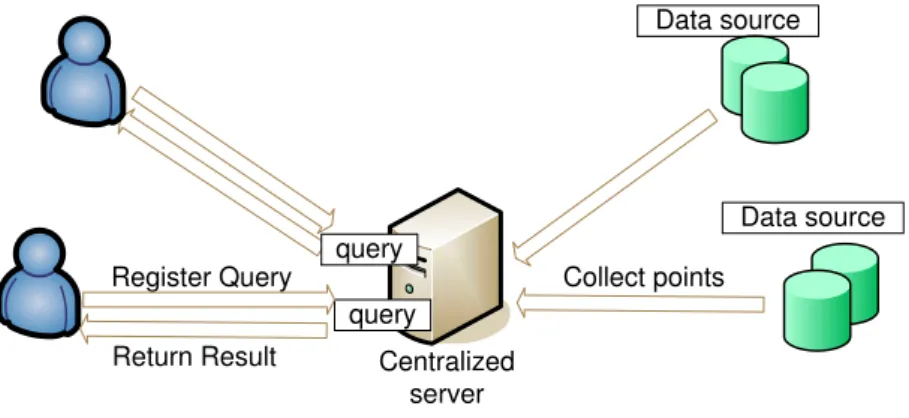
As shown in Figure 4.1, the system for similarity search applications usually has a centralized server with many different data sources. These data sources send data packets that have information about the points to the centralized server. The format of data packet is (id, <

p1, p2, ..., pd >) where id is the point ID and < p1, p2, ..., pd> is the attribute list of the point.

After collecting information of the points, the centralized server receives continuous queries from the clients. Then the centralized server performs CFKNMatchAD and returns S to the clients.

The centralized server reevaluates the queries registered in it and return new top k points after it receives the information about the fluctuated points from the data sources. The Architecture is shown in Figure 4.1. In centralized environment, the data sources will send information of the points to the centralized server and the centralized server checks if it has to reevaluate queries. It is unnecessary that data sources send information of the points to the centralized server if the query results are unchanged.

4.2 Centralized Environment with safe region

To overcome the shortcoming of centralized environment, we do not want the data sources to send unnecessary information to the centralized server if query results will not change.

(26)

Centralized server Return Result

Register Query Collect points query

query

Data source

Figure 4.1: Centralized Environment Architecture

After the centralized server receives continuous queries from clients, it performs first-time CFKNMatchAD and computes safe region for every attribute. Then the centralized server sends safe region of every attribute to the corresponding data sources. The centralized server only send safe region which contains upper and lower bounds to the attribute that contributes a match. For the attribute that do not contribute a match, its difference with respect to the query value is bigger than threshold. So the centralized server only send threshold to those attributes that do not contribute a match. Therefore, every data source can use safe region received from centralized server to check whether fluctuated attributes will change query results. In this environment, the data sources need to have a little computation power to check whether fluctuated attributes are out of safe regions. Only when fluctuated attribute will change query results, the data sources send information of points to inform the centralized server to reevaluate queries. Because of safe region, some fluctuated attribute within its safe region do not sent to the centralized server. Therefore, the centralized server has to send a probe message to all data sources to retrieve all attributes before reevaluating queries. Then the centralized server performs CFKNMatchAD and sends new safe regions to the data sources. By using safe region, unnecessary information can be filtered.

4.3 De-centralized Environment

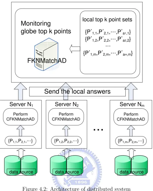
In centralized environment, the centralized server needs to handle all queries from the clients. When there are large volumes queries and points from the clients and data sources respectively, server spends much computation cost on those. If there are other servers that have the same computation power with centralized server, we can use these servers to compute partial answers and send these partial answer to centralized server to compute final answers. By this way, we can decrease the number of points that every server has to handle and balance

(27)

workload of every server. Consider de-centralized environment setting with m + 1 servers:

N1, N2, ..., Nm servers with a centralized server N0. Every server Ni(n < i ≤ m) has data

points {P1,i, P2,i, ..., Pli,i} where liis the number of points in Ni. In de-centralized environment,

when the client registers a frequent k-n-match query < Q, [n0, n1], k > to the N0, N0 gives

every query a unique number qid and broadcasts (qid, < Q, [n0, n1], k >) to every server

Ni(n < i ≤ m). Unlike centralized environment, Ni(n < i ≤ m) does not send information

of the points to the centralized server N0 at first time. According to different query points,

Ni(0 < i ≤ m) performs CFKNMatchAD to find the points that have chance to become final

answers. In traditional similarity search algorithm, a point is determined whether if it is an answer that user wants according a score.

It can be guaranteed that the global top k points are also in the set of the local top k points. However, in frequent k-n match search, an answer point is determined by the number of appearance in Sn0, ..., Sn1. It is possible that a point that is not in the local top k points

is in global Sn0, ..., Sn1. If Ni(0 < i ≤ m) performs CFKNMatchAD to find local top k points

and send them to N0, N0 may lose some points that should be in global Sn0, ..., Sn1. This

problem causes incorrect number of appearance of points in global Sn0, ..., Sn1. To avoid this

problem, we let Ni perform CFKNMatchAD and then send every point {P1,i0 , P2,i0 , ..., Pa0i,i}

that appear in local Sn0, ..., Sn1 and their attributes with corresponding query number qid to

N0 where ai is the number of points in Sn0, ..., Sn1. We will prove that a point that do not

appear in the top k positions of local Sn0, ..., Sn1 will not appear in the top k positions of

global Sn0, ..., Sn1 in the next paragraph. Therefore, we just send the points that appear in

local Sn0, ..., Sn1 and can sure that final answer is correct. Then N0 receives the points from

Ni(0 < i ≤ m) with the same qid and perform FKNMatchAD to find globe top k points.

In Ni(1 < i ≤ m), the attributes of {P1,i, P2,i, ..., Pli,i} have their safe regions. When the

attribute of {P1,i, P2,i, ..., Pli,i} fluctuates, Ni(0 < i ≤ m) performs CFKNMatchAD and then

sends the points that appear in local Sn0, ..., Sn1 to N0 if if the points in local Sn0, ..., Sn1

change. N0 receives the update from Ni(0 < i ≤ m) and performs FKNMatchAD to find new

globe top k points. The architecture of de-centralized environment is shown in Figure 4.2. Proof. In frequent k-n match search, a point that do not appear in the top k position of local Sn0, ..., Sn1 will not appear in the top k position of global Sn0, ..., Sn1.

Let P be a point that do not appear in local Sn0, ..., Sn1. Hence, there are at least k points

that have n-match differences smaller than P where (n0 ≤ n ≤ n1). If we send all points in

local Sn0, ..., Sn1 and P to the centralized server. After performing FKNMatchAD, assume

(28)

Centralized Server N0 {P˅1,1,P˅2,1,Ξ,P˅a1,1} {P˅1,2,P˅2,2,Ξ,P˅a2,2} Ξ {P˅1,m,P˅2,m,Ξ,P˅am,m}

Monitoring

globe top k points

FKNMatchAD

Perform CFKNMatchAD {P1,1,P2,1,Ξ} Perform CFKNMatchAD {P1,2,P2,2,Ξ} Perform CFKNMatchAD {P1,m,P2,m,Ξ} data source

Server N1 Server N2 Server Nm

data source data source

Send the local answers

local top k point sets

Figure 4.2: Architecture of distributed system

differences smaller than P . But we do send all points in local Sn0, ..., Sn1 to the centralized

server. So there are at least k points in global Sn0, ..., Sn1. It contradicts the assumption

and the point P do not exist. Thus, we prove that a point that do not appear in the top k positions of local Sn0, ..., Sn1 will not appear in the top k positions of global Sn0, ..., Sn1. 2

In de-centralized environment, data servers only perform CFKNMatchAD on the points it has and the centralized server only FKNMatchAD on the points received from data servers. Moreover, data servers only send data of the points that appear in the top k positions of local

Sn0, ..., Sn1 to the centralized server. Data servers can eliminate the points that are not the

answers and computation on query process can be balanced by all data servers and response time of each query and network traffic can be reduced. The system we mentioned above are 2-level de-centralized architecture. The data servers are in level 1 and the centralized server is in level 2. To reduce the response time of the queries, we can further deploy more servers to deepen the architecture level. The servers of level 1 are all data servers and the server of top level is the centralized server that is responsible to handle the queries from the clients.

(29)

The servers between level 1 and top level perform FKNMatchAD to find the temporary top k points and send to the server of upper levels.

4.4 Implementation

In continuous queries, the server has to report the valid answer periodically. Therefore, when an attribute fluctuates, we have to check whether the answer is changed and do the reevalua-tion. In every reevalution, FKNMatchAD and CFKNMatchAD have to sort all attributes of the objects in every dimension. This operation cost a lot of computation. Actually, we do not have to sort all attributes and can get the valid answer. After we get the first-time answer, we know how many attributes we retrieve to obtain the valid answer and the differences of these attributes are smaller then threshold. In the next reevaluation, we can only sort the attributes that have differences smaller than threshold plus a value to obtain the valid answer. This will reduce the sorting time significantly and improve the performance of FKNMatchAD and CFKNMatchAD.

(30)

Chapter 5 Performance Evaluation

In this section, we evaluate the efficiency of CFKNMatchAD with different attribute variation rates. We use synthetic data sets generated randomly to run our experiments on a computer with 3.2GHz CPU and 2G RAM.

5.1 Simulation Model

In our simulation model, we use the query and data points with high-dimensional attributes that generated randomly from uniform distribution. First, we generate N data points with

d dimensional attributes data and each normalized attribute is a value within [0,1.0] and is

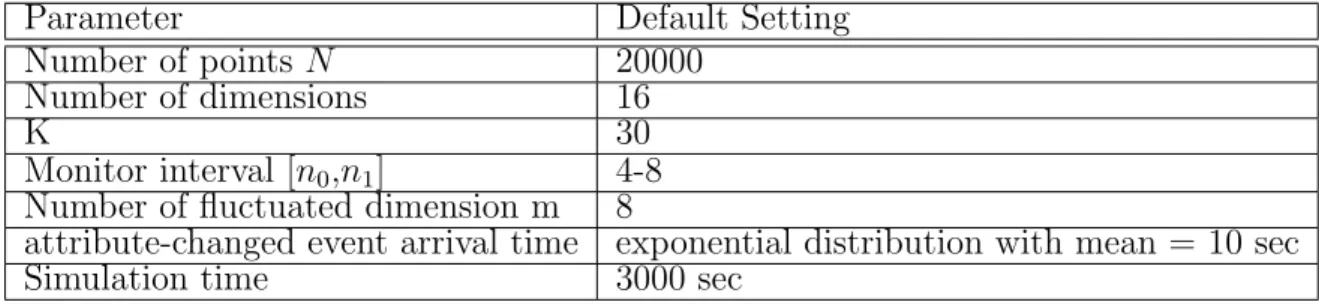
in uniform distribution. We consult [21] to set other system parameters. Table 5.1 lists the default setting of system parameters.

Parameter Default Setting

Number of points N 20000

Number of dimensions 16

K 30

Monitor interval [n0,n1] 4-8

Number of fluctuated dimension m 8

attribute-changed event arrival time exponential distribution with mean = 10 sec

Simulation time 3000 sec

Table 5.1: System Parameters

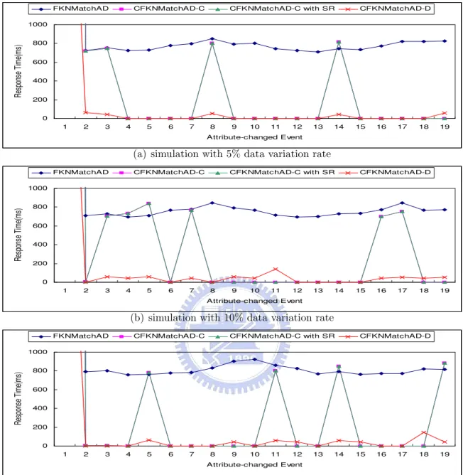
Our experiments compare FKNMatchAD, CFKNMatchAD in centralized environment (CFKNMatchAD-C), CFKNMatchAD in centralized environment with safe region (CFKNMa-tchAD-C with SR) and CFKNMatchAD in de-centralized environment (CFKNMatchAD-D) mentioned in chapter 4. In centralized environment, we have a centralized server received N data points from the data sources. In de-centralized environment, we set 10 servers and a centralized server and assume that N data points are located uniformly in every data server,

(31)

that is, every data server has N/10 data points. The simulation time is 3000 seconds. During simulation, we use exponential distribution to model the interval time that attribute-changed

events arrive and the mean value of distribution is 10 seconds. In every attribute-changed

event, we choose at most m attributes of a random point in different dimensions to fluctuate. After the attribute fluctuates, each approach is performed to find the top k answers and re-port them to the clients. Finally, the average response time of the queries and total network

packet bytes are used as the measurements to compare the performances between four

ap-proaches. Total network packets include point data sent from the data sources to the servers and information of safe region sent from the servers to the data sources. To investigate the impact of safe region, we evaluates the experiments in high, medium, low data variation rates environments. The variation rate is defined as follows.

id− variation rate ≤ i0d ≤ id+ variation rate

Note that the origin attribute is id and fluctuated attribute is i0d. The high, medium, and

low variation rates are 5%, 10%, and 15% respectively. In Figure 5.1, we show the response time of each approach after the first 20 events arrived. The response time of CFKNMatchAD-C and CFKNMatchAD-C with SR are the same because they both are performed in centralized environment. The difference between them is that CFKNMatchAD-C with SR uses safe region to filter unnecessary update packets while CFKNMatch-C does not.

In Figure 5.1, we can see that the response time of FKNMatchAD do reevaluation every time and CFKNMatchAD usually has 0 response time because it uses safe region. Since CFKNMatchAD-D can balance the workload of every processing server and filter some points that will not be the answers, we can see that the response time of CFKNMatchAD-D is significantly lower than the other three approaches. In addition, we can see that first time response times of four approaches are significantly higher. As we mention in chapter 4, in the first time evaluation, we do not know how much attributes we have to retrieve to find the answers. Therefore, we sort all attributes in every dimension. After that, we use the result of the first time evaluation to know how much attributes we retrieve and the differences between query value and those retrieved attributes are smaller than threshold. Therefore, we can only sort the attributes that have differences smaller than threshold plus a value and then we can use these sorted attributes to find the answers. We do not sort all attributes and reduce the sorting time after the first evaluation.

In Figure 5.1, we can see that the fluctuated attributes are out of safe regions more easily in the environment with high data variation rate. Hence, the number of that CFKNMatchAD reevaluates the query increases when the data variation rate increase.

(32)

To analyze the CFKNMatchAD specifically, we classify the average response time into three parts: sorting time, calculating the safe region, and calculating the answers. As Figure 5.2

0 200 400 600 800 1000 1 2 3 4 5 6 7 8 9 10 11 12 13 14 15 16 17 18 19 Attribute-changed Event Re sp on se T im e( m s)

FKNMatchAD CFKNMatchAD-C CFKNMatchAD-C with SR CFKNMatchAD-D

(a) simulation with 5% data variation rate

(b) simulation with 10% data variation rate

(c) simulation with 15% data variation rate

Figure 5.1: Simulation with different data variation rates

˃ ˅˃˃ ˇ˃˃ ˉ˃˃ ˋ˃˃ ˄˃˃˃ ˄ ˅ ˆ ˇ ˈ ˉ ˊ ˋ ˌ ˄˃ ˄˄ ˄˅ ˄ˆ ˄ˇ ˄ˈ ˄ˉ ˄ˊ ˄ˋ ˄ˌ ˅˃ ˔̇̇̅˼˵̈̇˸ˀ˶˻˴́˺˸˷ʳ˘̉˸́̇ ˥˸ ̆̃ ̂́ ̆˸ ʳ˧ ˼̀ ˸ʻ ̀ ̆ʼ ˦̂̅̇˼́˺ ˖˴˿˶̈˿˴̇˼́˺ʳ˦˴˹˸ʳ˥˸˺˼̂́̆ ˖˴˿˶̈˿˴̇˼́˺ʳ˔́̆̊˸̅̆

(33)

shows, the sorting time dominates the average response time. The time using on calculation the safe region and the answers is almost none. Hence, we think that the parameter that affect the sorting time will affect the average response time significantly.

5.2 Impact of point number

In Figure 5.3, we compare the four approaches with 10000-30000 number of points in differ-ent data variation environmdiffer-ents. The Figure 5.3(a)(b)(c) show the results using the average response time as the measurement. In the results, CFKNMatchAD performs better than FKNMatchAD. In different data variation, the total process time of FKNMatchAD are about the same. The response time of all approaches increase when number of points increases. But the response of FKNMatchAD increases more strictly than CFKNMatchAD. Because CFKN-MatchAD does not reevaluate the query after some attribute-changed event arrive, the average response of CFKNMatchAD does not increase as sharp as FKNMatchAD when number of the points increases. In 5.3(d)(e)(f), the experiments use total packet bytes as the measurement. FKNMatchAD and CFKNMatchAD-C have the same number of packet bytes because the data sources report information of all points without filtering any update packets at every attribute-changed event arrives. Contrarily, number of packet bytes of CFKNMatchAD-C with SR and CFKNMatch-D are smaller than the other two approaches. CFKNMatchAD-C with SR uses safe region to filter the unnecessary update packets and CFKNMatchAD-D uses de-centralized architecture to filter the points that will not be in the answer sets. Thus, these two approaches have less number of packet bytes in the simulations. Finally, we can say that CFKNMatchAD has better scalability than FKNMatchAD.

5.3 Impact of dimension number

To examine the scalability of CFKNMatchAD, we also evaluate the experiments with different number of dimension. As shown in Figure 5.4, we evaluate the experiments with 12-20 dimen-sion of point. Since the monitor interval [n0, n1] is fixed, all approaches need to retrieve more

attributes to find the top k answer during processing a query when number of dimension of the point decreases. And threshold also becomes bigger when number of dimension decreases. Because we sort the attributes that have differences smaller than threshold plus a value in every reevaluation, we sort more attributes when threshold becomes bigger. Therefore, the sorting time makes the average response time of all approaches increase when number of

(34)

di-0 500 1000 1500 2000 2500 10000 15000 20000 25000 30000 Number of Points A v e ra g e R e s p o n s e T im e (m s ) FKNMatchAD CFKNMatchAD-C

CFKNMatchAD-C with SR CFKNMatchAd-D

(a) 5% data variation rate

0 500 1000 1500 2000 2500 10000 15000 20000 25000 30000 Number of Points A v e ra g e R e s p o n s e T im e (m s ) FKNMatchAD CFKNMatchAD-C

(b) 10% data variation rate

0 500 1000 1500 2000 2500 10000 15000 20000 25000 30000 Number of Points A v e ra g e R e s p o n s e T im e (m s ) FKNMatchAD CFKNMatchAD-C

(c) 15% data variation rate

0 200000 400000 600000 800000 1000000 1200000 1400000 10000 15000 20000 25000 30000 Number of Points T o ta l P a c k e t B y te s ( FKNMatchAD CFKNMatchAD-C

(d) 5% data variation rate

0 200000 400000 600000 800000 1000000 1200000 1400000 10000 15000 20000 25000 30000 Number of Points T o ta l P a c k e t B y te s (K ) FKNMatchAD CFKNMatchAD-C

(e) 10% data variation rate

0 200000 400000 600000 800000 1000000 1200000 1400000 10000 15000 20000 25000 30000 Number of Points T o ta l P a c k e t B y te s (K ) FKNMatchAD CFKNMatchAD-C

(f) 15% data variation rate

Figure 5.3: Simulation with different number of point

0 200 400 600 800 1000 1200 1400 1600 12 14 16 18 20 Number of Dimensions A v e ra g e R e s p o n s e T im e (m s ) FKNMatchAD CFKNMatchAD-C

0 200000 400000 600000 800000 1000000 1200000 12 14 16 18 20 Number of Dimensions T o ta l P a c k e t B y te s (K ) FKNMatchAD CFKNMatchAD-C

(35)

mension decreases as shown in Figure 5.4(a)(b)(c). In Figure 5.4(d)(e)(f), the results have similar behavior in Figure 5.3(d)(e)(f) because the total packet bytes increase when number of dimension increases.

5.4 Impact of monitor interval [n

0

, n

1

]

In the next simulation, we evaluate every approach under different monitor interval [n0, n1].

In Figure 5.5, we use default value of [n0, n1] and expand n0 and n1 by 1 respectively in zig-zag

manner. Expansion of monitor interval means that we have to monitor additional answer sets and have more points in the answer sets S[]. In Figure 5.5(a)(b)(c), we can see that the average response time of FKNMatchAD increase a little when n0decreases because all approaches only

have to add points to the additional answer sets during the procedure of processing the queries. This does not affect the average response time critically. But the average response time of all approach increase slightly when n0 decreases. If there are more points in the answer sets, we

have higher chance to do the reevaluation because more the attributes are easy to fluctuate out of their safe regions. On the other hand, in Figure 5.5(a)(b)(c), all the average response time increase when n1 increases much because increase of n1. To process a frequent k-n match

query, we have to compute until S[n1] has k points and then find k points that appear most

frequently in S[]. Increase of n1 means that we have to spend more time to find the top

k points and makes the average response time increase. In Figure 5.5(d)(e)(f), we can see that as monitor interval increases, the total packet bytes of CFKMatchAD-C with SR and FKNMatchAD-D also increase and the volume of the increase depends on the increase of the monitor interval but not the value of n0 or n1. But the total packet bytes of FKNMatchAD

and CFKNMatchAD-C are the when monitor interval increases. This is because these the data sources always report information of all points. If number of point and number of dimension do not change, the total packet bytes of these two approaches are the same.

To investigate the impact of n0 and n1 more specifically, we also run the simulations with

different n0 and n1 separately. We set n0 or n1 to the default value and adjust the other one.

The results are shown in Figure 5.6 and 5.7. The increases 5.7(a)(b)(c) are more acute than the increases in In Figure 5.6(a)(b)(c). In Figure 5.6(d)(e)(f) and 5.7(d)(e)(f), we can see that the total packet bytes of CFKNMatchAD-C with SR are affected by the increases of n0 and

(36)

0 500 1000 1500 2000 2500 4~8 3~8 3~9 2~9 2~10 Number of n0-n1 A v e ra g e R e s p o n s e T im e (m s ) FKNMatchAD CFKNMatchAD-C

0 100000 200000 300000 400000 500000 600000 700000 800000 900000 4~8 3~8 3~9 2~9 2~10 Number of n0-n1 T o ta l P a c k e t B y te s (K ) FKNMatchAD CFKNMatchAD-C

Figure 5.5: Simulation with different n0− n1

0 200 400 600 800 1000 1200 2~8 3~8 4~8 5~8 6~8 n0 A v e ra g e R e s p o n s e T im e (m s ) FKNMatchAD CFKNMatchAD-C

0 100000 200000 300000 400000 500000 600000 700000 800000 900000 2~8 3~8 4~8 5~8 6~8 n0 T o ta l P a c k e t B y te s (K ) FKNMatchAD CFKNMatchAD-C

(37)

0 500 1000 1500 2000 2500 4~6 4~7 4~8 4~9 4~10 n1 A v e ra g e R e s p o n s e T im e (m s ) FKNMatchAD CFKNMatchAD-C

Figure 5.7: Simulation with different n1

5.5 Impact of fluctuated dimension number

To measure FKNMatchAD and CFKNMatch in different data variation environment, we not only change data variation rate but also number of fluctuated dimension. Figure 5.8 shows the experiment results with 4-16 fluctuated dimensions. We choose at most 4-16 dimensions to fluctuate in every attribute-changed event. In Figure 5.8(a)(b)(c), the average response time of FKNMatchAD are almost the same because FKNMatchAD reevaluate the queries after every attribute-changed event arrives and number of fluctuated dimension does not affect it. On the other hand, the average response time of CFKNMatchAD increases slightly when number of the fluctuated dimension increases. This is because fluctuation of the attributes in S[] can easily cause reevaluation and number of these attributes are comparatively smaller with respect to the attributes that are not in S[]. Therefore, we think that increase of number of fluctuated dimension dose not cause reevaluation critically. The main reason that affected the performance of CFKNMatchAD is that if the fluctuated attributes are out of their safe regions. In Figure 5.8(d)(e)(f), the results using packet bytes as the measurement have the similar behavior as Figure 5.5(d)(e)(f).

ㄧ個針對連續頻繁之K取N配對搜尋的快速演算法

國

立

交

通

大

學

資訊科學與工程研究所

碩

士

論

文

一 個 針 對 連 續 頻 繁 Ｋ 取 Ｎ 之

配 對 搜 尋 的 快 速 演 算 法

A Fast Algorithm for Continuous Frequent K-N Match

Search

研 究 生：黃壬禾

指導教授：黃俊龍 教授

一個針對連續頻繁之 K 取 N 配對搜尋的快速演算法

A Fast Algorithm for Continuous Frequent K-N Match Search

研 究 生：黃壬禾 Student：Jen-He Huang

指導教授：黃俊龍 Advisor：Jiun-Long Huang

國 立 交 通 大 學

資 訊 科 學 與 工 程 研 究 所

碩 士 論 文

摘

要

在多媒體與資料探勘的應用上，相似度搜尋是一個很重要的議題。目

前大部分的演算法都利用物件的所有特徵來決定彼此之間的相似

度。這些演算法很容易被物件中高差異性的特徵所影響。在 K-N 配對

搜尋中，只將物件的 d 的特徵中取出 k 個來比較，解決的之前演算法

的問題並且能夠有效的找出物件彼此的相似度。在變動的環境中，多

維特徵的資料總是變化地很快。每當資料變化時都重新計算答案很沒

有效率。因此，在這篇論文我們提出了一個針對連續 K-N 配對搜尋的

演算法叫 CFKNMatchAD。我們對每個特徵計算出一個安全領域，只有

當特徵變化跑出安全領域後才會做重新計算的動作，可以大幅節省計

算所花費的消耗並且可以提供正確的答案。實驗的結果我們的演算法

在不同的資料變化率下，可以降低重新計算的花費。另外，CFKNMatch-

AD 還可以應用在分散式環境中來平均計算的花費。

致 謝

首先，我想跟我的家人與朋友分享完成這篇論文的喜悅，感謝他們給

予我的支持，讓我能夠完成這篇論文。我還要感謝我的指導老師黃俊

龍教授，在研究過程中，給予我研究的指導與協助，還有分享他的經

驗，讓我能從不同的觀點來看我的研究。另外，還要感謝實驗的學長

與同學，在跟他們討論中讓我的研究的不足，才能讓這篇論文便的更

完整。最後要感謝他們這兩年的陪伴與鼓勵，讓我的研究生涯中有了

美好的回憶。

Contents

List of Figures

List of Tables

Chapter 1

Introduction

Chapter 2

Preliminaries

2.1

Related Works

2.2

Processing Frequent K-N-Match Queries

2.2.1

Problem definition

2.2.2

Algorithm AD

Chapter 3

Algorithm

3.1

Overview

isAppear

:

match

:

3.2

Safe Region

3.3

Running Examples

Chapter 4

Discussion

4.1

Centralized Environment

4.2

Centralized Environment with safe region

一個針對連續頻繁Ｋ取Ｎ之

配對搜尋的快速演算法

研究生：黃壬禾

指導教授：黃俊龍教授

研究生：黃壬禾 Student：Jen-He Huang

國立交通大學

資訊科學與工程研究所

碩士論文

致謝