Euler’s Graph

Graphs Graphs Graphs

Konigsberg Bridge Problem

• A river Pregel flows around the island Keniphof and then divides into two.

• Four land areas A, B, C, D have this river on their borders.

• The four lands are connected by 7 bridges a – g.

• Determine whether it’s possible to walk across all the bridges exactly once in

returning back to the starting land area.

Konigsberg Bridge Problem (Cont.)

A

Kneiphof

a b

c C d g

D

B f

e

c d

g A e

C

D

Euler’s Graph

• Define the degree of a vertex to be the number of edges incident to it

• Euler showed that there is a walk starting at any vertex, going through each edge

exactly once and terminating at the start vertex iff the degree of each vertex is even. This walk is called Eulerian.

• No Eulerian walk of the Konigsberg bridge problem since all four vertices are of odd edges.

Application of Graphs

• Analysis of electrical circuits

• Finding shortest routes

• Project planning

• Identification of chemical compounds

• Statistical mechanics

• Genertics

• Cybernetics

• Linguistics

• Social Sciences, and so on …

Definition of A Graph

• A graph, G, consists of two sets, V and E.

– V is a finite, nonempty set of vertices.

– E is set of pairs of vertices called edges.

• The vertices of a graph G can be represented as V(G).

• Likewise, the edges of a graph, G, can be represented as E(G).

• Graphs can be either undirected graphs or directed graphs.

• For a undirected graph, a pair of vertices (u, v) or (v, u) represent the same edge.

• For a directed graph, a directed pair <u, v> has u

Three Sample Graphs

0

3

1 2

0

1

3 4

2

5 6

0

1

2

(a) G₁ (b) G₂ (c) G₃

V(G₁) = {0, 1, 2, 3}

E(G₁) = {(0, 1), (0, 2), (0, 3), (1, 2), (1, 3),

V(G₂) = {0, 1, 2, 3, 4, 5, 6}

E(G₂) = {(0, 1), (0, 2), (1, 3), (1, 4),

V(G₃) = {0, 1, 2}

E(G₃) = {<0, 1>,

<1, 0>, <1, 2>}

Graph Restrictions

• A graph may not have an edge from a vertex back to itself.

– (v, v) or <v, v> are called self edge or self loop.

If a graph with self edges, it is called a graph with self edges.

• A graph man not have multiple occurrences of the same edge.

– If without this restriction, it is called a multigraph.

• A simple graph—

– No self-loop

Examples of Graphlike Structures

0

2

1 1

2

3 0

(a) Graph with a self edge (b) Multigraph

Complete Graph

• Each vertex pair has an edge.

• The number of distinct unordered pairs (u, v) with u≠v in a graph with n vertices is

n(n-1)/2.

• A complete unordered graph is an

unordered graph with exactly n(n-1)/2 edges.

• A complete directed graph is a directed graph with exactly n(n-1) edges.

Graph Edges

• If (u, v) is an edge in E(G), vertices u and v are adjacent and the edge (u, v) is the incident on vertices u and v.

• For a directed graph, <u, v> indicates u is adjacent to v and v is adjacent from u.

Subgraph and Path

• Subgraph: A subgraph of G is a graph G’ such that V(G’) V(G) and E(G’) E(G).

• Path: A path from vertex u to vertex v in graph G is a sequence of vertices u, i₁, i₂, …, i_k, v, such

that (u, i₁), (i₁, i₂), …, (i_k, v) are edges in E(G).

– The length of a path is the number of edges on it.

– A simple path is a path in which all vertices except possibly the first and last are distinct.

– A path (0, 1), (1, 3), (3, 2) can be written as 0, 1, 3, 2.

• Cycle: A cycle is a simple path in which the first

⊆

G

and G

Subgraphs

0

3

1 2 0

3

1 2

0

1 2

0 0

1

2

0

1

2

0

1

2 (a) Some subgraphs of G₁

(i) (ii) (iii) (iv)

(i) (ii)

Connected Graph

• Two vertices u and v are connected in an

undirected graph iff there is a path from u to v (and v to u).

• An undirected graph is connected iff for every pair of distinct vertices u and v in V(G) there is a path from u to v in G.

• A connected component of an undirected is a maximal connected subgraph.

• A tree is a connected acyclic graph.

Strongly Connected Graph

• A directed graph G is strongly connected iff for every pair of

distinct vertices u and v in V(G), there is directed path from u to v and also from v to u.

• A strongly connected component is a maximal subgraph that is strongly connected.

Graphs with Two Connected Components

0

3

1 2

0

3

1 2

G₄

H₁ H₂

Strongly Connected Components of G₃

0

1 2

Degree of A Vertex

• Degree of a vertex: The degree of a vertex is the number of edges incident to that vertex.

• If G is a directed graph, then we define

– in-degree of a vertex: is the number of edges for which vertex is the head.

– out-degree of a vertex: is the number of edges for which the vertex is the tail.

• For a graph G with n vertices and e edges, if d_i is the degree of a vertex i in G, then the number of edges of G is

−1 n

Abstract of Data Type Graphs

structure Graph is

objects: a nonempty set of vertices and a set of undirected edges, where each edge is a pair of vertices

functions: for all graph ^∈ Graph, v, v₁ and v₂ ^∈ Vertices Graph Create()::=return an empty graph

Graph InsertVertex(graph, v)::= return a graph with v inserted. v has no incident edge.

Graph InsertEdge(graph, v1,v2)::= return a graph with new edge between v1 and v2

Graph DeleteVertex(graph, v)::= return a graph in which v and all edges incident to it are removed Graph DeleteEdge(graph, v1, v2)::=return a graph in which the edge

(v1, v2) is removed

Boolean IsEmpty(graph)::= if (graph==empty graph) return TRUE else return FALSE

Adjacent Matrix

• Let G(V, E) be a graph with n vertices, n ≥ 1. The adjacency matrix of G is a two-dimensional nxn array, A.

– A[i][j] = 1 iff the edge (i, j) is in E(G).

– The adjacency matrix for a undirected graph is

symmetric, it may not be the case for a directed graph.

• For an undirected graph the degree of any vertex i is its row sum.

• For a directed graph, the row sum is the out- degree and the column sum is the in-degree.

ind vi( ) =

∑

∑

Adjacency Matrices

⎥⎥

⎥⎥

⎦

⎤

⎢⎢

⎢⎢

⎣

⎡

0 1 1 1

1 0 1 1

1 1 0 1

1 1 1 0

3 2 1 0

3 2 1 0

⎥⎥

⎥

⎦

⎤

⎢⎢

⎢

⎣

⎡

0 0 0

1 0 1

0 1 0

2 1 0

2 1 0

⎥⎥

⎥⎥

⎥⎥

⎥⎥

⎥⎥

⎥

⎦

⎤

⎢⎢

⎢⎢

⎢⎢

⎢⎢

⎢⎢

⎢

⎣

⎡

0 1 0 0 0 0 0 0

1 0 1 0 0 0 0 0

0 1 0 1 0 0 0 0

0 0 1 0 0 0 0 0

0 0 0 0 0 1 1 0

0 0 0 0 1 0 0 1

0 0 0 0 1 0 0 1

0 0 0 0 0 1 1 0

7 6 5 4 3 2 1 0

7 6 5 4 3 2 1 0 0

3

1 2

0

1

2

1 0 2

3

4 5

6 7

Adjacency Lists

• Each node in the linked list contains two fields: data and link.

– data: contain the indices of vertices adjacent to a vertex i.

– Each list has a head node.

typedef struct node *node_pointer;

typedef struct node { int vertex;

struct node *link;

};

Adjacent Lists (examples)

3 2 1 0

1 3 3 1

2 0 0 0 0 0 2 0 [0]

[1]

[2]

[3]

0

1 0

2 0 0

[0]

[1]

[2]

HeadNodes HeadNodes

(a) G₁ 0

3

1 2

0

1

Adjacent Lists (example)

2 3 0 1

1 0 0 0 3 0 1 0 [0]

[1]

[2]

[3]

HeadNodes

5 0 6 5 6 0

4 0 7 0 [4]

[5]

[6]

[7]

1 0 2

3

4 5

6

7

Adjacency Lists (cont.)

• The degree of any vertex may be determined by counting the number nodes in its adjacency list.

• The number of edges in G can be determined in O(n + e).

• For a directed graph (also called digraph),

– the out-degree of any vertex can be determined by counting the number of nodes in its adjacency list.

– the in-degree of any vertex can be obtained by keeping another set of lists called inverse

adjacency lists.

Operations for Adjacency Lists

• degree of a vertex in an undirected graph

– Count the number of nodes in its adjacency list

• # of edges in a graph

– Determined in O(n+e)

• out-degree of a vertex in a directed graph

– Count the number of nodes in its adjacency list

• in-degree of a vertex in a directed graph

– Need to traverse the whole data structure – Use inverse adjacency list.

Inverse Adjacency Lists for G₃

1 0

0 0

1 0

[0]

[1]

[2]

0

1

2

Sequential Representation of Graph G₄

9 11 13 15 17 18 20 22 23 2 1 3 0 0 3 1 2 5 6 4 5 7 6

0 1 2 3 4 5 6 7 8 9 10 11 12 13 14 15 16 17 18 19 20 21 22

•Node[i] gives the starting point of the list for vertex i.

•The vertex adjacent from vertex i are stored in

node[node[i]],…,node[node[i+1]].

•For example, node[3] = 15, node[4]=17, so {1, 2} are

adjacent from 3.

1 0 2

3

4 5

6

7

Orthogonal List Representation for G₃

0

1

2 0

1 0 0 0

0 1 0 0

1 2

1 2 0 0 head nodes

(shown twice)

node edge

0

1

2

Multilists

• In the adjacency-list representation of an undirected graph, each edge (u, v) is

represented by two entries.

• Multilists: Nodes in the list are shared among several lists.

– Each edge is represented by one node.

– Each node will be in two lists.

Adjacency Multilists for G₁

[0]

[1]

[2]

[3]

0 1 N1 N3 0 2 N2 N3 0 3 0 N4 1 2 N4 N5 1 3 0 N5 2 3 0 0 N0

N1 N2 N3 N4 N5

HeadNodes

edge (0, 1) edge (0, 2 edge (0, 3) edge (1, 2) edge (1, 3) edge (2, 3) The lists are

Vertex 0: N0 -> N1 -> N2 Vertex 1: N0 -> N3 -> N4 Vertex 2: N1 -> N3 -> N5

0

3

1 2

Graph Operations

• A general operation on a graph G is to visit all vertices in G that are

reachable from a vertex v, that is, all vertices that are connected to v.

– Depth-first search – Breath-first search

Depth-First Search

• Starting from vertex, an unvisited vertex w

adjacent to v is selected and a depth-first search from w is initiated.

• When the search operation has reached a vertex u such that all its adjacent vertices have been

visited, we back up to the last vertex visited that has an unvisited vertex w adjacent to it and

initiate a depth-first search from w again.

• The above process repeats until no unvisited vertex can be reached from any of the visited vertices.

Depth-First Search (recursive algorithm)

void dfs(int v)

{ node_pointer w;

visited[v]= TRUE;

printf(“%5d”, v);

for (w=graph[v]; w; w=w->link) if (!visited[w->vertex])

dfs(w->vertex);

}

Example

0

1 2

7

3 4 5 6

[1]

1 0 0 1 1 2 2 3

0 2 3 5

0 7

0 7

0 7

0 7 4

0 4

0 6

5 6 0

[0]

[2]

[3]

[4]

[5]

[6]

[7

HeadNodes

Depth first search: v0, v1, v3, v7, v4, v5, v2, v6

Analysis of DFS

• If G is represented by its adjacency lists, the DFS time complexity is

O(e). ( e in worst case is n²)

• If G is represented by its adjacency matrix, then the time complexity to complete DFS is O(n²).

Breath-First Search

• Starting from a vertex v, visit all

unvisited vertices adjacent to vertex v.

• Unvisited vertices adjacent to these newly visited vertices are then

visited, and so on.

• If an adjacency matrix is used, the BFS complexity is O(n²).

• If adjacency lists are used, the time complexity of BFS is O(e).

Breath-First Search (algorithm)

void bfs(int v) { node_pointer w;

queue_pointer front, rear;

front = rear = NULL;

printf(“%5d”, v);

visited[v] = TRUE;

addq(&front, &rear, v);

while (front) {

v= deleteq(&front);

for (w=graph[v]; w; w=w->link) if (!visited[w->vertex]) { printf(“%5d”, w->vertex);

addq(&front, &rear, w->vertex);

List ALL Connected Components

void connected(void) { for (i=0; i<n; i++) {

if (!visited[i]) { dfs(i);

printf(“\n”);

} } }

// Complexity?

A Complete Graph and Three of Its Spanning Trees

•A spanning tree is any tree consisting solely of edges in G and including all vertices in G.

Depth-First and Breath-First Spanning Trees

3 4

1 2

5 6

0

7

3 4

1 2

5 6

0

7

(a) DFS (0) spanning tree (b) BFS (0) spanning tree

•Spanning tree can be obtained by using either a depth-first or a breath-first search.

Properties of Spanning Tree

• When a nontree edge (v, w) is introduced into any spanning tree T, a cycle is formed.

• A spanning tree is a minimal subgraph, G’, of G such that V(G’) = V(G), and G’ is

connected. (Minimal subgraph is defined as one with the fewest number of edges).

• Any connected graph with n vertices must have at least n-1 edges, and all connected graphs with n – 1 edges are trees.

Therefore, a spanning tree has n – 1 edges.

Biconnected Components

• Definition: A vertex v of G is an articulation point iff the deletion of v, together with the deletion of all edges incident to v, leaves behind a graph that has at least two connected components.

• Definition: A biconnected graph is a connected graph that has no articulation points.

• Definition: A biconnected component of a connected graph G is a maximal biconnected subgraph H of G. By maximal, we mean that G contains no other subgraph that is both

biconnected and properly contains H.

A Connected Graph and Its Biconnected Components

0

1

4

2 3

8

7

6 5

9

1

4

2 3

7

6 5

0

1

3 5

8

7 7

9

(a) A connected, but

Biconnected Components (Cont.)

• Two biconnected components of the same graph can have at most one vertex in common.

• No edge can be in two or more biconnected components.

• The biconnected components of G partition the edges of G.

• The biconnected components of a connected, undirected graph G can be found by using any depth-first spanning tree of G.

• A nontree edge (u, v) is a back edge with respect to a spanning tree T iff either u is an ancestor of v

Biconnected Components (Cont.)

• The root of the depth-first spanning tree is an articulation point iff it has at least two children.

• Any other vertex u is an articulation point iff it has at least one child, w, such that it is not

possible to reach an ancestor of u using apath composed solely of w, descendants of w, and a single back edge.

• Define low(w) as the lowest depth-first number that can be reached from w using a path of

descendants followed by, at most, one back edge.

}, of

child a

is

| ) ( min{

), ( min{

)

(w dfn w low x x w

low =

Conditions for Articulation point

• u is an articulation point iff u is

either the root of the spanning tree and has two or more children or u is not the root and u has a child w such that low(w) ≥ dfn(u).

Depth-First Spanning Tree

0

1

4

2 3

8

7

6 5

9

1

2 3

4 5

6

7 8 10 9

3

4 2 1 0

6 7 8 5

9

1

2

3

4

5

6

7

8

9 10

dfn and low values for the Spanning Tree

9 10

6 6

6 1

1 1

1 5

low

9 10

8 7

6 2

1 3

4 5

dfn

9 8

7 6

5 4

3 2

1 0

vertex

Weighted Edges

• Very often the edges of a graph have weights associated with them.

– distance from one vertex to another – cost of going from one vertex to an

adjacent vertex.

– To represent weight, we need additional field, weight, in each entry.

– A graph with weighted edges is called a network.

Minimal Cost Spanning Tree

• The cost of a spanning tree of a weighted,

undirected graph is the sum of the costs (weights) of the edges in the spanning tree.

• A minimum-cost spanning tree is a spanning tree of least cost.

• Three greedy-method algorithms available to obtain a minimum-cost spanning tree of a

connected, undirected graph.

– Kruskal’s algorithm – Prim’s algorithm – Sollin’s algorithm

Kruskal’s Algorithm

• Kruskal’s algorithm builds a minimum-cost

spanning tree T by adding edges to T one at a time.

• The algorithm selects the edges for inclusion in T in nondecreasing order of their cost.

• An edge is added to T if it does not form a cycle with the edges that are already in T.

• Theorem 6.1: Let G be any undirected, connected graph. Kruskal’s algorithm generates a minimum- cost spanning tree.

• O(E log E)

Stages in Kruskal’s Algorithm

0

5

1

6

4 3

2

0

5

1

6

4 3

2

10

(a) (b) (c)

0

5

1

6

4 3

2

10

28

14 16

18 12 22

25 24

Stages in Kruskal’s Algorithm (Cont.)

0

5

1

6

4 3

2

10

0

5

1

6

4 3

2

(d) (e) (f)

12

10

12 14

0

5

1

6

4 3

2

10

12

14 16

Stages in Kruskal’s Algorithm (Cont.)

0

5

1

6

4 3

2

10

14 16

12 22

(g)

0

5

1

6

4 3

2

10

14 16

12 22

(g)

25

Kruskal’s Algorithm

T= {};

while (T contains less than n-1 edges && E is not empty) {

choose a least cost edge (v,w) from E;

delete (v,w) from E;

if ((v,w) does not create a cycle in T) add (v,w) to T

else discard (v,w);

}if (T contains fewer than n-1 edges) printf(“No spanning tree\n”);

Prim’s Algorithm

• Similar to Kruskal’s algorithm, Prim’s algorithm

constructs the minimum-cost spanning tree edge by edge.

• The difference:

– the set of selected edges forms a tree at all times when using Prim’s algorithm

– the set of selected edges forms a forest when using Kruskal’s algorithm.

• In Prim’s algorithm, a least-cost edge (u, v) is added to T such that T∪ {(u, v)} is also a tree. This

repeats until T contains n-1 edges.

Prim’s algorithm in program 6.7 has a time

Stages in Prim’s Alogrithm

0

5

1

6

4 3

2

10

0

5

1

6

4 3

2

10

25

0

5

1

6

4 3

2

10

25

22

0

5

1

6

4 3

2

10

28

14 16

18 12 22

25 24

Stages in Prim’s Alogrithm (Cont.)

0

5

1

6

4 3

2

(d)

10

25

22

12

0

5

1

6

4 3

2

(e)

10

25

22

12 16

0

5

1

6

4 3

2

(f)

10

25

22

12 14 16

Prim’s Alogrithm

T={};

TV={0};

while (T contains fewer than n-1 edges) {

let (u,v) be a least cost edge such that if (there is no such edge ) break;and

add v to TV;

add (u,v) to T;

}if (T contains fewer than n-1 edges)

TV u ∈

TV v ∉

Sollin’s Algorithm

• Contrast to Kruskal’s and Prim’s algorithms,

Sollin’s algorithm selects multiple edges at each stage.

• At the beginning, each tree in this forest is a single vertex.

• During each stage, an minimum-cost edge is selected for each tree in the forest.

• It’s possible that two trees in the forest to select the same edge. Only one should be used.

• Also, it’s possible that the graph has multiple edges with the same cost. So, two trees may select two different edges that connect them

Stages in Sollin’s Algorithm

0

5

1

6

4 3

2

10

14

12 22

(a)

25

0

5

1

6

4 3

2

(b)

10

22

12 14 16

0

5

1

6

4 3

2

10

28

14 16

18 12 22

25 24

0

5

1

6 2

Shortest Paths

• Usually, the highway structure can be represented by graphs with vertices

representing cities and edges representing sections of highways.

• Edges may be assigned weights to

represent the distance or the average

driving time between two cities connected by a highway.

• Interested in answers to the following question:

– (1) Is there a path from A to B

– (2) If there is more than one path from A to B, which path is the shortest?

Single Source/All Destinations:

Nonnegative Edge Costs

• Let S denotes the set of vertices to which the shortest paths have already been found.

1) If the next shortest path is to vertex u, then the path begins at v, ends at u, and goes through only vertices that are in S.

2) The destination of the next path generated must be the vertex u that has the minimum distance among all vertices not in S.

3) The vertex u selected in 2) becomes a member of S.

• The algorithm is first given by Edsger Dijkstra.

Therefore, it’s sometimes called Dijstra Algorithm.

) (u ∉ S

Graph and Shortest Paths From Vertex 0 to all destinations

0

3 4

1 2

5

10 20

50

15

20

10

35

30

3 15

Path Length

1) 0, 3 2) 0, 3, 4 3) 0, 3, 4, 1 4) 0, 2

10 25 45 45

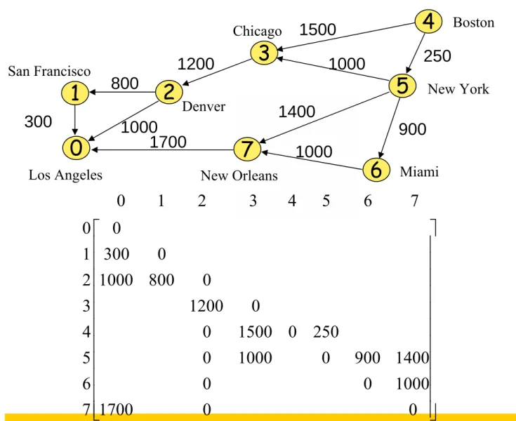
Diagram for Example 6.5

0

1 2

3

4 5

7 6

300

800

10001700

1000 1400 1200

1500

1000 250

900

Los Angeles San Francisco

Denver

New Orleans Miami

New York Boston Chicago

⎥⎥

⎥⎥

⎥⎥

⎥⎤

⎢⎢

⎢⎢

⎢⎢

⎢⎡

250 0

1500 0

0 1200

0 800

1000 0 300

0

4 3 2 1 0

7 6

5 4 3

2 1

0

Dijstra Algorithm

void shortestpath(int v, int cost[][MAX_ERXTICES], int distance[], int n, short int found[])

{

int i, u, w;

for (i=0; i<n; i++) { found[i] = FALSE;

distance[i] = cost[v][i];

}

found[v] = TRUE;

distance[v] = 0;

Dijstra Algorithm (cont.)

for (i=0; i<n-2; i++) {

u = choose(distance, n, found); // select minimum Distance[]

found[u] = TRUE;

for (w=0; w<n; w++) if (!found[w])

if (distance[u]+cost[u][w]<distance[w]) distance[w] = distance[u]+cost[u][w];

} }

4 5 3

1500

250

D[3]=1500, D[5]=250, Others = ∞

(a) (b)

D[3]=1250, D[5]=250, D[6]=1150, D[7]=1650

6

900 5

250

4

7

1000

(c)

6 ⁹⁰⁰ 3

5

1000 250

4

1400

7

1000

(d)

6 ⁹⁰⁰ 3

5

1000 250

4

1400

2 ¹²⁰⁰ 3

1500

7

1400 1000

2

7

1700

(e)

6 ⁹⁰⁰ 3

5

1000 250

4

1400 1200

0

2

7

1700

(g)

6 ⁹⁰⁰ 3

5

1000 250

4

1400 1200

0 1

800 300 1000

D[0]=3350, D[2]=2450, D[3]=1250, D[5]=250, D[6]=1150, D[7]=1650

Action of Shortest Path

{4,5,6,3,7, 2,1}

1650 1150

250 0

1250 2450

3250 3350

1 {4,5,6,3,7,

6 2}

1650 1150

250 0

1250 2450

3250 3350

2 {4,5,6,3,7}

5

1650 1150

250 0

1250 2450

+∞

3350 7

{4,5,6,3}

4

1650 1150

250 0

1250 2450

+∞

+∞

3 {4,5,6}

3

1650 1150

250 0

1250 +∞

+∞

+∞

6 {4,5}

2

1650 1150

250 0

1250 +∞

+∞

+∞

5 {4}

1

+∞

+∞

250 0

1500 +∞

+∞

+∞

--- --

Initial

[7]

[6]

[5]

[4]

[3]

[2]

[1]

[0]

NO MIA

NY BOST

CHI DEN

SF LA

Distance Vertex

selected S

iteration

Directed Graphs

0 1 2

5

7 -5

0 1 2

-2

1 1

(a) Directed graph with a negative-length edge

(b) Directed graph with a cycle of negative length No shortest path

solution

All-Pairs Shortest Paths

• In all-pairs shortest-path problem, we are to find the shortest paths between all

pairs of vertices u and v, u ≠ v.

– Use n independent single-source/all-destination problems using each of the n vertices of G as a source vertex. Its complexity is O(n³)

All-Pairs Shortest Paths (Cont.)

• A^k[i][j]: the length of the shortest path from I to j going through no intermediate vertex of index greater than k.

• A^n-1[i][j]: the length of the shortest i-to-j path in G

• A^-1[i][j]: is just the length[i][j]

• The shortest path goes through vertex k. The path consists of subpath from i to k and another one from k to j

A^k[i][j] = min{A^k-1[i][j], A^k-1[i][k]+ A^k-1[k][j] }, k ≥ 0

All-Pairs Shortest Paths Algorithm

void allcost(int cost[][MAX_VERTICES], int distance[]

[][MAX_VERTICES], int n) { int i, j, k;

for (i=0; i<n; i++)

for (j=0; j<n; j++)

distance[i][j] = cost[i][j];

for (k=0;n k < n; k++) for (i=0; i<n; i++)

for (j=0; j<n; j++)

if (distance[i][k] + distance[k][j] < distance[i][j]) distance[i][j] = distance[i][k]+distance[k][j];

}

Example for All-Pairs Shortest-Paths Problem

0 3 ∞

2

2 0

6 1

11 4

0 0

2 1

0 A^---111

0 7

3 2

2 0

6 1

11 4

0 0

2 1

0 A⁰⁰⁰

0 7

3 2

2 0

6 1

6 4

0 0

2 1

0 A¹¹¹

2

0 1

6

2 4

11 3

0 7

3 2

2 0

5 1

6 4

0 0

2 1

0 A²²²

(b) A^-1 (c) A⁰

Transitive Closure

• Definition: The transitive closure

matrix, denoted A⁺, of a graph G, is a matrix such that A⁺[i][j] = 1 if there is a path of length > 0 fromi to j;

otherwise, A ⁺[i][j] = 0.

• Definition: The reflexive transitive closure matrix, denoted A^*, of a

graph G, is a matrix such that A^*[i][j]

= 1 if there is a path of length 0 from i to j; otherwise, A^*[i][j] = 0.

Transitive Closure Algorithm

void transitive_closure(int cost[][MAX_VERTICES], int distance[] [][MAX_VERTICES], int n) {

int i, j, k;

for (i=0; i<n; i++)

for (j=0; j<n; j++)

distance[i][j] = cost[i][j];

for (k=0;n k < n; k++) for (i=0; i<n; i++)

for (j=0; j<n; j++)

distance[i][j]= distance[i][j] ||

distance[i][k] && distance[k][j];

Graph G and Its Adjacency Matrix A, A⁺, A^*

⎥⎥

⎥⎥

⎥⎥

⎤

⎢⎢

⎢⎢

⎢⎢

⎡

1 1 1 0 0

1 1 1 0 0

1 1 1 0 0

1 1 1 1 0

3 2 1 0

4 3 2 1 0

⎥⎥

⎥⎥

⎥⎥

⎦

⎤

⎢⎢

⎢⎢

⎢⎢

⎣

⎡

0 0 0 0 0

1 0 0 0 0

0 1 0 0 0

0 0 1 0 0

0 0 0 1 0

4 3 2 1 0

4 3 2 1 0

0 1 2 3 4

(a) Digraph G

⎥⎥

⎥⎥

⎤

⎢⎢

⎢⎢

⎡

1 1 1 0 0

1 1 1 0 0

1 1 1 1 0

1 1 1 1 1

3 2 1 0

4 3 2 1 0

(b) Adjacency matrix A

Activity-on-Vertex (AOV) Networks

• Definition: A directed graph G in which the vertices represent tasks or activities and the edges represent precedence relations between tasks is an activity-on-vertex network or AOV network.

• Definition: Vertex i in an AOV network G is a predecessor of vertex j iff there is a directed path from vertex i to vertex j. i is an immediate predecessor of j iff <i, j> is an edge in G. If i is a predecessor of j, then j is an successor of i. If i is an immediate predecessor of j, then j is an immediate

of i.

Activity-on-Vertex (AOV) Networks (Cont.)

• Definition: A relation · is transitive iff it is the

case that for all triples, i, j, k, i.j and j·k => i·k. A relation · is irreflexive on a set S if for no element x in S it is the case that x·x. A precedence

relation that is both transitive and irreflexive is a partial order.

• Definition: A topological order is a linear ordering of the vertices of a graph such that, for any two vertices I and j, if I is a predecessor of j in the network, then i precedes j in the linear ordering.

An Activity-on-Vertex (AOV) Network

C7 Computational Theory

C13

C7 Artificial Intelligence

C12

C10 Compiler Design

C11

C7 Programming Languages

C10

C7, C8 Operating Systems

C9

C3 Assembly Language

C8

C3, C6 Analysis of Algorithms

C7

C5 Linear Algebra

C6

C4 Calculus II

C5

None Calculus I

C4

C1, C2 Data Structures

C3

None Discrete Mathematics

C2

None Programming I

C1

Prerequisites Course name

Course number

An Activity-on-Vertex (AOV) Network (Cont.)

C1

C2

C3 C7

C8

C13 C12 C10 C9

C14 C11 C1, C2, C4, C5, C3, C6, C8,C7, C10, C13, C12, C14,

C15, C11, C9

C4, C5, C2, C1, C6, C3, C8, C15, C7, C9, C10, C11, C13,

C12, C14

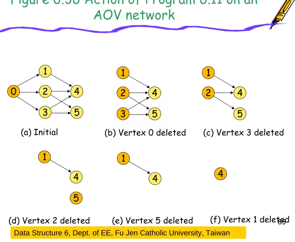
Topological Sort

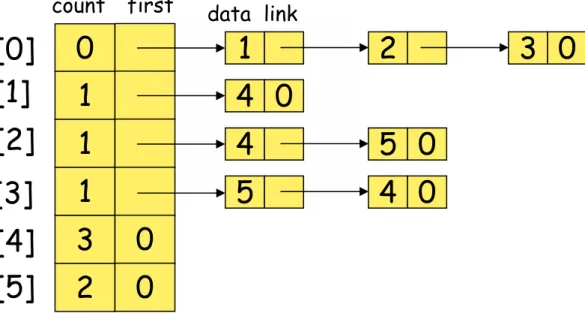
for (i = 0; i < n; i++) {

if every vertex has a predecessor {

fprintf(stderr, “Network has a cycle. \n “ );

exit(1);

}

pick a vertex v that has no predecessors;

output v;

delete v and all edges leading out of v from the network;

}