國立臺灣大學電機資訊學院資訊工程學系 碩士論文
Department of Computer Science and Information Engineering College of Electrical Engineering and Computer Science
National Taiwan University Master Thesis
具時間限制的廣播中心問題
Broadcast Centers in Trees with Time Constraints
黃煜翔 Yu-Shiang Huang 指導教授:陳健輝博士 Advisor: Gen-Huey Chen, Ph.D.
指導教授:林清池博士 Advisor: Ching-Chi Lin, Ph.D.
中華民國 104 年 6 月 June, 2015
誌謝
感謝神明安排我做這個論文題目。
Acknowledgements
I’m glad to thank the god for assigning this problem.
摘要
本論文提出一 O(n)時間複雜度的演算法來解決樹狀結構
上的廣播中心點問題,使廣播中心點的數量最少。廣播 按照異質郵寄模型的規則進行,需在時間限制內完成。
關鍵字: 廣播中心點問題,時間限制,異質郵寄模型,
樹狀結構,貪進法。
Abstract
In this thesis, we present a O(n)-time exact algorithm to find a broadcast strategy such that broadcasting can be completed within the time constraint and the number of centers is mini- mal. The given graph is a tree and broadcasting is under the heterogeneous postal model.
Keywords: broadcast center problem, time constraint, hetero- geneous postal model, trees, greedy method.
Contents
口試委員會審定書 iii
誌謝 v
Acknowledgements vii
摘要 ix
Abstract xi
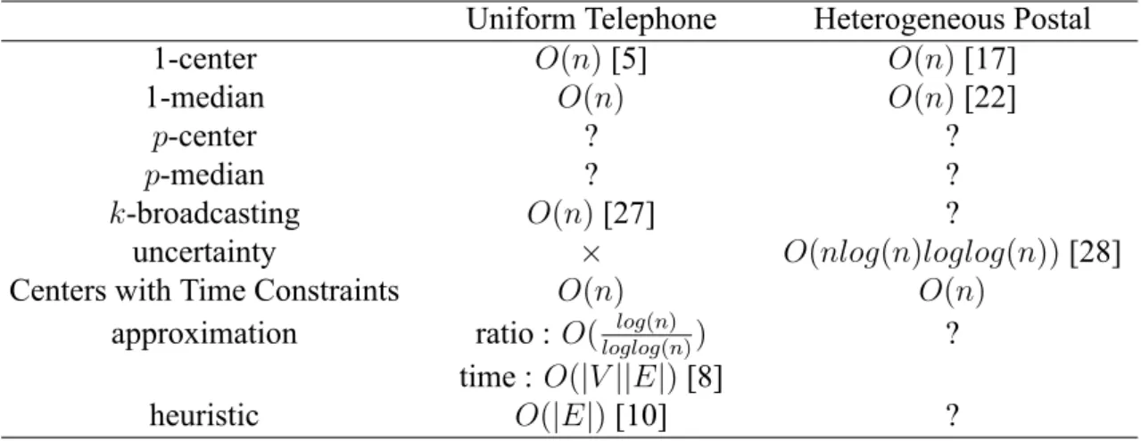
1 Introduction 1
1.1 Broadcast Problem and Models . . . 1 1.2 Main Results and Thesis Organization . . . 2
2 Preliminaries 3
2.1 Notations and Definitions . . . 3 2.2 Related Works . . . 5
3 A Linear-Time Algorithm 7
3.1 Algorithm Description . . . 7 3.2 FindingSU CC(v) and b_time(v) . . . 9 3.3 Evaluatngspare(v) . . . 11
3.4 A Non-Sorting Method . . . 12 3.5 Time Complexity . . . 16
4 Correctness 19
4.1 Minimum Unused Edges and Broadcast Time . . . 20 4.2 Earliest Spare Time . . . 23 4.3 Correctness of the Algorithm . . . 24
5 Two Illustrative Examples 29
5.1 The First Example . . . 29 5.2 The Second Example . . . 39
6 Conclusion 47
Bibliography 49
List of Figures
3.1 Tree T89535. . . 10
3.2 Tree T368. . . 13
3.3 An Example of Reordering. . . 15
5.1 GraphG0. . . 29
5.2 Tree T1. . . 30
5.3 Tree T2. . . 39
List of Tables
1.1 Models . . . 2 3.1 Different broadcast sequences may lead to different broad-
cast time . . . 13 6.1 Broadcast problems in uniform telephone model and het-
erogeneous postal model . . . 47
Chapter 1 Introduction
Broadcasting is an important problem in our life; the main objective is finding efficient strategies to deliver the messages. In many distributed or point-to-point systems, like people and mobile devices in a crowded place, every node can only contact with nodes nearby. Broadcasting makes every node in the system reveived the message.
1.1 Broadcast Problem and Models
Broadcastingis an information dissemination problem. In a graph net- work G(V, E), there are at least one broadcast center, which has the message before broadcasting starts. During broadcasting, nodes have the message can set up calls, which copy the message to their neigh- bors. A call fromuto vis made up of two phases. The first one issetup phase; it takesα time. During setting up,ucannot do other things. The other one is transmission phase; it takesw(u, v) time. Node ucan set up a connection to another node, while transmitting messages to node v. Under these conditions, the time and the distances may affect our broadcasting strategies.
Thebroadcast centers with time constraints problem is defined as below. Given Given a graphG(V, E)and a time constraintt, the broad-
cast centers with time constraints problem is to determine OP T (G, t), the minimal number of centers required.
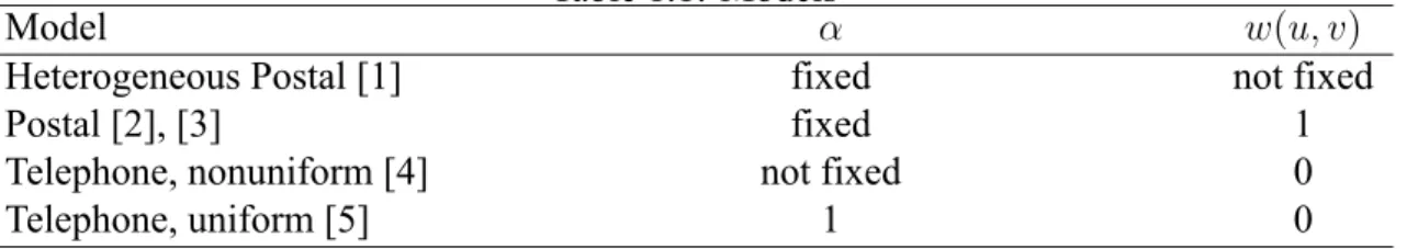
There are several models in broadcasting problem. The uniform tele- phone model is the first introduced model; it is also the most widely- studied model. Under the nonuniform telephone model, the setup time, α, from u to v, is the length of the edge (u, v). Under the heteroge- neous postal model, the setup time,α, is a non-negative number, and the transmission time,w(u, v), is the length of the edge(u, v). This compar- ison tells us both the uniform telephone model and the postal model are special cases of the heterogeneous postal model. In other words, once problems under the heterogeneous postal model are solved, the same problems under the uniform telephone model is also solved. Table 1.1 lists several models.
Table 1.1: Models
Model α w(u, v)
Heterogeneous Postal [1] fixed not fixed
Postal [2], [3] fixed 1
Telephone, nonuniform [4] not fixed 0
Telephone, uniform [5] 1 0
1.2 Main Results and Thesis Organization
We propose an O(n)-time deterministic algorithm to solve the broad- cast centers with time constraints problem on trees under heterogeneous postal model.
Chapter 2 presents many notations and definitions we will use. Chap- ter 3 presents the algorithm and its time complexity. Chapter 4 shows the correctness of the algorithm. Chapter 5 presents execution of the algorithm with two examples.
Chapter 2
Preliminaries
We use a graph to represent a network. Before introducing the algorithm, we introduce several notations, definitions, and related problems.
2.1 Notations and Definitions
A graph is made up of nodes and edges. We use G(V, E)to represent a graph, where V is the set of nodes and E is the set of edges. An edge is a curve connects two endpoints. We use (u, v) to represent an edge where u and v are its two endpoints; we denote w(u, v) as its length.
An another graph G′(V′, E′) is said a subgraph of G iff V′ ⊆ V and E′ = {(u, v) ∈ E|u, v ∈ V′}. A node u is a neighbor of v iff there is an edge(u, v) in G. We use N (v) to represent the set of neighbors of v. The degree of a node v is the number of edges where v is an endpoint.
In this thesis, without mentioned particularly, every graph is undirected and simple. Simple means there are no (v, v), edges such that its two endpoints are identical and there is at most one edge for every node pair.
A sequence of edges is a walk if this sequence has the form
((u0, u1), (u1, u2),· · · , (uk−1, uk)). If u0, u1,· · · , uk are distinct, it is a
path; if they are distinct except u0 = uk, it is a cycle. A graph is con- nected if for every couple of nodes uand v, there is a path from uto v. A tree is a connected graph without cycles. A tree T is a spanning tree of a graphGif T can be obtained by removing edges from G.
After the basic knowledges are introduced, we introduce several terms we will use in this thesis. Let (u, v) be an edge in T. Removing (u, v) from T leads to two trees, T (u, v) and T (v, u) where T (u, v) contains u and T (v, u) contains v. The predecessor of v, pred(v), is a neighbor ofv such thatv receives the message from pred(v) when broadcasting.
We use pred(v) = ∅ to represent v has no predecessor. The successors of v, SU CC(V ), is an ordered subset of the neighbors of v. A vertex u ∈ SUCC(v)ifu receives the message fromv when broadcasting.
The broadcast time of v,b_time(v, S), is the time required to broad- cast a message from v to all nodes in ∪
x∈ST (x, v). The default value ofS isSU CC(v); that is,b_time(v) = b_time(v, SU CC(v)).
b_time(v) =
0, ifSU CC(v) = ∅;
max{iα + w(v, ui) + t(ui)|1 ≤ i ≤ k},
ifSU CC(v) = (u1, u2,· · · , uk).
The successor candidates of v, SU CC∗(v), is a subset of previously processed neighbors of v. A vertex u ∈ SUCC∗(v), if pred(u) = ∅ and α + w(v, u) + b_time(u) ≤ t. The predecessor candidates of v, P RED∗(v), is a subset of previously processed neighbors ofv. A vertex u ∈ P RED∗(v), ifu /∈ SUCC(v) and spare(u) + α + w(v, u)≤ t.
The arrive time ofv,arrive(v), is the earliest time v knows the mes- sage. The earliest spare time of v, spare(v), is the earliest time that v can set up a connection with a receiver u /∈ SUCC(v) under the con- straint that the broadcasting from v to the subtrees rooted by nodes on SU CC(v) can still be completed in t. The unused edges of T, E−(T ), is a subset of E(T ). An edge (u, v) ∈ E−(T ) iff u ̸= pred(v) and v ̸= pred(u). We use E− = E−(T ) where T is the input tree. We use E−(v) = E−(N [v]).
2.2 Related Works
The broadcasting problem has been studied for several decades. It was firstly introduced by Slateret al. [5]; they proved that both finding the optimal broadcast center and finding the minimum broadcast time on general graphs are NP-complete. They also proposed a linear-time al- gorithm for finding the optimal broadcast center and minimum broadcast time on trees under the uniformed telephone model.
There are approximation algorithms proposed for finding the mini- mum broadcast time. An O(loglog(n)log2(n) )-approximate algorithm was pre- sented in [6], where n is the number of vertices. An O(√
n)-additive- approximate algorithm was presented in [7]. Also, there are approxima- tion algorithms for finding the minimum multicast time from a vertex to a subset of k vertices. An O(loglog(k)log(n) )-approximate algorithm was presented in [1]; an O(loglog(k)log(k) )-approximate algorithm was presented in [8]. Besides, there are some heuristic algorithms [9]–[11] proposed
for finding the minimum broadcast time.
There are also polynomial-time exact algorithms for finding the min- imum broadcast time on some special graphs, like unicyclic graphs [12], necklace graphs [13], fully connected trees [14], hypercube of trees [15], and others [16]. They all are under the uniformed telephone model. On the other hand, Su et al. [17] improved [5] by suggesting a linear-time exact algorithm for finding the optimal broadcast center on trees under the heterogeneous postal model.
There are also different variants [18]–[22] to the broadcasting prob- lem. In [18], the concept of minimal broadcast graph was introduced and several instances of minimal broadcast graphs were shown. In [19], an efficient routing method was presented to transmit multiple messages from a specific node to the other nodes of a complete graph. In [20], a linear-time algorithm was presented for finding the minimal number of centers on trees under the uniformed telephone model with time con- straint. In [21], assuming that the maximal vertex degree is 3 (and 4, respectively), the problem of how to augment edges so that the broad- cast can be completed in logarithmic time was investigated. In [22], the problem of finding the optimal broadcast 1-median on general graphs was proved NP-complete and a linear-time algorithm was proposed for finding the optimal broadcast 1-median on trees under the heterogeneous postal model. Interested readers can refer to survey articles [23]–[26] for more detailed description.
Chapter 3
A Linear-Time Algorithm
In this chapter, we introduce the algorithm to find the broadcast centers in a treeT = (V, E)with time constraint tis provided, then we give an O(n)-time algorithm where nis the number of vertices in T. The basic idea of the algorithm is using a greedy approach. We firstly describe the main structure of the algorithm, and then the implement details, and we will show that the algorithm runs inO(n)time at the end of this chapter.
3.1 Algorithm Description
Like many algorithms on trees, the algorithm processes from leaves to the root. The algorithm is flexible; it does not require strictly process along the level of vertices. A vertex can be processed as long as it has at most one unprocessed neighbor. We will give two examples in Chap- ter 5; two different processing sequences will be illustrated in each ex- ample.
For each process on a vertex, the algorithm finds its successors, broad- cast time and predecessor by its successor candidates and predecessor candidates. Then, the algorithm determines if this vertex can be a suc- cessor canditate of its unprocessed neighbor. If not, the algorithm eval- uates its earliest spare time and then determines if this vertex can be a
predecessor candidate of its unprocessed neighbor. The algorithm re- turns one plus the number of unused edges as the answer, the minimal number of centers needed. The algorithm is described as below.
Algorithm 1 Broadcast Input:
A weighted tree graph T = (V, E).
The time constraint t and the connection time α.
Output:
The minimal number of centers needed.
1: for each v ∈ V (T ) do
2: set SU CC∗(v), SU CC(v), P RED∗(v), pred(v) to empty;
3: end for
4: T′ ← T ; /* the set of unhandled vertices */
5: E− ← ∅; /* the set of unused edges */
6: repeat
7: arbitrarily find a leaf v in T′;
8: Compute SU CC(v), b_time(v) and pred(v);
9: E− ← E−∪ {(w, v)|w ∈ N(v) − {u, pred(v)} − SUCC(v)};
10: if |V (T′)| ≥ 2 then
11: Let u be the neighbor of v in T′;
12: if pred(v) =∅ and α + w(u, v) + b_time(v) ≤ t then
13: add v to SU CC∗(u);
14: else if spare(v) + α + w(v, u)≤ t then
15: add v to P RED∗(u);
16: end if
17: end if
18: remove v from T′;
19: until|V (T′)| is empty;
20: return 1 +|E−|.
Implement details of the algorithm is introduced in the following sec- tions. The details include finding SU CC(v), b_time(v), and spare(v). Finding pred(v) is easy. Let p be a vertex in P RED∗(v) such that the value spare(p) + w(p, v) is minimized. If spare(p) + α + w(p, v) + b_time(v) ≤ t, then p is the predecessor of v; otherwise, v has no pre- decessor.
3.2 Finding SU CC(v) and b_time(v)
The algorithm reordersSU CC∗(v)first, which is described in Section 3.4.
Then, the algorithm choose successor from the rear ofSU CC∗(v) to the front ofSU CC∗(v). The algorithm observes the change of the broadcast time (b_time′) after a vertex joins SU CC(v). If the broadcast time does not exceed the time constraint, this vertex can be a successor ofv; other- wize, the number of successors ofv reaches its maximum. We will show the correctness of the algorithm in Section 4.1. The algorithm below de- termines SU CC(v) and b_time(v) with the given successor candidates SU CC∗(v).
Algorithm 2 Finding SU CC(v) and b_time(v) Input:
The successor candidates SU CC∗(v).
Output:
The successors SU CC(v) and the broadcasting time b_time(v).
1: SU CC∗(v)← reorder(SUCC∗(v));
2: /* Suppose SU CC∗(v) is (u1, u2,· · · , uk) now. */
3: b_time(v)← 0;
4: SU CC(v)← ∅;
5: for i = k to 1 do
6: b_time′ ← max({α + b_time(v), α + w(v, ui) + b_time(ui)});
7: if b_time′ ≤ t then
8: add ui to the front of SU CC(v);
9: b_time(v)← b_time′;
10: end if
11: end for
12: return SU CC(v) and b_time(v).
Here is an example the algorithm determinesSU CC(v)andb_time(v). We use the tree T89535, which is shown in 3.1. Let α = 2 and t = 17. The successor candidates ofv are (u1, u2, u3, u4, u5), which are already reordered.
9
8 5 3 5
7 4
7 4 1
u1 u2 u3 u4 u5 v
Figure 3.1: Tree T89535.
Initiallyb_time(v) = 0. The algorithm determines ifu5is a successor ofv. Becauseα + b_time(v) = 2 + 0 = 2 ≤ 17 = t and α + w(v, u5) + b_time(u5) = 2 + 1 + 5 = 8 ≤ 17 = t, the algorithm tells us u5 is a successor ofv andb_time(v)becomes 8. Now the algorithm determines ifu4 is a successor of v. Becauseα + b_time(v) = 2 + 8 = 10 ≤ 17 = t andα + w(v, u4) + b_time(u4) = 2 + 4 + 3 = 9 ≤ 17 = t, the algorithm tells usu4 is a successor ofv and b_time(v) becomes 10.
Now the algorithm determines if u3 is a successor of v. Because α + b_time(v) = 2 + 10 = 12 ≤ 17 = tandα + w(v, u3) + b_time(u3) = 2 + 7 + 5 = 14 ≤ 17 = t, the algorithm tells us u3 is a successor of v and b_time(v) becomes 14. Now the algorithm determines if u2 is a successor of v. Because α + b_time(v) = 2 + 14 = 16 ≤ 17 = t and α + w(v, u2) + b_time(u2) = 2 + 4 + 9 = 15 ≤ 17 = t, the algorithm tells usu2 is a successor ofv andb_time(v)becomes 16. Now the algorithm determines ifu1 is a successor of v. Becauseα + b_time(v) = 2 + 16 = 18 > 17 = t, the algorithm tells usu1 cannot be a successor ofv.
The algorithm concludes that
SU CC(v) = (u2, u3, u4, u5) and b_time(v) = 16.
3.3 Evaluatng spare(v)
We have evaluatedSU CC(v), butu, the unprocessed neighbor ofv, may be also a possible successor of v. How early v can set up a connection to u depends on how many accepted successor of v can delay α time.
The term ”can delay α time” is defined as below. Let ui be the i-th successor of pred(ui). A successor ui is said can delay α time iff (i + 1)α + w(ui, v) + b_time(ui) ≤ t.
The algorithm checks which successors of v can delay α time from the rear ofSU CC(v) to the front of SU CC(v). The earliest spare time of v is equal to the earliest time v knows the message + time number of successors which cannot delayα time ∗α. We will show the correct- ness of this algorithm in Section 4.2. The algorithm below evaluates spare(v)whenSU CC(v) is given.
Algorithm 3 Finding spare(v) Input:
The successors SU CC(v) = (u1, u2,· · · , uk).
Output:
The spare time spare(v).
1: h← k + 1;
2: for i = k to 1 do
3: if arrive(v) + (i + 1)α + w(v, ui) + b_time(ui)≤ t then
4: h← i;
5: else
6: break;
7: end if
8: end for
9: return arrive(v) + (h− 1)α.
We continue from the example on T89535 to demostrate the algorithm for finding spare(v). Initially spare(v) = arrive(v) +|SUCC(v)|α = 0 + 4∗ 2 = 8. Because (4 + 1)α + w(v, u5) + b_time(u5) = 10 + 1 + 5 = 16 ≤ 17 = t, the algorithm tells us u5 can delay α time. Because (3+1)α+w(v, u4)+b_time(u4) = 8+4+3 = 15 ≤ 17 = t, the algorithm tells usu4can delayαtime. Because(2 +1)α + w(v, u3)+ b_time(u3) = 6 + 7 + 5 = 18 > 17 = t, the algorithm tells us u3 cannot delay α time. There are two successors, u2 and u3, cannot delayα time, so the algorithm concludes thatspare(v) = arrive(v) + 2α = 0 + 2∗ 2 = 4.
3.4 A Non-Sorting Method
The order of successors is important, so the algorithm reorders the suc- cessor candidates. The comparison key isw(v, ui) + b_time(ui), where ui is a successor of v. For convenience, we use ”the length of ui” to representw(v, ui) + b_time(ui)in this section. Since sortingk elements by comparion runs inΩ(klogk) time, we need an O(k)-time alternative to keep Algorithm Broadcast can be done in O(n) time. This method was introduced in [17].
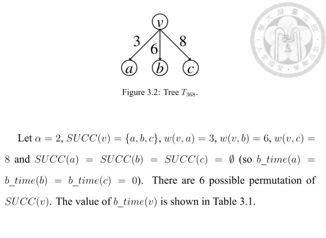
Before introducing this non-sorting method, we explain why the com- parison key isw(v, ui) + b_time(ui) first. We start from a simple exam- ple, the treeT368, which is shown in Figure 3.2.
v
a b c
3 8
6
Figure 3.2: Tree T368.
Letα = 2, SU CC(v) = {a, b, c}, w(v, a) = 3,w(v, b) = 6,w(v, c) = 8 and SU CC(a) = SU CC(b) = SU CC(c) = ∅ (so b_time(a) = b_time(b) = b_time(c) = 0). There are 6 possible permutation of SU CC(v). The value of b_time(v) is shown in Table 3.1.
Table 3.1: Different broadcast sequences may lead to different broadcast time
SU CC(v) b_time(v)
(a, b, c) max({α + 3, 2α + 6, 3α + 8}) = max({5, 10, 14}) = 14 (a, c, b) max({α + 3, 2α + 8, 3α + 6}) = max({5, 12, 12}) = 12 (b, a, c) max({α + 6, 2α + 3, 3α + 8}) = max({8, 7, 14}) = 14 (b, c, a) max({α + 6, 2α + 8, 3α + 3}) = max({8, 12, 9}) = 12 (c, a, b) max({α + 8, 2α + 3, 3α + 6}) = max({10, 7, 12}) = 12 (c, b, a) max({α + 8, 2α + 6, 3α + 3}) = max({10, 10, 9}) = 10
Observe that the minimal value of b_time(v), 10, occurs when the successors ofv are sorted byw(v, ui) + b_time(ui) descendly. The fol- lowing lemma shows that we can obtain the minimum broadcast time if we sort SU CC(v)by w(v, ui) + b_time(ui) descendly.
Lemma 1 Under the constraintSU CC(v) = {s1, s2,· · · , sk},b_time(v) is minimal ifSU CC(v) = (s1, s2,· · · , sk) andw(v, s1) + b_time(s1) ≥ w(v, sj) + b_time(sj)∀i < j.
Proof.
¬(w(v, si) + b_time(si) ≥ w(v, sj) + b_time(sj)∀i < j)
≡ ∃i < j such that w(v, si) + b_time(si) < w(v, sj) + b_time(sj) max(iα + w(v, si) + b_time(si), jα + w(v, sj) + b_time(sj))
= jα + w(v, sj) + b_time(sj)
> jα + w(v, si) + b_time(si) jα + w(v, sj) + b_time(sj)
> iα + w(v, sj) + b_time(sj)
∴ max(iα + w(v, si) + b_time(si), jα + w(v, sj) + b_time(sj)) max(jα + w(v, si) + b_time(si), iα + w(v, sj) + b_time(sj))
⇒ swapping si and sj in SU CC(v) improves b_time(v)
For any initial sequence ofSU CC(v), we can repeat swappingsiand sj until ∄i < j such that w(v, si) + b_time(si) < w(v, sj) + b_time(sj) to improveb_time(v). This meansb_time(v)is minimal ifSU CC(v) = (s1, s2,· · · , sk)andw(v, si)+b_time(si) ≥ w(v, sj)+b_time(sj)∀i < j.
□ After explaining why the comparison key is w(v, ui) + b_time(ui), we introduce the non-sorting method. The algorithm calssifieskvertices (S) to k + 1 lists. The algorithm firstly finds the longest one (u1) and remembers its length. Then, for every vertexui, the algorithm computes the difference between the length ofui and length of u1. The algorithm computes the quotient this difference divided byα(j). Ifj ≤ k, it means the length of ui is short enough and the algorithm puts ui into the last list (listk).
Otherwize, the algorithm puts ui into listj. For each nonempty list, the algorithm moves the element with the shortest length to the end of
the list. Finally, the algorithm concats thesek +1lists by the lsit number.
We will show this non-sorting method does not break the optimalness of the algorithm in the next chapter. The algorithm below describes this non-sorting method.
Algorithm 4 reorder Input:
A vertices set S ={u1, u2,· · · , uk}.
Output:
A permutation of{u1, u2,· · · , uk}.
1: Let u1 be the vertex in S such that
w(v, u1) + b_time(u1) = max({w(v, u) + b_time(u)|u ∈ S}) ;
2: Create k + 1 linked lists, list0, list1,· · · , listk; listj contains vertices ui such that
3: jα ≤ (w(v, u1) + b_time(u1))− (w(v, ui) + b_time(ui)) < (j + 1)α iff 0 ≤ j < k, and
4: kα≤ (w(v, u1) + b_time(u1))− (w(v, ui) + b_time(ui)) iff j = k;
5: Let u∗j be a vertex in listj such that
w(v, u∗j) + b_time(u∗j) = min({w(u, v) + b_time(u)|u ∈ listj}) ;
6: Move u∗j to the end of listj;
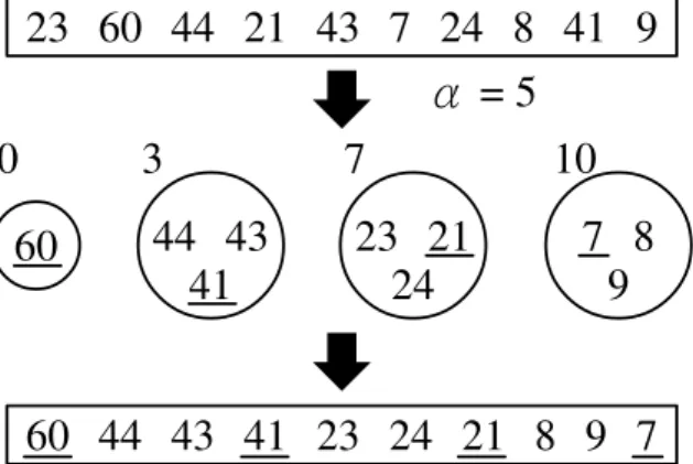
Figure 3.3 shows an example of reordering. In this case,k = 10, the length values are 23, 60, 44, 21, 43, 7, 24, 8, 41, 9 andα = 5.
60 44¡ 43 41
7¡ 8 9 23¡ 21
24
60¡ 44¡ 43¡ 41¡ 23¡ 24¡ 21¡ 8¡ 9¡ 7
0 3 7 10
5
=
23¡ 60¡ 44¡ 21¡ 43¡ 7¡ 24¡ 8¡ 41¡ 9
Figure 3.3: An Example of Reordering.
According to the algorithm, we haveu1 = 60,list0 = {60}withu∗0 = 60,list3 = {44, 43, 41}with u∗3 = 41,list7 = {23, 21, 24} withu∗7 = 21, list10 = {7, 8, 9} with u∗10 = 7 and list1, list2, list4, list5, list6, list8, list9are empty. The reordred sequence is(60, 44, 43, 41, 23, 24, 21, 8, 9, 7).
To make our proof easier, we keep u1 the first place in the buck- eted sequence. Also, we define several terms related to this non-sorting method. A sequence (u1, u2,· · · , uk) is bucketed iff it is a possible output of reorder({u1, u2,· · · , uk}, false). A sequence is deheadedly bucketed iff it is a subsequence(ui, ui+1,· · · , uk)of a bucketed sequence and ui ∈ list/ k. A sequence is reversed bucketed iff it can be obtained from reversing a bucketed sequence.
3.5 Time Complexity
In this section, we discuss the complexity of the algorithm. We analyze the detailed ones before the mainly ones. Complicated analysis is not required.
Lemma 2 Algorithm 4 runs inO(k) time.
Proof. Line 1 takesO(k)time. Line 2 takesO(k)time. The determina- tion from Line 3 to Line 4 takes constant time for eachuiand O(k)time for all vertices inS. Line 5 and Line 6 takes O(|listj|)time forlistj and O(k)time for{list0, list1,· · · , listk}. □
Lemma 3 Algorithm 2 runs inO(k) time.
Proof. Line 1 takes O(k) time. Line 6 to line 10 takes constant time, so Line 5 to line 11 takes O(k) time. Other statements takes constant
time. □
Lemma 4 Algorithm 3 runs inO(k) time.
Proof. Line 3 to line 7 takes constant time, so Line 2 to line 8 takesO(k) time. Other statements takes constant time. □ Theorem 5 Algorithm Broadcast runs inO(n)time.
Proof. Line 2 takes constant time, so the for loop from line 1 to line 3 takesO(n)time. Line 4 takes O(n)time and line 5 takes constant time.
Findingpred(v), SU CC(v), b_time(v)andspare(v)takesO(|N(v)|)time and other statements from line 7 to line 17 takes constant time, so the repeat-until loop from line 6 to line 19 takes
O(∑
v∈V (T )|N(v)|) = O(n)time. □
Chapter 4 Correctness
The goal of this chapter is showing that the proposed algorithm indeed determines the minimal number of centers needed. The optimalness to the algorithm is based on the mutual trust between nodes. That is, every node believes its processed neighbors perform their best, and it can also perform the best to its unprocessed neighbor. The performance of a node v is defined as below:
perf (v, SU CC(v), pred(v)) = (|E−(v)|, b_time(v), spare(v)).
We say(|E−(v)|, b_time(v), spare(v))≤ (|E−′(v)|, b_time′(v), spare′(v)) iff
(1)|E−(v)| < |E−′(v)|, or
(2)|E−(v)| = |E−′(v)|,b_time(v) ≤ b_time′(v) and α + w(u, v) + b_time(v) ≤ t, or
(3)|E−(v)| = |E−′(v)|,α + w(u, v) + b_time(v) > t, α + w(u, v) + b_time′(v) > t,
spare(v) ≤ spare′(v) and spare(v) + α + w(v, u) ≤ t, or
(4)|E−(v)| = |E−′(v)|,α + w(u, v) + b_time(v) > t,
α + w(u, v) + b_time′(v) > t, spare(v) + α + w(v, u) > tand spare′(v) + α + w(v, u) > t. Smaller is better.
The performance of a node is made up of three parts. The first one is unused edges; it depends on the number of successors and whether the node has a predecessor. The second one is its broadcast time; it may affect whether this node can be a successor of its unprocessed neighbor.
The third one is its earliest spare time; it may affect whether this node can be the predecessor of its unprocessed neighbor. In this chapter, we will show the minimalness of|E−(v)|,b_time(v) and spare(v)respectively and then combining them for the correctness of the algorithm.
4.1 Minimum Unused Edges and Broadcast Time
The number of unused edges of v, |E−(v)|, depends on SU CC(v) and pred(v). In this section, we show the algorithm can determine the max- imum of |SUCC(v)| and then discuss the difference between finding pred(v)before and after finding SU CC(v).
Lemma 6 LetSU CC∗(v) ={u1, u2,· · · , uk} and
w(v, u1) + b_time(u1) ≤ w(v, u2) + b_time(u2) ≤ · · · ≤ w(v, uk) + b_time(uk). If we want to choose f nodes from SU CC∗(v) to be the successors, then choosing(uf, uf−1,· · · , u1) isb_time(v)-optimal.
Proof. Suppose we choose (u′f, u′f−1,· · · , u′1). By Lemma 1, we may assume w(v, u′f) + b_time(u′f) ≥ w(v, u′f−1) + b_time(u′f−1) ≥ · · · ≥
w(v, u′1) + b_time(u′1).
Sincew(v, uf) + b_time(uf) ≥ w(v, u′f) + b_time(u′f),
w(v, uf−1) + b_time(uf−1) ≥ w(v, u′f−1) + b_time(u′f−1),· · · , w(v, u1) + b_time(u1) ≥ w(v, u′1) + b_time(u′1),
we haveb_time(v, (uf, uf−1,· · · , u1)) ≥ b_time(v, (u′f, u′f−1,· · · , u′1)).
□ Lemma 7 Using the method in Lemma 6, we can obtain the maximal
number of|SUCC(v)|.
Proof. We can simply choosef such that b_time(v, (uf, uf−1,· · · , u1)) is maximized under the constraintb_time(v, (uf, uf−1,· · · , u1)) ≤ t.□ Lemma 8 Let(u1, u2,· · · , uk)be a bucketed sequence and(u′1, u′2,· · · , u′k) be its sorted permutation; that is, w(v, u′1) + b_time(u′1) ≥ w(v, u′2) + b_time(u′2) ≥ · · · ≥ w(v, u′k) + b_time(u′k).
Then, b_time(v, (u1, u2,· · · , uk)) = b_time(v, (u′1, u′2,· · · , u′k)).
Proof. For each ux ∈ listk, we have arrive(ux) = arrive(v) + xα + w(v, ux)+b_time(ux) ≤ arrive(v)+xα+w(v, u′1)+b_time(u′1)−kα ≤ arrive(v) + w(v, u1) + b_time(u1) = arrive(u1). Let uy = u∗j for some j ∈ {0, 1, · · · , k − 1} and uz ∈ listj − {u∗j}. We have arrive(uy) = arrive(v) + yα + w(v, uy) + b_time(uy) = arrive(v) + yα + w(v, uz) + b_time(uz)−ϵα ≥ arrive(v)+zα+w(v, uz)+b_time(uz) = arrive(uz) for some ϵ such that 0 ≤ ϵ < 1. This means only u∗0, u∗1,· · · , u∗k−1 may dominate b_time(v). Since uy = u′y and the sorted permutation (u′1, u′2,· · · , u′k) is also a bucketed sequence, we have arrive(uy) = arrive(u′y) and therefore this lemma holds. □
Lemma 9 LetSU CC∗(v) ={u1, u2,· · · , uk}. If(u1, u2,· · · , uk) is reversed bucketed sequence, thenb_time(v) = b_time(v, (uf, uf−1,· · · , u1)) wheref is obtained from Lemma 7.
Proof. If listk dominates b_time(v), since we can run Procedure 4 on listk to makelistk bucketed without breaking O(n)-time, by Lemma 8, b_time(v)is optimal. Iflistkdoes not dominateb_time(v), by the same argument in Lemma 8, a vertex in{u∗0, u∗1,· · · , u∗k−1}∩{uf, uf−1,· · · , u1} dominatesb_time(v), so this lemma holds. □ Lemma 10 If we findpred(v)before findingSU CC(v), the performance of v cannot be better.
Proof. If assigning a predecessor causes|SUCC(v)| decreased by two or more,|E−(v)|is increased by at least one. If the|SUCC(v)|does not change, then there are no differences between finding pred(v) before and after findingSU CC(v). If|SUCC(v)|is decreased by one, |E−(v)| does not change; however, it becomes impossible that v ∈ SUCC(u), andspare(v) is increased by at least α due to pred(v)and decreased by at most α thanks to the removed successor of v. □ Lemma 11 Ifv ∈ SUCC∗(u), then v /∈ P RED∗(u).
Proof. If v /∈ SUCC(u), then t− b_time(u) < α, so α + w(v, u) + b_time(u) > t + w(v, u) ≥ t,v cannot be a predecessor candidate of u. Ifv ∈ SUCC(u), since Lemma 10 tells us the performance of v cannot be better ifpred(u) = v, we do not need to include v to P RED∗(u). □
4.2 Earliest Spare Time
We show that the earliest spare time is minimal with a sorting method first, and then we can also obtain the minimum with the non-sorting method. We use notations in Procedure 4.
Lemma 12 ui ∈ listk ⇒ ui can delayα time.
Proof. ui ∈ listk ⇒ w(ui, v)+b_time(ui) ≤ w(u1, v)+b_time(u1)−kα, so(i + 1)α + w(ui, v) + b_time(ui) ≤ (i+1)α+w(u1, v) + b_time(u1)− kα ≤ α + w(u1, v) + b_time(u1) ≤ t. □ Lemma 13 Let ui ∈ listj − {u∗j} for some j ∈ {0, 1, · · · , k − 1}. We haveu∗j can delayα time⇒ ui can delayα time.
Proof. Letu∗j = ui′. We have(i+1)α+w(ui, v)+b_time(ui) ≤ (i′−1+
1)α + w(ui, v) + b_time(ui) < (i′+ 1)α + w(ui′, v) + b_time(ui′) ≤ t.□ Lemma 14 LetSU CC(v) = (u1, u2,· · · , uk). Ifw(v, u1)+b_time(u1) ≥ w(v, u2) + b_time(u2) ≥ · · · ≥ w(v, uk) + b_time(uk), our algorithm can determine the earliest spare timespare(v).
Proof. Ifspare(v) = arrive(v) + (i− 1)α, we need to choose k− isuc- cessors of v, denoted by SU CC′(v), such that b_time(v, SU CC′(v)) ≤ t− arrive(v) − (i − 1)α. By Lemma 6, choosingui+1, ui+2,· · · , uk can obtain minimal b_time(v, SU CC′(v)) under |SUCC′(v)| is fixed by i. Sinceb_time(v, (ui, ui+1,· · · , uk)) ≥ b_time(v, (ui+1, ui+2,· · · , uk)) + α, we havet− arrive(v) − (i − 1)α − b_time(v, (ui+1, ui+2,· · · , uk)) ≤ t− arrive(v) − iα − b_time(v, (ui, ui+1,· · · , uk)). This implies ∃f ∈
{1, 2, · · · , k + 1}such thatb_time(v, SU CC′(v)) ≤ t − arrive(v) − (i − 1)αifi ≥ f andb_time(v, SU CC′(v)) > t−arrive(v)−(i−1)αifi < f and our algorithm determines f and the earliest spare time spare(v) is
exactlyarrive(v) + (f − 1)α. □
Lemma 15 Continued from the previous lemma. If SU CC(v) is de- headedly bucketed, our algorithm can still determine the earliest spare timespare(v).
Proof. Lemma 13 implies the number of successors which can delay α time is equal for any two different deheadedly bucketed sequence of SU CC(v). Since the sorted sequence is also deheadedly bucketed, this number is equal to k − f + 1 where f is introduced in the proof of the
previous lemma. □
4.3 Correctness of the Algorithm
Combining Lemma 7, Lemma 9, Lemma 10 and Lemma 15, we have the result:
Lemma 16 GivenSU CC∗(v)includingb_time(x)∀x ∈ SUCC∗(v)and P ERD∗(v) including spare(p)∀p ∈ P RED∗(v), the algorithm deter- mines SU CC(v) and pred(v) such that perf (v, SU CC(v), pred(v)) is the best.
Before showing the correctness of the algorithm, we still need a lemma:
Lemma 17 LetSU CC∗(v) = {u1, u2,· · · , uk},
SU CC∗(v′) = {u′1, u′2,· · · , u′k},w(v, uj) = w(v′, u′j)∀j ∈ {1, 2, · · · , k}
andarrive(v) = arrive(v′). If∃!i ∈ {1, 2, · · · , k}such thatb_time(u′i) <
b_time(ui) andb_time(uj) = b_time(u′j)∀j ∈ {1, 2, · · · , k} − {i}, then
|SUCC(v′)| ≤ |SUCC(v)| + 1.
Proof. Without loss of generality,
we may assumew(v, ua) + b_time(ua) ≤ w(v, ub) + b_time(ub)∀a < b. Letf = |SUCC(v)|. If |SUCC(v′)| ≥ f + 2, by Lemma 6,
b_time(v′, SU CC(v′)) ≥ b_time(v′,{u′f +2, u′f +1,· · · , u′1}) ≥
b_time(v,{uf +1, uf,· · · , u1}), which means broadcasting cannot be done within the time constraint. Thus,|SUCC(v′)| ≥ f + 2is impossible. □ Theorem 18 Algorithm Broadcast indeed determines the minimal num- ber of centers needed.
Proof. We prove by induction. We want to proof every time a vertex is processed, |E−| = OP T (T − T′, t) − 1; under this condition, for each nodev satisfying v has an unprocessed neighbor,
perf (v, SU CC(v), pred(v)) is minimized.
Letv1 be a leaf of T. Observe that v1 has no choices; that is, SU CC∗(v1) =∅ and P RED∗(v1) =∅
⇒ SUCC(v1) = ∅and pred(v1) = nil
⇒ E−(v1) = 0 = 1− 1 = OP T ({v1}, t) − 1.
∵SU CC(v1) = ∅,∴b_time(v) = 0and spare(v) = 0. Therefore,perf (v1,∅, nil) = (0, 0, 0) is obviously minimal.
Suppose before line 2,|E−| = OP T (T − T′− {v}, t) − 1; under this condition, for each node v satisfying v has an unprocessed neighbor,
perf (v, SU CC(v), pred(v))is minimized. We prove|E−| = OP T (T − T′, t) − 1; under this condition, for each node v satisfying v has an un- processed neighbor,
perf (v, SU CC(v), pred(v)) is minimized.
By Lemma 16, it is impossible to find a strategy to make
perf (v, SU CC(v), pred(v)) smaller without modifying SU CC(x) for some x ∈ T − T′. To make perf (v, SU CC(v), pred(v)) smaller, we have only two choices. The first choice is ∃s ∈ N(v) − {u} such that b_time(s)is decreased, and the other choice is∃p ∈ N(v) − SUCC∗(v) such thatspare(p) is decreased.
For each time the challenger makes a node ∃s ∈ N(v) − {u} such that b_time(s) is decreased, by the induction hypothesis, |E−(s)| must be decreased by at least one. After b_time(s) is decreased, we observe the change ofSU CC(v). Lemma 17 tells usv can accept only one more successor.
If there is a node s′ joining SU CC(v), since b_time(v, SU CC(v)∪ {s′}) ≥ b_time(v, SU CC(v) ∪ {s′} − {s}) ≥ b_time(v, SU CC(v)) and spare(v, SU CC(v) ∪ {s′}) ≥ spare(v, SUCC(v) ∪ {s′} − {s}) ≥ spare(v, SU CC(v)), the challenger fails to make
perf (v, SU CC(v), pred(v)) smaller.
If SU CC(v) is not increased by 1, it is possible v can have a pre- decessor. From pred(v) = nil to pred(v) ̸= nil, spare(v) is increased by at least α. However, making b_time(s) decreased can only make spare(v) decreased by at most α. The challenger still cannot make
perf (v, SU CC(v), pred(v)) smaller.
It is impossible both a nodes′joinsSU CC(v)and frompred(v) = nil to pred(v)̸= nil happen because ∀s∗ ∈ SUCC(v) ∪ {s′},
b_time(v, SU CC(v)∪ {s′} − {s∗}) ≥ b_time(v, SU CC(v)),
sot−arrive(v)−b_time(v, SU CC(v)∪{s′}−{s∗}) ≤ t−arrive(v)−
b_time(v, SU CC(v)), which means v cannot become have ability to have a predecessor after this change by the challenger.
If ∃p ∈ N(v) − SUCC∗(v) such that spare(p) is decreased, by the induction hypothesis,|E−(p)|is decreased by at least one; it can be only made up if pred(v) = nil is changed to pred(v) = p, which makes spare(v)increased by at least α, so perf (v, SU CC(v), pred(v)) cannot
be improved. □
Chapter 5
Two Illustrative Examples
In this chapter, we illustrate the algorithm with two arbitrary trees. Both trees are spanning trees of G0, which is shown in Figure 5.1. Also, we supposeα = 2 and t = 17 in both examples.
3
6 7
4
5 5
2 6 8
2 2
3 3
4
4
5 5 6
4 7
7 8
8
a
v b
c
u
g
x
f w
d e
Figure 5.1: Graph G0.
5.1 The First Example
The tree T1 is shown in Figure 5.2. We demostrate the algorithm twice with two processing sequence,
(a, b, c, d, e, f, g, v, w, x, u)and (g, f, x, e, d, w, u, b, c, v, a). We show the case (a, b, c, d, e, f, g, v, w, x, u)first.