Effects of pad grooves on chemical mechanical planarization

Effects of Pad Grooves on Chemical Mechanical Planarization

Yao-Chen Wang and Tian-Shiang Yang

Department of Mechanical Engineering, National Cheng Kung University, Tainan, Taiwan 70101

Chemical mechanical planarization 共CMP兲 has played an enabling role in producing near-perfect planarity of interconnection and metal layers in ultralarge scale integrated devices. For stable and high performance of CMP, it is important to ensure uniform slurry flow at the pad–wafer interface, hence necessitating the use of grooved pads that help discharge debris and prevent subsequent particle loading effects. Here, using two-dimensional lubrication theory and contact mechanics models, we examine the effects of pad groove designs 共viz. their width, depth, and spacing兲 on slurry flow in CMP. It is found that the presence of pad grooves generally increases the slurry flow rate 共which clearly facilitates debris discharge兲 and the magnitude of the subambient fluid pressure 共i.e., suction兲 on the pad–wafer interface. The increased suction implies higher contact stress on the pad–wafer interface, and hence the local material removal rate is expected to increase as well. However, our numerical results suggest that, as a grooved pad has less contact area for effective interaction with the wafer, the overall material removal rate is expected to increase as well. However, our numerical results suggest that, as a grooved pad has less contact area for effective interaction with the wafer, the overall material removal rate is decreased by the presence of pad grooves. There is therefore a trade-off between slurry flow rate enhancement and material removal rate reduction in pad groove design.

© 2007 The Electrochemical Society. 关DOI: 10.1149/1.2716558兴 All rights reserved.

Manuscript submitted August 15, 2006; revised manuscript received December 1, 2006. Available electronically April 6, 2007.

Chemical mechanical planarization 共CMP兲, also known as chemical mechanical polishing, is now widely recognized as the technology of choice for eliminating topographic variations and achieving near-perfect planarity of interconnection and metal layers in ultralarge scale integrated 共ULSI兲 devices.

During the CMP pro- cess, a rotating wafer is pressed face down against a rotating pad, while a slurry containing chemicals and abrasive particles is dragged into the pad–wafer interface. Polishing is then accomplished by the interaction of the pad and slurry with the wafer surface or by direct contact between the wafer and pad.

To ensure stable and high per- formance of CMP, especially for wafers of larger diameters, it is important to optimize the slurry, pad, and other consumables.

This has thus necessitated the use of grooved pads that help discharge debris and prevent subsequent particle loading effects.

Through theoretical modeling and numerical calculations, this paper aims to understand the effects of pad grooves on slurry flow at the pad–wafer interface, and to gain some insights into the optimi- zation of pad groove designs thereby. In particular, a theoretical model previously used by Shan et al.

is adapted to take into account the presence of grooves on the polishing pad. As a matter of fact, there have been a number of other theoretical models in the literature,

each considering certain aspects of the CMP process.

Specifically, among the works related to the calculation of slurry flow for grooved pads, Subramanian et al.

computed the slurry flow and convective transport of a certain chemical substance in a single two-dimensional groove unit, using finite difference methods and periodic boundary conditions for the fluid pressure and velocity components. 共Similar computations have also been carried out re- cently by Bakhtari et al.

to analyze submicrometer particle re- moval from deep trenches. 兲 While such calculations are capable of capturing certain features of the transport phenomena in a single groove, the fluid dynamic interaction between neighboring grooves 共and that between grooves that are farther apart兲 are inevitably over- looked. Therefore, single-groove calculations generally would not give accurate predictions for the wafer-scale fluid pressure distribu- tion or material removal rate.

For wafer-scale calculations, Muldowney and Tselepidakis

used the commercial software Fluent 6.1 to deal with the compli- cated three-dimensional surface topography of the grooved pad. In their calculations, the grooves were modeled as fluid-filled cells and the asperity layer in the land area of the pad as porous cells 共whose equivalent porosity and characteristic length were determined by an ingenious experimental apparatus; see also Muldowney and James

兲. Of course, the approach of Muldowney and his co-

workers is physically sound and presumably capable of revealing many detailed features of the slurry flow, but the necessity of resolv- ing the slurry flow in each of the numerous grooves on the entire pad generally demands a very large amount of computational re- sources. It then appears to us that, to render the numerical compu- tations less expensive, simpler simulation tools may still be desir- able, and devising such a tool is one of the objectives of this paper.

As noted above, the theoretical model of Shan et al.

was there- fore adapted to take into account the presence of grooves on the polishing pad. Technically, when grooves are present on the pad, the geometry of the interface region apparently varies with time as the wafer slides over the pad surface; calculating the contact stress dis- tribution and slurry flow at the pad–wafer interface is then more difficult than that for flat pads. To reduce the technical difficulties, we have chosen the simplest model that we are aware of 共the model of Shan et al.

兲 to be our point of departure. It is expected, however, that once the technical difficulties arising from the presence of pad grooves are resolved appropriately, similar approaches would also be applicable to other CMP models. Note also that previously Eaton et al.

devised a hybrid Navier–Stokes/lubrication theory approach to calculate the slurry flow for grooved pads. However, while the equivalent thickness of the slurry film is determined from the con- tact stress distribution in the model of Shan et al.

共to be outlined below 兲, it appears that a constant slurry film thickness has to be specified in the approach of Eaton et al.

Therefore, in a certain sense, the present work integrates the groove modeling of Eaton et al.

with the contact stress modeling of Shan et al.

Basically, to simplify matters, Shan et al.

considered a two- dimensional 共2D兲 model problem in which a rigid punch 共modeling the wafer 兲 slides over the surface of an elastic half-space 共modeling the pad 兲 at a constant relative velocity 共see Fig. 1; but disregard the grooves for now 兲. The resulting contact stress on the interface there- fore has a one-dimensional 共1D兲 variation along the direction of the relative sliding velocity, and, for a specified total load on the pad–

wafer interface, can be calculated from an analytical expression of contact mechanics.

Once the contact stress distribution is obtained, the equivalent slurry film thickness 共i.e., the distance between the wafer surface and the mean asperity plane of the pad 兲 is calculated by use of the Greenwood–Williamson contact model for curved surfaces.

Meanwhile, as the 2D slurry flow at the pad–wafer inter- face typically has a small Reynolds number, its dynamics can be described by the Reynolds equation of lubrication theory,

which can also be supplemented with a “flow factor” 共determined from an expression that was deduced by Patir and Cheng

兲 to take into account the reduction of slurry flow rate by surface roughness.

Given the slurry film thickness, the Reynolds equation then can be integrated numerically, yielding the fluid 共slurry兲 pressure distribu- tion on the pad–wafer interface.

z

E-mail: tsyang@mail.ncku.edu.tw

Here we emphasize that, according to the procedure described above, calculating the fluid pressure distribution requires first speci- fying the total load on the pad–wafer interface. However, with a prescribed back pressure on the wafer 共as is usually the case in practice 兲, the total load on the pad–wafer interface 共and hence the contact stress between the wafer and pad 兲 is affected by the fluid pressure distribution on the interface, and therefore is not known a priori. So, it inevitably takes a few iterations to obtain numerical results that observe force balance.

As one can clearly see from the above brief outline, despite being an oversimplification of the realistic CMP process, the model of Shan et al.

still involves rather sophisticated calculations, reflecting the fact that CMP indeed is a complicated process where solid and fluid mechanics 共and slurry chemistry, too兲 may interact in many interesting ways. Nevertheless, Shan et al.

compared their numeri- cal results with experimental data and obtained reasonable agree- ment. One of their major findings was that the average fluid pressure on the pad–wafer interface is typically subambient, and hence in- creases the total load and contact stress on the pad–wafer interface.

Now, as noted above, when grooves are placed periodically on the polishing pad, the geometry of the interface region clearly would change periodically with time as the wafer slides over the pad sur- face at a constant relative speed, resulting in periodic contact stress and fluid pressure variations. From a technical viewpoint, the task we propose to do in this work therefore is more complicated than that of Shan et al.

But once appropriate approaches are devised to resolve the technical difficulties arising from the presence of pad grooves, similar techniques are expected to be applicable to other theoretical models of CMP as well.

In the remainder of this paper, we explain the details of the theoretical model of Shan et al.

and our modifications for incorpo- rating the presence of pad grooves into such a model. Numerical results are then discussed to understand the effects of pad grooves on slurry flow at the pad–wafer interface. Briefly, it turns out that the presence of pad grooves generally increases the slurry flow rate, which clearly facilitates debris discharge. Moreover, compared with a flat pad, the magnitude of the subambient fluid pressure on the pad–wafer interface also is increased by the presence of pad grooves, resulting in higher contact stress on the interface. The local material removal rate therefore is increased according to Preston’s equation.

However, our numerical results suggest that, as a grooved pad has less contact area for the wafer to interact effectively with the polishing pad, the overall material removal rate is de- creased by the presence of pad grooves. There is therefore a trade- off between slurry flow rate enhancement and material removal rate reduction in pad groove design.

Modeling and Numerical Method

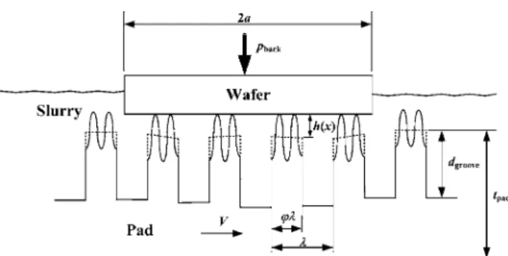
Contact stress distribution on the pad–wafer interface.— Figure 1 shows the schematic of our 2D model problem for CMP. With respect to the 2D rigid punch of width 2a 共hereafter referred to as the “wafer” 兲, the grooved pad slides at a constant speed V. The

coefficient of sliding friction between the pad and wafer surfaces is f, and the Poisson’s ratio of the pad is ␯. Suppose also that the total load on the wafer 共per unit length in the direction normal to the plane shown in Fig. 1 兲 is P, and ignore the presence of pad grooves for now. Then the contact stress distribution on the interface can be calculated from the following expressions

␴

共x兲 = P cos ␲␥

␲共a

− x

兲

冉 ^{a + x a − x} 冊

^关1兴

where

cot ␲␥ = − 2 共1 − ␯兲

f 共1 − 2␯兲 关2兴

and the origin 共x = 0兲 is located at the center of the wafer. Note that Eq. 1 was derived for a 2D rigid punch sliding on the surface of a half space,

and the sliding speed V does not appear explicitly in Eq. 1. Furthermore, denoting the back pressure on the wafer by P

, and the spatial average of fluid pressure on the pad–wafer interface by P

共see Fig. 1兲, we may express the total load P as P = 2a 兵P

− P

其 关3兴 by invoking force balance. Equation 3 clearly indicates that a nega- tive 共i.e., subambient兲 average pressure would increase the total load on the pad–wafer interface. Note also that in practice the wafer typically is pressed against the pad by a fixture with a ball joint, and therefore cannot sustain a moment 共see, for example, Borucki et al.

兲. In other words, the resultant moment with respect to the ball joint due to the contact stress, fluid pressure, and friction acting on the wafer surface has to be zero. This additional requirement amounts to taking into account the wafer surface tilting in the the- oretical model. However, the tilting angle of the wafer surface usu- ally is extremely small 共on the order of a few microradians in the calculations of Jin et al.

兲, so for simplicity we shall not explicitly consider moment balance in the present theoretical model.

Now, when grooves are present, with a fraction ␸ 共0 ⬍ ␸ ⬍ 1兲 of “land area” in each repeating groove unit of length ␭ 共see Fig. 1;

hereafter ␭ is referred to as the “pitch” of the grooves兲, the total load on the pad is carried by the reduced land area, so that the contact stress on the land area is increased by a factor of 1/ ␸. Moreover, the presence of pad grooves renders the geometry of the pad–wafer region varying periodically with time 共with a period of T = ␭/V兲, and hence produces time-periodic contact stress and fluid pressure variations. To incorporate these considerations into our theoretical model, we find it convenient to use the “screening function” ␨共x兲 to mark the position of pad grooves with respect to the wafer at a certain reference instant t = 0; its value is assigned to be unity if the location x corresponds to a point in the land area of the pad and zero otherwise. 关Note that ␨共x兲 is periodic in x with period ␭.兴 Accord- ingly, because the pad is moving at constant speed V with respect to the wafer, the groove position at any instant t is given by

␨共x − Vt兲, which for a fixed location x is time-periodic with period T = ␭/V. Meanwhile, as the geometry of the pad-wafer region changes continuously, the total load on the pad–wafer interface would also vary with time, i.e., P = P 共t兲. Putting together these considerations, we then write the contact stress distribution on the pad–wafer interface as

␴共x,t兲 = ␴

共x,t兲␨共x − Vt兲 = P 共t兲cos ␲␥

␸␲共a

− x

兲

冉 ^{a + x a − x} 冊

^{␨共x − Vt兲}

关4兴 In Eq. 4, ␴

共x,t兲 = ␴

/ ␸ incorporates the time dependence of the total load and the contact stress increase resulting from reduced contact area, while the screening function ␨共x − Vt兲 renders the con- tact stress zero outside the land area 共i.e., over the grooves兲 of the pad. Therefore, one may also think of ␴

共x,t兲 as the contact stress distribution extrapolated outside the land area.

Figure 1. Schematic of the model system 共with compressed asperities and

grooves on the pad 兲.

Note also that in Eq. 4 共and Eq. 1 for flat pads兲 the contact stress

␴共x,t兲 tends to infinity at the two wafer edges x = ± a due to stress concentration. To get around this singularity, following Shan et al.

in numerical calculations we shall exclude a small length ⌬a 共to be specified later 兲 from both edges of the wafer. The computational domain then has a total length of 2 共a − ⌬a兲, and the spatial average of fluid pressure appearing in Eq. 3 can be calculated as

P

共t兲 = 1

2 共a − ⌬a兲 冕

p 共x,t兲dx 关5兴

where p 共x,t兲 is the fluid pressure distribution 共the calculation of which is discussed later 兲. We have checked that the numerical re- sults are not significantly affected by small wafer edge exclusions.

The minor inconsistency of using 2 共a − ⌬a兲 for the total wafer length in Eq. 5 共and other spatial averages兲 therefore are ignored.

Slurry film thickness calculation.— With the contact stress dis- tribution and its temporal variation determined, we then proceed to calculate the equivalent slurry film thickness, which is the distance between the wafer surface and the mean asperity plane of the pad.

To that end, first the extrapolated contact stress distribution ␴

共x,t兲 is used to calculate the corresponding slurry film thickness variation across the wafer. Then, for points over the grooves, the groove depth 共taking into account pad deformation兲 is added to the extrapolated film thickness to yield the total thickness of the slurry film there.

Specifically, assuming Hertzian contact between the pad and wa- fer, the Greenwood–Williamson contact model for curved surfaces relates the extrapolated contact stress distribution to the correspond- ing equivalent slurry film thickness h

共x,t兲 by

␴

共x,t兲 = 4E

3 共1 − ␯

兲 ␩R

冕

⬁

共z − h

兲

␦共z兲dz 关6兴

where E is the elastic modulus of the pad, ␩ and R are the density and average radius of the asperities, respectively, and ␦共z兲 is the distribution function of asperity height. Using an exponential asper- ity height distribution as in Shan et al.,

␦共z兲 = e

/s 共where s is the root-mean-squared average of the pad surface roughness 兲, the inte- gral in Eq. 6 can be readily evaluated, yielding

h

共x,t兲 = s ln

_␲␩ER

s

共1 − ␯

兲␴

共x,t兲 关7兴 Now, to determine the total film thickness over the grooves, we use the Winkler or “mattress” model

and view the land area in each groove unit in Fig. 1 as a column 共a similar approach was also taken in Tichy et al.

兲. When subjected to the compressive contact stress ␴

, the column height will be shortened by an amount of

␴

/K, where the stiffness parameter K is related to the thickness t

and elastic modulus E of the pad. The bottom of a groove, however, is not subjected to significant stress and virtually retains its free 共uncompressed兲 thickness. Therefore, the compressed groove depth under the wafer is calculated to be d

− ␴

/K, where d

is the uncompressed groove depth. Adding then the compressed groove depth to the extrapolated film thickness h

共x,t兲 for points over the grooves, we may write the film thickness distribution across the entire wafer as

h 共x,t兲 = h

共x,t兲 + 关1 − ␨共x − Vt兲兴 · 兵d

− ␴

共x,t兲/K其 关8兴 Note that the factor 1 − ␨共x − Vt兲 on the right side of Eq. 8 vanishes in the land area, and obtains the value of unity over the grooves.

Furthermore, when the contact stress becomes too large so that at certain points ␴

⬎ Kd

关this happens first at wafer edges x = ± 共a − ⌬a兲; see Eq. 4兴, Eq. 8 would give a smaller slurry film thickness for points over a groove than that for points over the land area. This is interpreted as groove failure, and simply indicates that our technical treatment is invalidated when the contact stress is too large. However, in practice the back pressure on the wafer should be

properly set to prevent groove failure, so in our numerical compu- tations the applied pressure and pad parameters are also chosen such that the grooves do not fail.

Reynolds equation for calculating the fluid pressure distribu- tion.— Slurry flow at the pad–wafer interface typically has a small Reynolds number, so that as a good approximation its dynamics is governed by the Reynolds equation of lubrication theory

⳵ h

⳵ t = − ⳵ q

⳵ x = − ⳵

⳵ x 再 ^{Vh 2 − 12 1 ␮ ␺共h兲h}

^{共x,t兲 ⳵ p ⳵ x} 冎 ^关9兴

where p 共x,t兲 is the pressure in the fluid 共slurry兲, ␮ is the viscosity of the fluid. Also, assuming isotropic surface roughness, the volumetric slurry flow rate q 共x,t兲 共per unit wafer breadth兲 is reduced by the

“flow factor” ␺共h兲 = 1.0 − 0.9 exp共−0.56h/s兲, which was deter- mined in a numerical study by Patir and Cheng.

Note that for flat pads, the slurry film thickness would not depend on time,

⳵h/⳵t = 0, and Eq. 9 then reduces to the steady Reynolds equation used in Shan et al.

Numerical method.— To obtain the temporal variation of the fluid pressure distribution, one has to integrate Eq. 9 numerically, and here we discuss the technicalities. First, we discretize the ⳵h/⳵t term of Eq. 9 in a two-step implicit manner, yielding

1

⌬t 兵h

共x兲 − h

共x兲其 = − ⳵

⳵ x 再 ^{V 2 h}

^{共x兲 − 12 1 ␮ ␺共h}

^兲

⫻关h

共x兲兴

⳵

⳵ x 关p

共x兲兴 冎 ^关10兴

where ⌬t is the discrete time step 共to be specified later兲, h

共x兲

= h 共x,共n + 1兲⌬t兲 and p

共x兲 = p关x,共n + 1兲⌬t兴 are the slurry film thickness and pressure distributions at the discrete time instant t = 共n + 1兲⌬t. Note that Eq. 10 is implicit in the sense that its right side involves slurry film thickness and pressure distributions that are unknown as yet. Furthermore, the spatial partial derivatives on the right side of Eq. 10 are discretized using standard central-difference schemes

共the results are not elaborated here for brevity兲. For given slurry film thickness distributions h

共x兲 and h

共x兲, together with the boundary condition that the fluid pressure is equal to the atmo- spheric pressure at the wafer edges x = ± 共a − ⌬a兲, we have a well-posed matrix inversion problem for calculating the fluid pres- sure distribution p

共x兲.

However, calculation of h

共x兲 requires first calculating the extrapolated contact stress distributions ␴

关x,共n + 1兲⌬t兴, which, in turn, depends on the total load P

= P 关共n + 1兲⌬t兴 at the corre- sponding instant 共see Eq. 4, 7, and 8兲. But as pointed out earlier, the total load P

depends on both the applied back pressure on the wafer 共which can be prescribed兲 and the average fluid pressure 共which remains to be calculated, however兲; a few iterations therefore are needed to obtain a converged solution of the fluid pressure dis- tribution p

共x兲. Specifically, at each discrete time instant t = 共n + 1兲⌬t, an initial guess of the total load P

is made to start the iterations. After going through the procedures described above to obtain the fluid pressure p

共x兲, we can use Eq. 5 to calculate its spatial average, and use Eq. 3 to calculate the corresponding total load. The initial guess is then compared with the total load P

just calculated, and corrected by Newton’s method.

After a few iterations, a converged solution generally is obtained, and one can move on to the next discrete time instant.

But there is one final loose end to tie up for the calcu-

lation procedures. Specifically, at the very beginning of the

calculations 共corresponding to n = 0兲, the slurry film thickness

h

共x兲 = h

共x兲 = h共x,0兲, which also is essential for starting the

calculations, is not known, because it depends on the total load

P

= P

= P 共0兲 that cannot be specified arbitrarily. 共The groove

position relative to the wafer can be specified arbitrarily for t = 0,

but the corresponding fluid pressure distribution needs to be calcu- lated. 兲 To resolve this difficulty, recall that the geometry of the pad–

wafer region varies periodically with period T. The total load P 共t兲 therefore should also be a periodic function of the same period, and it suffices to calculate the slurry flow for a complete period only. A tentative value of P

= P 共0兲 therefore is specified, so that the ini- tial slurry film thickness h

共x兲 can be obtained from Eq. 4, 7, and 8 to start the calculations. After calculating for a complete period, the resulting total load P 共T兲 is compared with the tentative initial value P 共0兲; if the difference exceeds a preset tolerance, we then update P 共0兲 by P共T兲 and carry out the calculations for one more period. Whether this iteration scheme does yield a solution for P 共0兲, and how to choose a solution when there are many, are discussed below for specific parameter values.

Results and Discussion

In all computations, the pad properties 共listed in Table I兲 are taken to be the same as those used in Shan et al.,

and the viscosity of water at room temperature ␮ = 0.001 Pa · s is used for the slurry.

The half-width of the wafer is taken to be a = 50 mm, the wafer- edge exclusion distance ⌬a = 5 mm, the applied back pressure on the wafer p

= 20 kPa, and the relative sliding speed V

= 0.43 m/s, as in Shan et al.

Furthermore, following Tichy et al.,

the stiffness parameter for calculating the compressed groove depth is taken to be K = 2.5 MPa/mm 共corresponding to a pad thickness on the order of a few millimeters 兲. The friction coefficient between the pad and wafer surfaces is f = 0.8. The effects of the land-area fraction ␸, number of grooves under the wafer N 关related to the pitch of the grooves by ␭ = 2共a − ⌬a兲/N兴, and uncompressed groove depth d

on slurry flow are investigated; their values are speci- fied in the ensuing discussion.

As for the grid size and discrete time step used in the computa- tions, we divide the computational domain into 18,000 equal divi- sions 关the grid size therefore is ⌬x = 2共a − ⌬a兲/18,000 = 5 ␮m兴 so that even the narrowest grooves encountered in the computations can be adequately resolved. Moreover, the discrete time step is cho- sen to be ⌬t = ⌬x/V, so that in each time step the pad moves a distance of ⌬x exactly. It has also been checked that reducing the grid size 共and the corresponding time step兲 does not alter the nu- merical results significantly.

Solution existence and stability issues.— First, let us check if our iteration scheme does produce solutions that make physical sense. As an example, suppose that there are 30 grooves under the wafer 共N = 30兲, so that the pitch of the grooves ␭ = 3 mm and the period of the slurry flow T = ␭/V = 6.98 ms. It was pointed out above that a tentative value of P

= P 共0兲 共or, equivalently, a value of the spatially averaged fluid pressure p

共0兲 for prescribed back pressure on the wafer; see Eq. 3 兲 has to be specified to start the calculations, and an admissible periodic solution of slurry flow re- quires that the resulting total load P 共T兲 = P共0兲 关or p

共T兲

= p

共0兲兴. To see how p

共T兲 varies with p

共0兲, for a range of input values of p

共0兲 we carry out the computations for one com- plete period, and plot the resulting values of the fluid pressure mis- match p

共0兲 − p

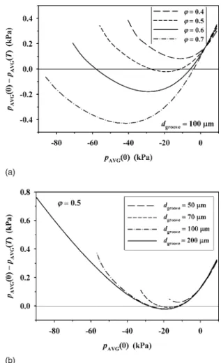
共T兲 in Fig. 2. In particular, in Fig. 2a, the fluid pressure mismatch is plotted as a function of the input pressure

p

共0兲 for various values of the land-area fraction ␸, taking the uncompressed groove depth d

= 100 ␮m, while in Fig. 2b the fluid pressure mismatch is plotted for various d

, taking

␸ = 0.5. Note also that the range for the input pressure p

共0兲 is chosen such that no groove failure 共which invalidates our theoretical model 兲 occurs. For example, for d

= 100 ␮m and ␸ = 0.5 共see Fig. 2a 兲, groove failure is encountered if p

共0兲 ⬍ −56 kPa; so the computations are not carried out beyond that pressure.

Now, the results in Fig. 2a indicate that, for a prescribed uncom- pressed groove depth, no periodic solutions exist if the land-area fraction is too small 关␸ ⬍ 0.483 for d

= 100 ␮m兴. Meanwhile, Fig. 2b shows that, for a given land-area fraction, the groove depth has to be large enough 共d

⬎ 61 ␮m for ␸ = 0.5兲 for periodic solutions to exist. Recall that a smaller value of ␸ implies less con- tact area and hence larger contact stress. Moreover, increased con- tact stress results in greater pad deformation that might cause groove failure for smaller groove depths. We therefore conjecture that the nonexistence of solutions when ␸ or d

is too small implies that in such cases the pad is not strong enough to support the wafer 共in relative sliding motion 兲 without groove failure.

It is also seen in Fig. 2a that for a range of ␸ values 共e.g., ␸

= 0.5 or 0.6 兲, there may exist two periodic solutions for the slurry flow. Note, however, that at the two solutions the curve of pressure mismatch has slopes of opposite signs, so that the two solutions have different stability properties. Specifically, for the solution hav- Table I. Pad properties (corresponding to Rodel ICI000 pad;

adapted from Shan et al.

).

Parameters Values

Elastic modulus E = 12.01 Mpa

Surface roughness Ra = 5 ␮m, rms s = 6 ␮m

Poisson’s ratio ␯ = 03

Asperity density ␩ = 400 mm

Average radius of asperities R = 0.1 mm

Figure 2. Computed spatial average of the fluid pressure at t = T, p

共T兲;

for a range of prescribed values of p

共0兲. Here N = 30 and plotted are 共a兲 the fluid pressure mismatch p

共0兲 − p

共T兲 as a function of p

共0兲 for various values of the land-area fraction ␸, taking the uncompressed groove depth d

= 100 ␮m. 共b兲 Pressure mismatch for various d

, taking

␸ = 0.5. Other parameter values are detailed in the text.

ing a smaller magnitude of 兩p

共0兲兩, the slope of the pressure mismatch curve is positive. This means that if the input pressure p

共0兲 is slightly perturbed for some reason, the resulting aver- aged pressure p

共T兲 will tend to be restored to the correct value of p

共0兲 after one period. That solution is therefore stable from a physical point of view, while the other solution can be shown to be unstable by a similar argument. Moreover, from the standpoint of numerical computations, when there indeed exists a stable solution, our iteration scheme will always converge to that solution with a reasonable initial guess of p

共0兲. Therefore, it is both physically and numerically sound that the ensuing discussion only concerns stable solutions for the slurry flow.

An additional observation in Fig. 2a is that, as the land-area fraction keeps on increasing 共for fixed groove depth兲, the magnitude 兩p

共0兲兩 of both the stable and unstable solutions increase; the unstable solution may eventually cause groove failure and then

“cease” to exist in Fig. 2a 共as the computations were not carried out beyond groove failure 兲. Finally, as shown in Fig. 2b, for a given land-area fraction, both the stable and unstable solutions of p

共0兲 become relatively independent of groove depth when the groove depth exceeds a certain value 共roughly when d

⬎ 100 ␮m for

␸ = 0.5兲.

Basic features of the slurry flow dynamics.— Having addressed the issues of solution existence and selection, here we proceed to describe the basic features of slurry flow dynamics. As a particular example, let us take N = 30 as before 共so that ␭ = 3 mm and T = ␭/V = 6.98 ms兲, and, in addition, ␸ = 0.9 and d

= 200 ␮m; the groove width therefore is ␭共1 − ␸兲 = 0.3 mm. The above parameter values are typical for commercial pads.

Using the parameter values specified above, the temporal varia- tion of the spatial average of fluid pressure p

共t兲 is calculated, and the result is shown in Fig. 3. As was observed by Shan et al.,

here the average pressure is negative, and hence produces a suction force that increases the contact stress on the pad–groove interface.

Also, because the slurry flow is periodic with time, the reference instant t = 0 does not have an absolute meaning. It is simply as- signed here to the very instant when a groove is about to go under the wafer at x = −a 共recall, however, that the computational domain extends from x = −a + ⌬a to a − ⌬a兲, as can be seen in Fig. 4 where the equivalent slurry film thickness distributions at t = 0 and T/2 are shown. Note that in Fig. 4 the “spikes” of larger film thick- nesses correspond to the groove locations. Also, the right and left halves of Fig. 4 are plotted using different scales for x, so that both the wafer-wide and local film thickness variations can be clearly shown. 共The envelope of the wafer-wide film thickness distribution is approximately symmetric with respect to the origin x = 0. 兲

Moreover, Fig. 3 indicates that the relatively small groove size here 共compared with the wafer half-length a兲 only produces an av- erage fluid pressure variation on the order of a few Pa’s 共while the back pressure on the wafer is 20 kPa 兲. As a result, the spatial distri- bution of fluid pressure p 共x,t兲 would only have a relatively weak dependence on time, as is illustrated in Fig. 5. However, Eq. 9 indicates that the volumetric slurry flow rate q 共x,t兲 has a cubic de- Figure 3. Variation of the spatial average of fluid pressure with time, for

N = 30, ␸ = 0.9, and d

= 200 ␮m 共other parameter values are detailed

in the text 兲. Here the period of slurry flow is T = 6.98 ms. Figure 4. Slurry film thickness distributions at t = 0 and T/2, for N = 30,

␸ = 0.9, and d

= 200 ␮m.

Figure 5. Fluid pressure distributions at t = 0 and T/2, for N = 30,

␸ = 0.9, and d

= 200 ␮m. 共a兲 Wafer-wide pressure distribution. 共b兲

Close-up of the first few groove cycles.

pendence on h 共x,t兲 and hence is much more sensitive to the film thickness variation than the fluid pressure, resulting in the significant flow rate variations shown in Fig. 6 for t = 0 and T/2. 共Like Fig. 4, the right and left halves of Fig. 6 are plotted using different scales for x; the envelope of the wafer-wide slurry flow rate distribution is approximately symmetric with respect to the origin x = 0. 兲 Looking more closely at the first few groove cycles 共Fig. 5b兲, one also ob- serves that the pressure gradient 兩⳵p/⳵x兩 in a groove is smaller than that in the land area, because the slurry film thickness is larger 共corresponding to a smaller flow resistance兲 in a groove.

We now have a pretty good understanding about the basic slurry flow dynamics, and may go on to examine the effects of various pad groove parameters such as the land-area fraction ␸, number of grooves under the wafer N, and uncompressed groove depth d

on the slurry flow dynamics. In particular, we wish to see how and to what extent the average fluid pressure and slurry flow rate vary with the aforementioned groove parameters. Moreover, the simple model of the Preston’s equation

are used to calculate the depen- dence of the material removal rate on the groove pattern design characterized by such parameters.

Dependence of the averaged fluid pressure on pad groove pa- rameters.— Recall that the spatial average of fluid pressure p

共t兲 is a measure of the resultant force acting on the wafer by the slurry 共see Eq. 5兲. The contact stress on the pad–wafer interface 共and the material removal rate 兲 therefore would be dependent upon the aver- aged fluid pressure. As shown in Fig. 3, however, the spatially av- eraged fluid pressure varies periodically with time. Therefore, to examine the dependence of the spatially averaged fluid pressure on various groove parameters, we find it useful to calculate the tempo- ral mean of p

共t兲

具p

典 = 1 T 冕

T

p

共t兲dt 关11兴

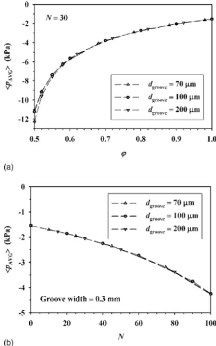
In Fig. 7, the calculated mean values of the spatially averaged fluid pressure are plotted for a number of uncompressed groove depths: d

= 70, 100, and 200 ␮m. In particular, in Fig. 7a, the groove number is kept constant 共N = 30兲, while the land-area ratio

␸ is being varied. Note that in such cases, larger values of ␸ corre- spond to narrower grooves, and the limiting case ␸ = 1 corresponds to a flat pad 共without any grooves兲. Meanwhile, in Fig. 7b the groove width is fixed to be 0.3 mm. Increasing the groove number then corresponds to reducing the pitch of the grooves and reducing the land-area ratio ␸ accordingly, with the limiting case N → 0 again corresponding to a flat pad. It is seen in both Fig. 7a and b that the mean value of the spatially averaged fluid pressure 具p

典 gen- erally is negative, consistent with the experimental and numerical

results for flat pads in Shan et al.

Furthermore, the magnitude of 具p

典 increases as the land-area ratio ␸ decreases 共and, equiva- lently, as the number of grooves N increases 兲. This in fact can be understood on physical grounds: as ␸ decreases, the pad has to sustain higher contact stress, resulting in a smaller slurry film thick- ness and hence a larger flow resistance, so that the averaged fluid pressure is higher. An additional observation in Fig. 7 is the rather weak dependence of 具p

典 on the groove depth. Like the results shown in Fig. 3, this again points to the fact that the relatively small size of the grooves does not affect the fluid pressure significantly.

Dependence of the mean slurry flow rate on pad groove param- eters.— Here we calculate the mean value of the volumetric slurry flow rate

具q典 = 1 T 冕

T

q 共x,t兲dt 关12兴

and discuss its dependence on various groove parameters. Note that, as can be readily deduced from Eq. 9 共which is a statement of mass conservation in essence 兲, the mean value of the slurry flow rate 具q典 does not depend on the spatial variable x. It is expected that a larger flow rate would facilitate discharge debris, and hence is beneficial for the CMP process.

Now, for the same groove parameter combinations used to obtain the results shown in Fig. 7, the calculated mean slurry flow rates are plotted in Fig. 8. Despite that the mean value of the spatially aver- aged fluid pressure appears to be relatively independent of the groove depth in Fig. 7, here in Fig. 8 the mean flow rate increases Figure 6. Spatial variations of the volumetric slurry flow rate 共per unit wafer

breadth 兲 at t = 0 and T/2, for N = 30, ␸ = 0.9, and d

= 200 ␮m. Here the time-averaged flow rate 具q典 = 0.1373 cm

/s.

Figure 7. Mean values of the spatially averaged fluid pressure 具p

典 for

various uncompressed groove depths. 共a兲 Dependence of 具p

典 on the land-

area ratio ␸ for N = 30. 共b兲 Dependence of 具p

典 on the groove number N

for groove width ␭共1 − ␸兲 = 0.3 mm.

dramatically with the groove depth. As pointed out earlier, this re- sults from the fact that the volumetric slurry flow rate has a cubic dependence on the slurry film thickness 共see Eq. 9兲. More impor- tantly, both Fig. 8a and b indicate that the slurry flow rate generally increases with decreasing land-area ratio 共and, equivalently, with increasing groove number N 兲. In other words, increasing the number and/or width of the grooves generally increases the slurry flow rate.

Note, however, that as seen in Fig. 8a, for smaller groove depths, the mean slurry flow rate may reach a local maximum at a particular small land-area fraction 共e.g., ␸ ⬇ 0.52 for d

= 70 ␮m兲. This is related to the fact that the pad deformation increases as the land- area fraction decreases, resulting in smaller compressed groove depths that prevent further slurry flow rate increase.

From the results shown in Fig. 7 and 8, it can be concluded that, from the viewpoint of debris discharge, placing grooves on the pad is beneficial for the CMP process. Meanwhile, as the presence of pad grooves generally increases the contact stress on the pad–groove interface, the local material removal rate is expected to increase as well. However, placing grooves on the pad also reduces the land area of the pad for effective interaction with the wafer, and hence tends to decrease the overall material removal rate. It is therefore not clear at this moment whether the overall material removal rate is increased or decreased. This issue is addressed below using the simple model of the Preston’s equation.

Dependence of the overall material removal rate on pad groove parameters.— Here we assume that the local material removal rate R ˙ 共x,t兲 is related to the contact pressure p

− p 共x,t兲 and sliding speed V between the wafer and pad by the Preston’s equation

R ˙ 共x,t兲 = C

兵p

− p 共x,t兲其V 关13兴 where C

is usually referred to as Preston’s constant. To have a reasonable estimate for the value of C

, we have compared the ex- perimental data of Thagella et al.,

for silicon oxide with numerical results obtained by using our theoretical model. 共Note that their data of material removal rate appear to be for flat pads. The geometry of the pad–wafer region therefore does not change with time; so it suffices to use the steady version of Eq. 9 and the numerical calcu- lation is greatly simplified. 兲 As shown in Fig. 9, the data of Thagella et al.

can be fitted with reasonable accuracy 共minimized root- mean-squared error 兲 by C

= 4.35 ⫻ 10

Pa

for p

= 3 psi 共20.68 kPa兲, 0.2 ⬍ V ⬍ 1.2 m/s; and by C

= 3.67 ⫻ 10

Pa

for V = 0.8 m/s, 10 ⬍ p

⬍ 40 kPa. Here, the back pressure and sliding speed ranges cover the particular combination of p

= 20 kPa and V = 0.43 m/s that has been used in our calculations.

Note also that the estimated values of the Preston’s constant for the two cases are close to each other; so we shall simply take their arithmetic mean C

= 4.0 ⫻ 10

Pa

in subsequent calculations of material removal rate for grooved pads.

For grooved pads, however, we shall make an additional assump- tion that only the land area of the pad in contact with the wafer polishes effectively, while polishing by the groove area practically is negligible. To calculate the overall material removal rate, therefore, one has to take into account the instantaneous groove position, and the spatial average of the removal rate is calculated to be

R ˙

AVG

共t兲 = 1

2 共a − ⌬a兲 冕

R ˙ 共x,t兲␨共x − Vt兲dx 关14兴 Recall that ␨共x − Vt兲 is the screening function defined earlier to represent the instantaneous position of the grooves with respect to Figure 8. Mean values of the volumetric slurry flow rate 具q典 for various

uncompressed groove depths. 共a兲 Dependence of 具q典 on the land-area ratio ␸ for N = 30. 共b兲 Dependence of 具q典 on the groove number N for groove width

␭共1 − ␸兲 = 0.3 mm.

Figure 9. Comparison of experimental data of material removal rates

共adapted from Thagella et al.

兲 with the predictions of Preston’s equation.

the wafer; its value is unity in the land area and zero otherwise.

Furthermore, after one complete groove cycle, the mean value of the material removal rate is calculated to be

MRR = 1 T 冕

T

R ˙

AVG

共t兲dt 关15兴

Now, the calculated mean material removal rates are plotted in Fig. 10, again for the same groove parameter combinations used to obtain the results shown in Fig. 7. First, it is readily seen in Fig. 10 that, just like the pressure distributions, the material removal rate only has a relatively weak dependence on the groove depth. Further- more, as it turns out, the overall material removal rate decreases with decreasing land-area ratio ␸ for N = 30, and decreases with increasing N for the fixed groove width of 0.3 mm. In other words, despite that the presence of pad grooves increases the contact stress on the pad–groove interface, and hence the local material removal rate, the land area of the pad is reduced to a greater extent so that the overall material removal rate is decreased. Note also that the MRR curves in Fig. 10a appear to reach a local minimum at ␸ ⬇ 0.54.

Like the local maximum of slurry flow rate observed in Fig. 8a, this is related to the reduced slurry film thickness for smaller values of

␸. The resulting higher flow resistance then increases the average fluid pressure, and hence prevent the material removal rate from further decrease. However, as the land-area fraction ␸ keeps on decreasing, the grooves soon would fail, before much increase of the material removal rate could result.

The major advantage of placing grooves on the pad therefore seems to be the resulting greater slurry flow rate for debris dis- charge, at the expense of reducing the overall material removal rate.

So, for practical groove pattern design, a careful decision must be made to achieve an optimized trade-off between the material re- moval rate reduction and sufficient slurry flow rate for debris dis- charge. Furthermore, although the average fluid pressure and overall material removal rate are relatively independent of the uncom- pressed groove depth, increasing the groove depth generally would increase the slurry flow rate significantly and reduce the possibility of groove failure. It is therefore advisable to use deeper grooves, as long as the land area of the pad does not buckle under the applied load.

Conclusion

Here, using two-dimensional lubrication theory supplemented with contact mechanics models, we have examined the effects of various pad groove parameters, such as the groove width, depth, and spacing, on the slurry flow dynamics and material removal rate. As oversimplified as our theoretical model may seem, we expect that the approach devised in this study to resolve the technical difficul- ties arising from the presence of pad grooves would also be appli- cable to other CMP models.

As it turns out, for uncompressed groove depths greater than about 100 ␮m, the fluid pressure and contact stress on the pad–

wafer interface are essentially independent on the groove depth.

However, the presence of pad grooves generally increases the slurry flow rate significantly, and therefore is beneficial for debris dis- charge. It is also found that the magnitude of the subambient fluid pressure on the pad–wafer interface is increased by the presence of pad grooves. As the increased suction pressure implies higher con- tact stress between the pad and wafer, the local material removal rate therefore is increased as well. Nevertheless, our numerical results suggest that, because a grooved pad has less contact area with the wafer for effective polishing, the overall material removal rate is decreased by the presence of pad grooves. It is therefore concluded that the major advantage of placing grooves on the pad is the result- ing greater slurry flow rate for debris discharge, while the overall material removal rate is reduced to some extent. Therefore, for groove pattern design in practice, one must seek an optimized trade- off between the material removal rate reduction and slurry flow rate increase. Moreover, as long as the land area of the pad does not buckle, it is advisable to use deeper grooves, as they would signifi- cantly increase the slurry flow rate and reduce the possibility of groove failure, without much sacrifice of the overall material re- moval rate.

Acknowledgments

The authors gratefully acknowledge generous support of this work by the Taiwan Semiconductor Manufacturing Company 共TSMC兲 through grants NCKU-0403 and NCKU-0603. They also thank Dr. S.-M. Cheng, Dr. T.-C. Tseng, Dr. Y.-W. Chou, and Dr.

J.-C. Sheu of TSMC, and Professor K.-S. Chen of NCKU, for a number of fruitful discussions on this work and other related topics.

Moreover, the authors thank two anonymous reviewers for bringing a number of related works to their attention, thereby helping to improve this paper. The work of T.S.Y. has also been supported by the R.O.C. 共Taiwan兲 National Science Council, recently through grant NSC95-2221-E-006-045-MY2.

National Cheng Kung University assisted in meeting the publication costs of this article.

References

1. R. K. Singh and R. Bajaj, MRS Bull., 27, 743 共2002兲.

2. W. J. Patrick, W. L. Guthrie, C. L. Standley, and P. M. Schiable, J. Electrochem.

Soc., 138, 1778

共1991兲.

3. R. K. Singh, S.-M. Lee, K.-S. Choi, G. B. Basim, W. Choi, Z. Chen, and B. M.

Moudgil, MRS Bull., 27, 752 共2002兲.

4. M. Moinpour, A. Tregub, A. Oehler, and K. Cadien, MRS Bull., 27, 766 共2002兲.

5. T. K. Doy, K. Seshimo, K. Suzuki, A. Philipossian, and M. Kinoshita, J. Electro- Figure 10. Mean values of the overall material removal rate MRR for vari-

ous uncompressed groove depths. 共a兲 Dependence of MRR on the land-area

ratio ␸ for N = 30. 共b兲 Dependence of MRR on the groove number N for

groove width ␭共1 − ␸兲 = 0.3 mm.

chem. Soc., 151, G196

共2004兲.

6. D. Rosales-Yeomans, T. Doi, M. Kinoshita, T. Suzuki, and A. Philipossian, J.

Electrochem. Soc., 152, G62

共2005兲.

7. L. Shan, J. Levert, L. Meade, J. Tichy, and S. Danyluk, Trans. ASME, J. Tribol.,

共2000兲.

8. S. Sundararajan, D. G. Thakurta, D. W. Schwendeman, S. P. Murarka, and W. N.

Gill, J. Electrochem. Soc., 146, 761 共1999兲.

9. J. Tichy, J. A. Levert, L. Shan, and S. Danyluk, J. Electrochem. Soc., 146, 1523 共1999兲.

10. D. G Thakurta, C. L. Borst, D. W. Schwendeman, R. J. Gutmann, and W. N. Gill,

共2000兲.

11. S. R. Harp and R. F. Salant, ASME J. Lubr. Technol., 123, 134 共2001兲.

12. A. T. Kim, J. Seok, J. A. Tichy, and T. S. Cale, J. Electrochem. Soc., 150, G570 共2003兲.

13. X. Jin, L. M. Keer, and Q. Wang, J. Electrochem. Soc., 152, G7 共2005兲.

14. C. F. Higgs III, S. H. Ng, L. Borucki, I. Yoon, and S. Danyluk, J. Electrochem.

Soc., 152, G193

共2005兲.

15. R. S. Subramanian, L. Zhang, and S. V. Babu, J. Electrochem. Soc., 146, 4263 共1999兲.

16. K. Bakhtari, R. O. Guldiken, A. A. Busnaina, and J.-G. Park, J. Electrochem. Soc.,

153, C603

共2006兲.

17. G. P. Muldowney and D. P. Tselepidakis, in Proceedings of the 2004 CMP-M1C

共2004兲.

18. G. P. Muldowney and D. B. James, Mater. Res. Soc. Symp. Proc., 816, 147 共2004兲.

19. J. K. Eaton, C. J. Elkins, T. M. Burton, A. Miyaji, and D. P. Coon, in Proceedings

共2003兲.

20. K. L. Johnson, Contact Mechanics, p. 41 and 104, Cambridge University Press, Cambridge, UK 共1985兲.

21. J. A. Greenwood and J. B. P. Williamson, Proc. R. Soc. London, Ser. A, 295, 300 共1966兲.

22. B. J. Hamrock, S. R. Schmid, and B. O. Jacobson, Fundamentals of Fluid Film

共2004兲.

23. N. Patir and H. S. Cheng, ASME J. Lubr. Technol., 100, 12 共1978兲.

24. F. Preston, J. Soc. Glass Technol., 11, 214 共1927兲.

25. L. J. Borucki, S. H. Ng, and S. Danyluk, J. Electrochem. Soc., 152, G391 共2005兲.

26. J. C. Tannehill, D. A. Anderson, and R. H. Pletcher, Computational Fluid Mechan-

共1997兲.

27. C. Gerald and P. O. Wheatley, Applied Numerical Analysis, 6th ed., p.48, Addison- Wesley, Reading, MA 共1999兲.

28. S. Thagella, A. K. Sikder, and A. Kumar, J. Electrochem. Soc., 151, G205 共2004兲.