1-1
Introduction To Modeling
Chapter 1
Copyright © 2010 Pearson Education, Inc. Publishing as Prentice Hall Copyright © 2010 Pearson Education, Inc. Publishing as Prentice Hall 1-2
Chapter Topics
The Management Science Approach to Problem Solving
Model Building: Break-Even Analysis
Computer Solution
Management Science Modeling Techniques
Business Usage of Management Science Techniques
Management Science Models in Decision Support Systems
The Management Science Approach
Management science uses a scientific approach to solving management problems.
It is used in a variety of organizations to solve many different types of problems.
It encompasses a logical mathematical approach to problem solving.
Management science, also known as operations research, quantitative methods, etc., involves a philosophy of problem solving in a logical manner.
Figure 1.1
The Management Science Process
1-5 Copyright © 2010 Pearson Education, Inc. Publishing as Prentice Hall
Observation - Identification of a problem that exists (or may occur soon) in a system or organization.
Definition of the Problem - problem must be clearly and consistently defined, showing its boundaries and interactions with the objectives of the organization.
Model Construction - Development of the functional mathematical relationships that describe the decision variables, objective function and constraints of the problem.
Model Solution - Models solved using management science techniques.
Model Implementation - Actual use of the model or its solution.
1-6 Copyright © 2010 Pearson Education, Inc. Publishing as Prentice Hall
Information and Data:
Business firm makes and sells a steel product
Product costs $5 to produce
Product sells for $20
Product requires 4 pounds of steel to make
Firm has 100 pounds of steel Business Problem:
Determine the number of units to produce to make the most profit, given the limited amount of steel available.
Example of Model Construction (1 of 3)
Variables: X = # units to produce (decision variable) Z = total profit (in $)
Model: Z = $20X - $5X (objective function) 4X = 100 lb of steel (resource constraint) Parameters: $20, $5, 4 lbs, 100 lbs (known values) Formal Specification of Model:
maximize Z = $20X - $5X subject to 4X = 100
Example of Model Construction (2 of 3) Example of Model Construction (3 of 3)
Solve the constraint equation:
4x = 100
(4x)/4 = (100)/4 x = 25 units
Substitute this value into the profit function:
Z = $20x - $5x
= (20)(25) – (5)(25) = $375
(Produce 25 units, to yield a profit of $375)
Model Solution:
1-9 Copyright © 2010 Pearson Education, Inc. Publishing as Prentice Hall
Model Building:
Break-Even Analysis (1 of 12)
■ Used to determine the number of units of a product to sell or produce that will equate total revenue with total cost.
■ The volume at which total revenue equals total cost is called the break-even point.
■ Profit at break-even point is zero.
1-10 Copyright © 2010 Pearson Education, Inc. Publishing as Prentice Hall
Model Components
Volume (v) – the number of units produced or sold
Fixed Cost (c
f) - costs that remain constant regardless of number of units produced.
Variable Cost (c
v) - unit production cost of product.
Total variable cost (vc
v) - function of volume (v) and unit variable cost.
Model Building:
Break-Even Analysis (2 of 12)
Model Components
Total Cost (TC) - total fixed cost plus total variable cost.
Profit (Z) - difference between total revenue vp (p = unit price) and total cost, i.e.
Model Building:
Break-Even Analysis (3 of 12)
v
f
vc
c TC = −
v f
- vc vp - c Z =
Model Building:
Break-Even Analysis (4 of 12)
Computing the Break-Even Point
The break-even point is that volume at which total revenue equals total cost and profit is zero:
v f
f v
v f
c p v c
c c p v
vc c vp
= −
=
−
=
−
− ) (
0
The break-even point
1-13 Copyright © 2010 Pearson Education, Inc. Publishing as Prentice Hall
Break-Even Analysis (5 of 12)
Example: Western Clothing Company
Fixed Costs: c
f= $10,000 Variable Costs: c
v= $8 per pair Price : p = $23 per pair
The Break-Even Point is:
v = (10,000)/(23 -8) = 666.7 pairs
1-14 Copyright © 2010 Pearson Education, Inc. Publishing as Prentice Hall
Break-Even Analysis (6 of 12) Figure 1.2
Model Building: Sensitivity Analysis Break-Even Analysis (7 of 12)
Example: Western Clothing Company
Fixed Costs: c
f= $10,000 Variable Costs: c
v= $8 per pair Price : p = $30 per pair (23)
The Break-Even Point is:
v = (10,000)/(30 -8) = 454.5 pairs
Model Building:
Break-Even Analysis (8 of 12) Figure 1.3
1-17 Copyright © 2010 Pearson Education, Inc. Publishing as Prentice Hall
Model Building:
Break-Even Analysis (9 of 12)
Example: Western Clothing Company
Fixed Costs: c
f= $10,000
Variable Costs: c
v= $12 per pair (8) Price : p = $30 per pair (23)
The Break-Even Point is:
v = (10,000)/(30 -12) = 555.5 pairs
1-18 Copyright © 2010 Pearson Education, Inc. Publishing as Prentice Hall
Model Building:
Break-Even Analysis (10 of 12) Figure 1.4
Model Building:
Break-Even Analysis (11 of 12)
Example: Western Clothing Company
Fixed Costs: c
f= $13,000 (10,000) Variable Costs: c
v= $12 per pair (8) Price : p = $30 per pair (23)
The Break-Even Point is:
v = (13,000)/(30 -12) = 722.2 pairs
Model Building:
Break-Even Analysis (12 of 12) Figure 1.5
1-21 Copyright © 2010 Pearson Education, Inc. Publishing as Prentice Hall
Exhibit 1.1
1-22 Copyright © 2010 Pearson Education, Inc. Publishing as Prentice Hall
Exhibit 1.2
Break-Even Analysis: Excel QM Solution (3 of 5) Break-Even Analysis: QM Solution (4 of 5)
Exhibit 1.4
1-25 Copyright © 2010 Pearson Education, Inc. Publishing as Prentice Hall
Break-Even Analysis: QM Solution (5 of 5)
Exhibit 1.5
1-26 Copyright © 2010 Pearson Education, Inc. Publishing as Prentice Hall
Figure 1.6 Modeling Techniques
Classification of Management Science Techniques
Linear Mathematical Programming - clear objective;
restrictions on resources and requirements; parameters known with certainty. (Chap 2-6, 9)
Probabilistic Techniques - results contain uncertainty. (Chap 11-13)
Network Techniques - model often formulated as diagram;
deterministic or probabilistic. (Chap 7-8)
Other Techniques - variety of deterministic and probabilistic methods for specific types of problems including forecasting, inventory, simulation, multicriteria, etc. (Chap 10, 14-16)
Characteristics of Modeling Techniques
Some application areas:
- Project Planning - Capital Budgeting - Inventory Analysis - Production Planning
- Scheduling
Interfaces - Applications journal published by Institute for
Operations Research and Management Sciences (INFORMS)
Business Use of Management Science
1-29 Copyright © 2010 Pearson Education, Inc. Publishing as Prentice Hall
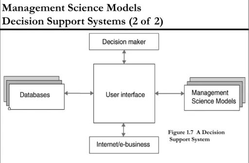
A decision support system is a computer-based system that helps decision makers address complex problems that cut across different parts of an organization and operations.
Features of Decision Support Systems
Interactive
Use databases & management science models
Address “what if” questions
Perform sensitivity analysis Examples include:
ERP – Enterprise Resource Planning OLAP – Online Analytical Processing
Copyright © 2010 Pearson Education, Inc. Publishing as Prentice Hall 1-30
Figure 1.7 A Decision Support System