不均勻系統中電漿與電磁波作用之理論解析與數值實驗

(1)

Resonance is a fundamental issue in science with wide applications and requires precise synchronization [4–7, 43]. For a harmonic oscillation with damping, the width of the frequency mismatch between the driving force and the oscillator is required to be smaller than the damping rate in order to remain in resonance [43]. For cyclotron resonance, the wave frequency has to be very close to the harmonic frequency of charge particle’s gyro-motion under magnetic field [1, 4–8]. Cyclotron instability through the resonance involving relativistic mass variation effect has been studied for half a century [1, 4–15, 35-36]. The cyclotron maser instability [4–7, 43] is the most important mechanism responsible for generating state-of-the -art high power microwave source with critical applications in space, defense, and industry. In order to drive the instability, it is well known [4–7, 43] that the precise synchronism has to be stably maintained and the frequency mismatch between the wave and the harmonic cyclotron frequency, _c, of the charge particles is required to be positive [4–7, 43]. While the charge particles are losing their kinetic energy to the wave, their Lorentz factor decreases, their harmonic cyclotron frequency increases, the frequency mismatch decreases, and thus the resonance is enhanced to sustain the wave growth and the instability [4–6].

Since they were first discovered, relativistic cyclotron instabilities [1–3]

have received much attention and found applications in many research fields such as radiation sources [4–9], fusion plasmas [10–15] and astronomy [16]. One of the most successful examples is electron cyclotron maser (ECM) which is unique as a powerful source to generate coherent radiation in millimeter and sub-millimeter regions. However, in order to maintain the resonance between wave and particles, the uniformity of the external magnetic field is always an important issue. For example, the typical variation of magnetic amplitude allowed in gyro-klystron, which is one of the ECM-based devices and widely used in radar applications, is within 0.1% [4]. Besides, as a well-known requirement being consistent with all theoretical studies and experimental observations [4], the frequency mismatch between the wave and the harmonic gyro-frequency of particles must be positive for driving relativistic cyclotron instabilities [4,6,17].

1.2 Background and current conditions

(4)

Energetic ions can be produced from fusion reactions; i.e. 3.5MeValpha particles from the reactions of a deuteron and a triton. The interaction between waves and energetic particles is an essential topic in the study of fusion plasmas for energy purposes [18–20]. Many instabilities can be driven by the energetic ions. Chen (1993) was the first to suggest the importance of the relativistic effect on the harmonic cyclotron instabilities driven by the energetic ions [12], although the Lorentz factor is very close to unity. This instability provides an explanation [21] for the ion cyclotron emission observed in JET [22–27] and is able to cause the selective gyro-broadening [28–31] or the anomalous thermalization [32] of the fast ions. The predicted result [30] of the selective gyro-broadening of the energetic alpha particles is found to agree well with the alpha energy spectrum measured in TFTR [33, 34]. However, in these works the relativistic mass effects were studied under the approximation of the magnetic field as uniform. Thus, it is reasonable to ask whether this instability can survive in the realistic fusion devices with a nonuniform magnetic field configuration. In fact, some people believe the relativistic mass variation should be a minor issue [35] and the phase synchronization in a resonance can be easily destroyed due to a nonuniformity [36]. If the instability can survive the nonuniformity of the magnetic field in fusion devices, the predicted consequences as discussed above should be seriously assessed for their implications and applications to fusion plasmas.

1.3 Research purpose

In this project, we will show the simulation and analytical results that impact our understanding of resonance and the requirement of frequency mismatch. In contrast to conventional wisdom [35], localized eigenmodes of cyclotron waves [44] are excited at the minimum of the magnetic field which is taken to be sinusoidal nonuniform. One of the possibilities is that resonance and the resultant structure of wave mode is a consequence of the need to drive instability for dissipating free energy and increasing the entropy. We even find that the wave mode can exist at where the wave eigenfrequency is lower than the local harmonic cyclotron frequency. An eigenmode theory derived is found to be consistent with the simulation results.

Both hybrid particle-in-cell simulations [37,38] and an analytical theory are developed to study the alpha-driven ion cyclotron instability and the resultant wave modes perpendicular to an external magnetic field whose magnitude varies

(5)

sinusoidally in the wave direction. The sinusoidal variation is employed here as a simple way to introduce nonuniformity in the magnetic field strength. A localized wave mode with a twin-wavelet profile driven by the alpha particles is observed around the minimum of the magnetic field even when the magnetic variation across the wave profile is much greater than the Lorentz factor minus one ( ! 1 = 9.4 × 10⁴ for a 3.5MeV alpha particle). Besides, the wave frequencies measured at different positions within the spatial extent of the wave mode are almost the same so that the wave mode observed should be an eigenmode. To investigate in depth the characteristics and the driving mechanism of the localized modes, an analytic theory based on expansion about an absolute instability condition [40] has been developed on the assumption that the magnetic field strength varies slowly. More specifically, the magnetic field strength considered in the theory is taken to be parabolic to approximate the magnetic field profile near its minimum used in the simulation. The eigenmodes predicted by the theory are found to agree well with those observed in the simulation including the wave profile, growth rate and frequency. It is interesting to note that the local wave frequency mismatch is negative at the two sides of the wave profile while positive at the center. The negative frequency mismatch result apparently violates the positive requirement of the cyclotron resonant condition [4] mentioned earlier. In addition, the magnetic variations within the extent of the twin-wavelet are 2.83×10³ and 2.97×10³ in simulation and theory, respectively, which are greater than the difference between the Lorentz factor of the alpha particles and unity. In section 1.4, the hybrid simulation and the localized wave modes observed will be studied. The analytical theory with a systematic expansion procedure to yield the solution and the behaviors of the eigenmodes corresponding to a weak magnetic nonuniformity are derived and discussed, comparing with the simulation results. Finally, section 1.5presents the discussions while the conclusion is given in same section.

1.4 Research method

1.4.1 Localized wave modes observed in the simulation with a nonuniform magnetic field

An electrostatic particle-in-cell-and-fluid hybrid code is developed to study the relativistic ion cyclotron instability (RICI). The simulation system is one-dimensional in the real space defined as the x direction and three-dimensional in the momentum space. In this code, the leapfrog method is

(6)

employed to advance system dynamics and solve the electric field from the Gauss law in k space. The fast ion species that can be strongly resonant with waves is treated with particle description, while the background ion species is simulated as fluid to considerably reduce the calculation. We consider the plasma consists of fusion-produced 3.5MeV energetic alphas ( ! = 1.00094) with an isotropic shell distribution in the momentum space, 5 keV thermal deuterons with a Maxwellian distribution and cold electrons in a background magnetic field B = B(x) ˆz . In thiswork, we take B(x) to be sinusoidal in order to simplify the simulation while retains the nonuniformity B(x) effects; that is, B = B0[1 + "!

sin(2#$%&'] with the uniform part of the magnetic field B0= 5 T and the magnetic nonuniformity parameter "!= 0.01 which presents the amplitude of the variation of external magnetic field. The L = 4096!x is the periodic system length, which is about 1.76m comparable to the minor radius of the fusion device. The cell size

!x is 0.043 cm which is subjected to the Courant condition to avoid potential numerical error when a finite time step !t = 0.025 is given. Besides, the simulation time is normalized to the relativistic cyclotron frequency of the alpha particle. Furthermore, the alpha density n₍ is 2×109 cm³, the deuterium density n_dis 1013 cm³and the electron density n_eis 1.0004 × 1013 cm³ for the charge neutrality. The energetic ions are simulated by the particle-in-cell method while the slow ions can be described by either the particle-in-cell or the fluid method and the electrons are approximated as a cold fluid. In the particle-in-cell method, we utilize a quiet-start technique [38] to reduce the numerical noise. For the fluid deuterium case, the number of simulation alpha particles is 10 077 696. In the case of simulation with particle deuterons, the number of alpha particles is 5038 848 and that of deuterons is 11 390 625.

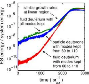
Figure 1 shows the histories of the electrostatic wave energy. Only the contribution of waves from spatial grid 2049 to 4096 is included in order to exhibit the unstable growth of the localized wave modes. The wave energy of the case with fluid deuterium and limited modes has the lowest initial noise level of 8×10¹¹and enters the exponential growth region at about t = 1000.

(7)

Figure 1. Histories of electrostatic wave (ES) energy for the cases of the fluid deuterium with

modes kept from 60 to 110, particle deuterons with mode kept from 60 to 110 and fluid deuterium with all modes kept, respectively.

With all modes kept, a higher noise level of 4 × 10⁹ is observed, but the growth rate at t = 2000 is similar to the previous case. For the particle deuterons case, the noise at the beginning is much higher than that of the fluid deuterium with the same modes. All three cases have a similar normalized growth rate of about 3 × 10³. In addition, they all saturate around t = 2500. Although, as we will see in section 3, the dominant modes observed in the simulation are around )*( 17 which means the )*D is about 0.9. Because the case of fluid deuterium with limited modes has the lowest noise level, and similar wave structures are obtained within the linearly exponential growth regime for particle or fluid deuterium, it is considered here as the typical case in the following discussions.

As observed in the simulations, the RICI is still able to survive the magnetic nonuniformity, even though the magnetic variation "!is much greater than the ! 1 of the alpha particles. Figure 2 presents the snapshots of the electrostatic field.

The spatial coordinate is normalized to the initial maximum gyro-radius of the alpha particles, *₍, and the origin corresponds to the minimum of magnetic field strength. Figures2(a) and (b) show a wave structure emerging from the noise as the instability enters the exponentially growing linear regime. Then, the distinctive wave mode of the twin-wavelet profile can be clearly observed in figures 2(c) and (d). Since the instability saturates around t = 2300, the

(8)

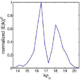
twin-wavelet structure changes as shown in figures 2(e)and(f). In addition, the k spectrum of the electrostatic field at t = 1900 during the linear regime is shown in figure 3, indicating two dominant peaks located at )*₍= 16 and 18, respectively.

It implies that this wave mode is constructed by a slow variation in its envelope accompanied with a fast oscillation inside.

Figure 2. Snapshots of the electrostatic field (in arbitrary units) at different times (a) t = 1500, (b) t

= 1700, (c) t = 1900, (d) t = 2100, (e) t = 2300 and (f ) t = 2500, respectively.

Figure 3. Snapshot of the electrostatic field in k space at the time t = 1900.

In simulations, the width of the twin-wavelet profile approximately reduces

(9)

from 11 to 7 *₍ as we increase the magnetic variation parameter, ", from 2×10³ to 6×10³; however, it does not appreciably tend to be more localized when the "!

continues to increase up to 1.2×10²in our simulation.

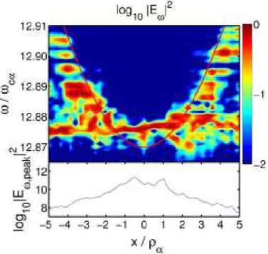
Figure 4shows the spatial frequency power spectrum as a function of x. The solid curve shows the local harmonic cyclotron frequency of the alpha particles.

It is interesting to note that the wave frequencies measured at different positions within the spatial extent of the twinwavelet have almost the same value, 12.875, indicating that the observed wave mode is an eigenmode. The frequency mismatch between the wave frequency and the harmonic cyclotron frequency is positive at the magnetic minimum. However, it is found to be negative away from the center by about two gyro-radii of the alpha particles. This negative frequency mismatch is against the well-known resonant condition of the relativistic cyclotron instabilities [4,6].

Figure 4. Normalized wave frequency power spectrum and amplitude in real space. The solid curve stands for the local harmonic cyclotron frequency of the alpha particles.

A previous work by Dong [39] also indicates that the instability can survive a nonuniform magnetic field and shows a localized wave mode. The corresponding characteristics and physics of the instability and the localized wave mode are, however, different from the present results. Dong employed a gyro-kinetic theory to derive an integral dispersion relation and solved it

(10)

numerically in k space. From his study, the eigenmode is localized as expected.

However, the corresponding eigenfrequency is significantly lower than the local harmonic cyclotron frequency of the alpha particles at the magnetic minimum;

that is, the resonant condition cannot be satisfied for driving a relativistic instability. Also, the localized wave mode has a different profile and may, as discussed in the following, correspond to different class of wave modes. From our simulations, we have observed not only the excitation of localized modes but also the convective waves which should decay rapidly when propagating away from the magnetic minimum. As a result, one possible explanation for the discrepancy between the results is that Dong’s mode is a convective instability while only modes satisfying the absolute instability condition can contribute to the existence of localized modes observed in the simulation. Thus, an analytical theory based on the absolute instability condition is needed in order to obtain correct results consistent with the simulation and to explain the characteristics and the interesting resonance physics relevant to the observed localized eigenmode.

1.4.2 Analytic study based on the absolute instability condition with a weakly magnetic nonuniformity

Consider the dispersion relation for a uniform magnetic field as D(+, k)=0 and for a nonuniform magnetic field as D(+, k, x)=0. Let "(x)= #$x)exp(ik x), where k represents the spatial fast-varying part of the wave function. By employing the two-scale-length expansions [40] with+=+ +"+, k= k i x, and x=x0+"x, the corresponding eigenmode equation becomes

where Q("+)= _!D"!# _!²D"!²/ 2 ...# higher orders; all terms are at +=+ , k=

k , and x=x₀.

To investigate the localized modes, we make a parabolic approximation of the magnetic field at the minimum as B(x)=B0[1+$b(x-x0)²/2], where $b denotes the nonuniformity; for the simulation case of " =0.01, $bis 3.71 10⁴. Choose

(11)

x₀=0 at the cell of 3072 for simplicity; all terms associated with the first order derivative to x₀will vanish.

We further request k_ satisfying the absolute instability condition of kD=0 [40], which implies that the group velocity is zero. Also, in order to remove the term related to _!²_kD, let #$x)= "(x)exp(ik₁x) and k₁=% _!²_kD/ _k²D"!. After some algebra, Eq. (1) can be transformed to a parabolic cylinder equation [41] as

Then, we obtain the eigenvalue of E=En=n+1/2 = Q("+)/(&² ²_kD) and the corresponding eigenfunction of "$t)="_n(t)=He_n(t)exp( t²/4), where &⁴ '

2 /

xD ²_kD, t '2^1/2&x, and the Hen(t) is the modified Hermite polynomial of order n, where the rank of the eigenvalue is n =0,1,2,.... During the algebra, we had also neglected the term of k which should be much smaller than the term of

2 2 2 2

( _!_kD) / _kD"! in Q("+) when the charge particlesstrongly resonate with the

wave. For localized solutions, "%should vanish while away from x0. Hence, only the solutions satisfying Re(t²) > 0 are chosen to make sure the localization.

The waves can propagate in both positive and negative x directions.

Therefore, with k₀ )k₍#k₁ , the wave function can be written as ,(x)="$x)[exp(ik0x)+exp( ik0x)] /2 ="$x)cos(k0x), which is a symmetric and localized solution.

To study the behavior of instabilities under nonuniform magnetic field, we use the dispersion relation derived for a uniform B [10, 11] and follow the procedures described above. From the dispersion relation D(+,k)=0, + can be determined from k numerically with Muller’s method. There are several solutions satisfying the* kD=0 condition; the mode with a highest growth rate is of interest.

The corresponding wave function is then calculated.

1.4.3 Comparison between the simulation and theoretical results

In this section, we try to extract some physical understanding by comparing

(12)

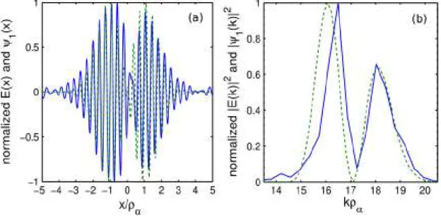
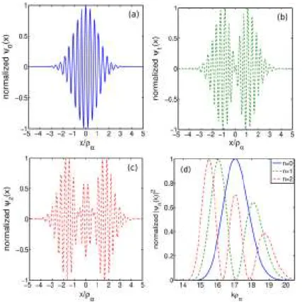
the simulation observations with the analytic results. As shown in figure 5, the twin-wavelet structure observed in the simulation is analogous to thewavefunction of the n = 1 eigenstate, &₁(x). Their spatial widths are both about eight gyroradii with two symmetric peaks located at one gyro-radius away from the center which corresponds to the magnetic minimum. In addition, both wave structures possess two peaks in the corresponding k spectrum. The dominant peak of the simulation twin-wavelet structure is at )*( = 16.5; slightly greater than that of &1(x) which is located around )*(= 16. However, their minor peaks in the k-spectrum coincide at )*( = 18.2. Meanwhile, the growth rate and wave frequency measured in the simulation for the twinwavelet structure are 3×10³ and 12.875, respectively; to be comparable to 2.54×10³ and 12.871 predicted for the n = 1 eigenstate.

Figure 5. Comparison of wave structures in the real space (a) and in the k space (b) from the simulation at t = 1900 (solid) and the theory of n = 1 (dashed).

Furthermore, by examining the k spectrum for the different eigenstates as shown in figure 6, and making a judicious choice in the k-spectrum filtering, it is possible for us to only excite the n = 0 eigenstate with the other eigenstate suppressed. For example, we have limited the modes kept in simulation from 85 to 95 (i.e. )*( = 16.29 to 18.21). In this case, the instability starts to grow exponentially at t = 1600 and saturates at t = 3000. A single wave packet forms during the linear regime as shown in figure 7. The width of this packet is about 6

*(; which is slightly wider than that predicted for the n = 0 eigenstate. However, both k spectra have similar profiles and both peak at )*( = 17.24. Additionally,

(13)

the growth rate of this wave packet is 3.8 × 10³ which also agrees with 3.2 × 10³of the n = 0 eigenstate.

Figure 6. Eigenfunctions of different eigenstate ranks: (a) n = 0 (soild), (b) n = 1 (dashed), (c) n = 2 (dashed and dotted) in the real space and (d) the k space.

Figure 7. Comparison ofwave structures in the real space (a) and in the k space (b) from simulation at t = 2200 (solid) and theory of n = 0 (dashed).

Thus, the simulation results agree well with the theoretical predictions and

(14)

clearly indicate that the localized modes observed in the simulations are the bounded eigenstates trapped by the potential well due to magnetic field nonuniformity. This explains the spatial independence of the wave frequency measured within the spatial extent of the twin-wavelet structure. In addition, the convective waves have not been observed because they asymptotically decay in time as it propagates away from the local unstable domain to the stable domain [42]. Although the theory should only be considered as qualitative in the limit of high magnetic nonuniformity used in simulations, it still demonstrates an amazing degree of consistency with the simulation.

1.5 Discussion and conclusion

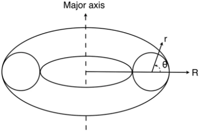
The magnetic field in a realistic device is not uniform. For example, in a tokamak whose corresponding schematic plot is shown in the figure 8, the toroidal magnetic field in low--! plasma can be approximately written as B_. [B0[1 (r/R) cos /]; where r andR are the minor and major radii, respectively, and /!is the poloidal angle. Thus, the variation of its magnetic field is sinusoidal in the poloidal direction and the magnetic field strength approximately decreases with the increase in its major radial position. When the directions of both the wave and the magnetic field nonuniformity are along the direction of the major radius, the decrease in magnetic field may be reversed in a high--! and/or steep pressure gradient device. To balance the pressure force, the magnetic field may be increased so much that its slope becomes positive locally along the major radial direction. Thus, a local parabolic well of the magnetic field profile as studied in the analytic theory may be regarded as an approximation around the magnetic field minimum. On the other hand, when both directions are along the poloidal direction, one may find a magnetic profile with a sinusoidal nonuniformity. However, the Doppler shift effect of the alpha particles should be accessed while the velocity of slow ions is too small and the electron cyclotron frequency is too high. The resonance condition is given as +!– k||v_|| 0+1(. The Doppler shift effect is related to k_||v_||, where k_|| = m/(qR), m is the poloidal mode number and q is the safety factor while the cyclotron resonance is related to +!

0+₁₍. For m = 1, q = 3, R = 6m and other parameters used in this paper, the resonance ratio is k_||v_||%2+! 0+₁₍) ~ 0.933, where the velocity ratio is 3!= v_||/v䎹. The resonance ratio becomes smaller when the resonance harmonic number is higher such as in a higher -! plasma. For an alpha particle with a large velocity ratio and thus a larger resonance ratio, it may be involved in driving instability instead via Landau growth, whose growth rate is proportional to the particle

(15)

density. For that with a small velocity ratio and thus a smaller resonance ratio, it may still remain in the resonance for driving the RICI whose growth rate is proportional to the square root of the particle density. Note that the RICI is selective and only the alpha particles with a high perpendicular velocity (e.g. a small velocity ratio) are involved in the interaction with the wave [28–31].

Because the instability and resultant selective broadening can survive under the simplified nonuniformities, their consequences (e.g. on driving waves each occupying a space of a fraction of the minor radius as well as on significantly changing the perpendicular velocity and the pitch angle of energetic alpha particles) and implications (e.g. channeling the alpha particles energy and/or modifications in the particle orbits) for fusion plasmas deserve to be further studied.

Figure 8. A schematic plot of a tokamak device; the r and R are the minor and major radii, respectively, and /!represents the poloidal angle.

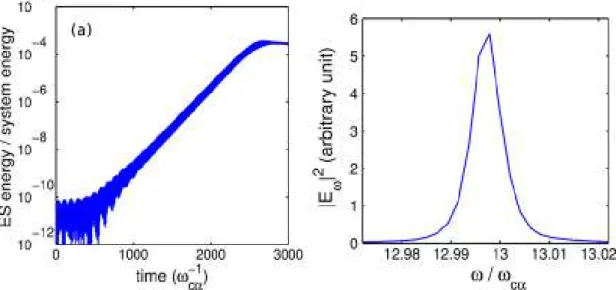
In figure 9, we show the growth rate and the real frequency versus )*(based on the local dispersion relation, equation (9), at x = 0; i.e. under a uniform magnetic field. It clearly shows that, for some unstable modes, the wave frequency can be lower than the harmonic ion cyclotron frequency [12] which apparently violates the positive requirement of the frequency mismatch. Although they are not the most unstable mode, as long as one of them can satisfy the absolute instability condition while the most unstable mode cannot, it can survive the convective damping due to the nonuniformity of the magnetic field. Thus, the localized mode can be excited and retains the characteristics of the survivable mode. Moreover, we have also run a simulation keeping only the mode of )*₍ = 17.25; which is close to the mode satisfying the absolute instability condition considered earlier. Figure 10 shows the instability can indeed exist with a

(16)

normalized growth rate and frequency mismatch at 3.7 × 10³ and 2 × 10³, respectively, which agree well with the theoretical predictions. Thus, even in a uniform plasma, the electrostatic cyclotron instabilities may not be constrained by the requirement of a positive frequency mismatch. While the relativistic cyclotron instability studied here is for energetic ions, the findings may still have important implications and thus applications for electrons. For relativistic electron cyclotron instabilities, it is well known that the frequency mismatch is required to be positive. The devices usually have a fixed magnetic field. Its operation frequency is determined by the magnetic field and the frequency mismatch. If it is possible to operate for both positive and negative mismatch, the tunability of the devices may be increased.

Figure 9. The normalized growth rate (solid) and the frequency mismatch between wave and resonant cyclotron harmonic (dashed) in a uniform magnetic field.

The RICI under sinusoidal nonuniform magnetic fields has been investigated via, respectively, simulation and analytic methods, adopting a parabolic magnetic field approximation. Other types of nonuniformity for fusion plasmas deserve further investigation. In the simulation, we use the particle-in-cell method to describe the alpha particles and consider the deuterium as a fluid to obtain results with high resolution. Localized wave eigenmodes are observed at the magnetic minimum when the external magnetic field has a sinusoidal nonuniformity. The spatial structure of the electrostatic wave looks like a twin-wavelet. In order to understand the physics and mechanism involved, an analytic theory based on

(17)

expansion around the absolute instability condition has been developed. The parabolic magnetic profile considered in theory is an approximation for the magnetic minimum employed in the simulation. Bounded eigenstates are found at the magnetic minimum as observed in the simulation. The structure, growth rate and frequency of the theoretical n = 1 eigenstate are in good agreement with the simulation twin-wavelet. On the other hand, the n = 0 eigenstate of a single packet wave mode from the theory is verified by another simulation; with more limited modes kept in the simulation, only the wave mode of a single packet can be excited, which corresponds to the n = 0 eigenstate. In contrast to the conventional requirement of a positive frequency mismatch, the instability can drive the unstable wave mode existing where the frequency mismatch is negative.

In addition to possible applications to fusion plasmas, this study may also be helpful for electron cyclotron instability and application, especially for high harmonic and for tunability. These results have been published [81-82].

Figure 10. The growth of instability (a) and the measured frequency power spectrum (b) when only one mode )*(= 17.25 is kept in the simulation.

(18)

2 The interaction between surface plasmon polaritons and electromagnetic wave in subwavelength nano-structures

Diffraction, as a general wave phenomenon which occurs whenever a traveling wave front encounters and propagates past an obstruction, was first referenced in the work of Leonardo da Vinci in the 1400s [45] and has being accurately described since Francesco Grimaldi in the 1600s [45]. Explanation based on the wave theory was not available until the 1800s [45]. The diffraction limit was the inspiration for Heisenberg’s quantum uncertainty principle [46,47]

that is a foundation of modern science; in fact, they can be deduced from each other [46-48]. The diffraction sets the smallest achievable line width or spot size [1-4], which is the ultimate manipulability and resolution [45,48] of numerous diagnostic and fabrication instruments. For a single aperture, the limitation can be given as +,/NA, where , is the wavelength in vacuum, NA = n sin- ฀ŪŴġ ŵũŦġ ůŶŮŦųŪŤŢŭġ aperture฀฀n is the refractive index of the medium where the focused light locates, -*is the convergence angle of the light, and the constant + is 0.38, 0.5 and 0.61 for a ring, line, and circular aperture, respectively [45].

The diffraction limit concerns travelling light that can propagate freely in the free space, in contrast to the evanescent near-field [49,50] that is electrostatic [51-56] or magnetostatic [57,58], needs a preferred plane or surface for propagation and cannot propagate freely in the free space, such as occurs in a super lens [51-58]. For a dipole source, the near, intermediate (or mid) and far fields decrease away from the source as proportional to 1/r³, 1/r²and 1/r, respectively [76], where r is the distance; for a line source, the far field is proportional to 1/r^1/2. The scaling laws of the far field conserve the field energy. Mathematically, the divergence of the electrostatic field and the Laplacian of the scalar potential are determined by the charge density according to Gauss’s law and Poisson’s equation, respectively, while the fields of propagating light concerned with the diffraction limit are decided by the spatial curl and temporal derivative equations (i.e., Faraday’s and modified Ampere’s equations) involving the scale of wavelength.

Thus, a new understanding and a different approach are needed to produce a beyond-the-limit focusing of travelling light.

(19)

Both the theory of the conventional diffraction limit of light and the Heisenberg’s quantum uncertainty principle consider wave function expanded into reciprocal space and a situation where the scale of the eigenfunction is half the wavelength or larger. For quantum mechanics, the surface integral involving the wave function is assumed to vanish when taken over a very large surface or an infinite potential well. For the latter, the spatial eigenvalue (i.e., the wave number) is k = m./a, where m is a natural number (i.e., non-zero) and a is the well width.

For the ground state, the well width is half a wavelength, while the wave function is the corresponding harmonic function.

The excitations of surface plasmon [59-61] on metallic surfaces and surface-plasmon-like modes [62-63] are claimed to enhance [64-65] the transmission of light and to beam/focus [66-68] it through subwavelength holes/slits [69]. In fact, the light and the surface plasma are coupled and hence are self-consistent within the slit. The wave function across the slit is close to a constant and drops sharply on the surface. This kind of function with k = 0 mode bounded within a sub-limit scale is not considered in the conventional theories and thus is not within their scope.

The innovative approach and physical mechanisms of the focusing aperture beyond the conventional diffraction limited line width (FAB) of half the wavelength [70] are demonstrated here with the FAB lens including a metallic film with a double-slit and a patterned exit structure, as shown in Fig. 11(a). The width of each slit is smaller than half the wavelength, and thus the limited line width. At the same time, the width of the central metal strip (the interslit spacing) is about a half-wavelength that gives rise to a half-wavelength dipole antenna which can effectively emit propagating fields. Besides the generation of sub-limit wave functions within the slits and at the central area resulted from a polarized field conversion and the surface current, the transmitted light of sub-limit scale will be shown to be bent toward the center and focused to achieve a lower diffraction limit.

Finite-Difference-Time-Domain (FDTD) simulation [71] is employed to verify the approach. A structured thin silver film with 20 and 2 grooves at the incident and exit sides, respectively, as shown in Fig. 11(b)is employed as our FAB lens. A simplified structure on silica substrate has been employed in an optical

(20)

experiment [72] that verifies this approach, in addition to another experimental confirmation in the microwave range.The refractive index of silver [73] used for ,

= 633 nm is 0.134 + i 3.99. The system has 1600 × 1000 cells of the Yee space lattice with a unit cell size of 5 nm. The top of the silver film is at the y = 800 cell.

The time, t, is normalized to the light period, and the time step is 0.005.

Figure 11(c) shows a snapshot of the magnetic field indicating the propagation of the focused light to the far zone and the near field along the surface.

As shown on Fig. 1(d), the Hzfield is almost in phase with the Exfield, except near the surface at y = 0.2 /m. Also, the profile fits better with the scaling of a far field than that of a mid or near field. Thus, the focused fields are dominated by the propagating field.

For better understanding of the approach and the physics involved, let us consider the dynamics of the focusing. The plane wave propagating downward is transmitted through the double-slit being enhanced by surface plasma and split into

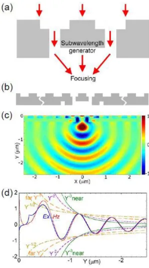
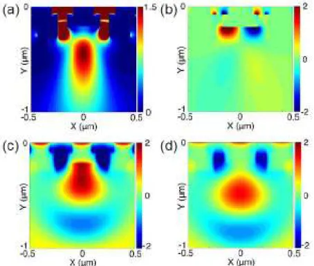
Fig. 11 The schematic structure of the aperture, the approach and the simulation result. (a) Schematic diagram of the approach, aperture structure and the paths of the light transmitted, bent and focused, including the generator of sub-limit wave function at the central area. (b) The schematic structure of the aperture on a silver film used in the FDTD simulation. The depth, the width and the distance in between of the periodical grooves at the incident side are 80 nm, 200 nm and 200 nm, respectively; the slit width is 80 nm; both the width and depth of grooves at the exit side is 80 nm; the distance between the slit and the exit groove is 160 nm;

the film thickness is 280 nm; the thickness and the width of the central strip are 200 nm and 320 nm, respectively. In order to clarify the possible near-field involvement, the central metal width of 320 nm and the exit width of 480 nm are larger than half the wavelength, 316.5 nm. (c) The snapshot of the Hzfield at t = tf+ 0.12, where tfis defined later. (d) The y profile of the Hz[in (c)] and Exfields and the estimated curves of the profile peaks, normalized to the peak at y=-1.175, as a function proportional to y^-1/2(brown long dashes and dashes) and to y^-1, y^-2 and y^-3 (orange long dashes, purple dashes, green dots) for the fields being the far, mid and near fields, respectively, according to a dipole source model [32].

(21)

two beams which are bent toward the symmetry (y-) axis. In addition, due to the surface currents the metal strip between the slits acts like a half-wavelength dipole antenna (a generator). The interference of the diffracted wave functions from the bent beams and that of the generator result in the subwavelength focal spot, as indicated by the time-averaged E_x field energy contour plot shown in Fig. 12(a).

The Ey field, the polarized surface charge and the x component of time-averaged Poynting vector of the diffracted light from one slit, shown on Fig. 12(b), are cancelled with those from the other. The cancellation converts the energy of the polarized surface charge and the Eyfield to increase the focused Hzfield [Fig. 12(c), at the time (and the phase) defined as t = tf] and hence explains the behavior of the Exfield (Fig. 12a) at the central region so as to generate a sub-limit wave function there. The overall line width of the focused field can be further squeezed by the diffracted field, which is focused at a time half of the period earlier than the focused field, connecting with the transmitting field, which is focused at a time half of the period later, as shown in Fig. 12(c-d). In order to form this field connection,

there is a requirement on the width of the central metal strip and the field diffraction has to be slowed down by the surface plasma including the effect of the grooves on the structure. The snapshot of the focused Hzfield (Fig. 12c) is taken at the moment that there is a peak of focused positive magnetic field outside the

Fig. 2 The contour plots of the fields. (a) The time-averaged contours of the Exenergy. (b) The time-averaged contours of the Poynting vector in the x direction. (c) The snapshot of the focused Hzfield at t = tf. (d) The enlarged snapshot of the Hzfield at t = tf+ 0.12. All are normalized to the incident light.

(22)

surface and near the peak position of the time-averaged Poynting vector in the original y propagation direction shown later in Fig. 14(a). After being focused at t

= t_f, the light diffracts to forward angles, and the H_zfield propagates out while it is still squeezed as shown in Fig. 12(d). Then, the focused light propagates out to the far zone, as also evidenced from the movies of the electric and magnetic fields.

The line width of the focused light can be defined by the full-width-half-maximum (FWHM) or the width of the spot of the Hzenergy averaged-along-x as twice the position uncertainty that is defined as x = (<x²>-<x>²)^1/2, where <f> ='Hz2

f dx / Hz2

dx. Figure 13(a)shows that the FWHM of the time-averaged Hzfield energy agrees well with that for the snapshot of Hzfield energies. While the peak intensity of the focused light remains to be higher than that of the incident light, the FWHMs at the normalized distance kr up to 4.17 is smaller than the diffraction limited line width of half the wavelength. The x profiles of the peak focused light at three different times/phases are shown in Fig. 13(b). At the time t = tf, FWHM is 0.286 while the width is 0.217 when averaged over the focused line; it is !"#$!% when averaged over the profile. The FWHM becomes 0.394% %at the time of 0.12 period later and 0.498 %at the time of t = tf+ 0.29 while the peak of the focused light has reached at a distance of 0.664 %away from the surface. All the widths discussed above are smaller than the diffraction limited line width of half the wavelength. Obviously, the diffraction limit has been locally overcome by a result at the intermediate zone in which there is such a small single-line width occurring with regard to the focused light.

For a far (near) field [32], the electric field is in phase (out of phase) with the magnetic field so that the Poynting vector (i.e., the energy flow) is not (is) zero.

Fig. 13 The profiles and the width of the focused light. (a) The FWHM vs. normalized r profiles of the snapshot of the Hzfield energy (blue squares) and the time-averaged Hzfield energy (red curve), where r is the y distance from the metal surface. (b) The profiles of the focused Hzfield energy at t = tf(red curve), tf+ 0.12 (blue dashes) and tf+ 0.29 (green dots).

(23)

The focused light beyond the diffraction limited line width of half the wavelength is located at the intermediate zone [74]. To characterize it further, the time-averaged Poynting vector in the original y propagation direction shown in Fig.

14(a)also indicates that the focused fields are propagating and hence are capable of travelling to the far zone [74]. As a travelling light is an indicator of the capability of our approach for moving the focal point away from the surface, this makes the FAB lens superior to evanescent near-field solutions [49-58] for many critical applications.

The involvement of the near field on the line width of the focused light is quantitatively investigated in-depth. At the middle location of the central metal strip surface, the magnetic field is out of phase with the electric field and in phase

Fig. 14 The Poynting vector contours and the field profiles. (a) The time-averaged contours of the Poynting vector (i.e., the energy flow) in the y direction. (b) The temporal profiles of the magnetic field Hz(red curve), the electric field Ex(blue dashes) and the current Jx(green dots) at x = 0 of the central metal surface. (c) The x profiles of peak Ex(blue dashes) and ZHz(red curve) fields at t = tf

+ 0.12; where |Z| = 0.832 and the phase is 3 cells or 0.0237 wavelength. (d) The r profiles of the Ex

field at t = tf(light blue short dashes), t = tf+ 0.13 (blue dashes), and t = tf+ 0.29 (purple short dashes and dashes) when the FWHM of the Hzenergy is still smaller than half the wavelength, as well as the ZHzfield (red curve; the estimated far Exfield; where |Z| = 0.840), the near Exfield (dark green dots;

the difference of the overall and far fields), and the near Ex field for the case of an almost perfect electric conductor (light green dots and short dashes).

(24)

with the surface current -J_x, as shown in Fig. 14(b). Thus, it is dominated by the near field. But, at the time of t = t_f + 0.12, the focused light has moved out. Its magnetic field near the surface is close to zero on average and is a small positive number at the middle. The focused E_x field has a similar contour as the H_zfield.

The ratio and locations of their peaks determines the impedance Z. The estimated far Ex field is ZHzthat agrees well with the measured Ex as shown in Fig. 14(c).

This is one more indication [76] for the focused light to be dominated by the radiative field, as also evidenced by the propagation of the Ex field at different times shown in Fig. 14(d). At the time 0.01 later, the magnetic field at the middle of the central metal strip has dropped to a negative value very close to zero. As shown in Fig. 14(d), the estimated far Ex field along kr based on the analytical theory is in good agreement with the focused field obtained from the simulation.

The near Exfield including the intermediate field resultsfrom their difference and is decreasing away from the surface as expected with the length of half the field energy being kr = 0.476 or less than 0.1; that is consistent with the length scale of the near zone measured by NSOM [76-76]. The near field is smaller than the far field at kr > 1. Although the mid field may not be completely ignored because of the small phase difference (see Fig. 11(d), Fig. 14(c)); the effect of the near field is negligible at the intermediate zone of 2 < kr < 4, where the line width of the focused light is smaller than the diffraction limited value. Since the near field is expected to be caused by the plasma effect on the metal surface, we also calculate the near field for the case of an almost perfect electric conductor whose plasma frequency is given as ten times that of the silver. The result confirms that the near field is negligible in our focusing.

2.5 Summary and conclusion

Being able to achieve a lower diffraction limit, the focusing of light is intellectually intriguing and important for application possibilities. It may be employed to manipulate and image biomolecules at a higher precision, resolution and depth of focus with propagating light, to sense the structure and dynamics of biological and physical systems at a smaller scale, to diagnose and modify material surfaces with greater precision. In addition, it allows to remove the limit on photolithography, which is the key issue preventing the further progress of the semiconductor industry according to Moore’s Law, to craft finer circuits, to produce and read smaller spots for optical storage, to focus light for optical detection/imaging and into photonic and plasmonic circuits [77],to connect optical

(25)

systems and finer electronic circuits, among many others. The physical mechanisms might be used in applications required for the processing of optical information and thus in communication and optical computing processes.

In summary, the physical mechanisms of the innovative approach using a miniature FAB lens are demonstrated to focus light to a single-line with its width smaller than the conventional diffraction limited value in the intermediate zone of 2 < kr < 4. It is quantitatively verified that the involvement of near-field in the focused fields is negligible. As of result of being able to propagate light, this scheme can be superior to those based on the involvement of the near-field.

Besides the academic interest generated by the physical mechanisms and the approach, the light focusing process is expected to open up a wide range of application possibilities, especially with regard to the capabilities of the focused light being able to propagate, tuning the focal point position and reducing the sizes of the focused light spot and the corresponding devices. The result has been accepted to be published [83]

(26)

3 Strategy for designing epsilon-near-zero nanostructured metamaterials over a frequency range

Epsilon-near-zero (ENZ) materials may be used as optical “insulators” for the displacement currents in optical nanocircuits, improving the directivity of antennas and transmission efficiency of waveguides with sharp bends, far-field subdiffraction optical microscopy, tailoring the wave front of arbitrary light sources, the transmission of subwavelength Gaussian beams, etc [78].

Dealing with a single frequency limits the possibilities for a practical implementation of ENZ metamaterials. Nevertheless, so far nobody has designed such materials ensuring the low permittivity over a frequency range. It is well-!"#$"%&'(&%)&%)*%+(*,%&#%-./-)//%&'+%0#"1)&)#"%2 0 at a frequency of interest using a composite with layered or filament geometry. Using effective medium theory we show that the same condition can be fulfilled over a frequency range and develop our concept for designing broadband ENZ metamaterials.

Consider a composite made of parallel layers (see Figure 15). Each layer has its own permittivity i.The volume fraction of the ith layer is fi; the applied electric field is normal to the layer interfaces. Because the normal component of the displacement is continuous at the boundaries, the effective permittivity of the composite effmay be written as the harmonic average,

FIG. 15. Schematic of the composite: the unit cell consisting of 7 parallel layers.

(27)

1

eff i fi i

&^' (

)

& . (3)

If now _i =0 for any layer then _eff =0 for the whole composite. Having closely located zeros of _iin a frequency range, we get the condition _eff_eff 0 over the range.

How to obtain zeros of i? Many mixing rules allow it for two-phase composites with properly chosen parameters. So, we could design each layer in the form of metal cylinders with the permittivity m and filling factor fim inside a dielectric with the permittivity d and filling factor fid, or could consider parallel cylindrical holes inside a metal. In both cases the applied electric field is directed along the dielectric/metal interfaces, and the permittivity of each ith layer is the arithmetic average,

id d im m

i f f

& ( & * &

(4)

where f_id=1-f_im. Then, the condition _i= 0 is fulfilled if f_id = _m/( _m- _d) and f_im =

d/( _d- _m).

Let a composite consist of unit cells, each of them consists of 11 parallel layers and fi= 1/11 (the layers are of uniform thickness). To null the permittivity in the range 650 nm – 750 nm, we could design the layers with i =0 at regularly spaced wavelengths 650, 660, …, 750 nm, so that the interval !"between adjacent nulled wavelengths is 10 nm. To null the permittivity in the range 675 nm – 725 nm, the interval is 5 nm. To null the permittivity in the range 685 nm – 715 nm, the interval is 3 nm. Furthermore, let d=1.8 and silver with a frequency-dependent permittivity &_m (&_m+ *i&_m++ be a metal phase. Having found fid and fim at the corresponding frequencies, one gets eff from Eqs. (3) and (4). Using the Drude model for silver, we calculated _eff(see Figure 16). Actually, | _eff | is small in the considered ranges, but Re( _eff) passes through zero at the only wavelength close to the range center (700 nm). Thus, more complicated structure should be used to ensure the condition Re( _eff)34%#5+6%&'+%6("7+8

(28)

FIG. 16. Spectra of | eff|, Re( eff), and Im( eff) for nanocomposites with different intervals between adjacent nulled frequencies.

Generally, Re( _eff) may be arbitrarily close to zero over a frequency range.

Formally, the problem reduces to minimizing the objective function

, -

1

Re ;

M

eff fi d

.

. & . .

/

where the factors fi are fitting parameters. The objective function in the form of the mean square deviation from zero may be also chosen.

The numerical solution of the problem is a standard mathematical procedure and presents few difficulties.

Schematically, two possible geometries of the composite can be represented as in Figure17.

FIG. 17. Possible geometries of composites under consideration.

(29)

The first geometry may be imagined as a forest of metal wires of varied width inside a dielectric or, alternatively, an array of dielectric channels of varied width inside a metal. For the circular wires, the metal filling factor in the ith layer, f_im, may be related to the corresponding radius, r_i, via f_im=#$%_i², where N is the wire concentration.In the case of the circular channels, the dielectric filling factor in the ith layer fid = 1- fim= #$%i2

. The other geometry is an array of parallel channels of varied length. For cylindrical metal channels of equal width, the metal filling factor in the ith layer fim= Ni$%². The thickness of the ith layer ti=fih, where h is the total thickness of the cell.

For demonstration, consider nulling Re eff9:;%)"%three ranges with the spectral

$)1&'*% <44=% >44% ("1% ?44% "@% 0+"&+6+1% (&% ABCC4% "@% 9*++% D)7.6+%18). For the narrowest range 500 nm – 600 nm, breaking the range into ten intervals (!_A= 10 nm) and fitting the parameters fi yield |Re eff9:;EF4844C%)"*)1+%&'+%G("d 512-581 nm.

For the range 450 nm – 650 nm (!A= 20 nm) one gets oscillating Re eff9:;%$)&'%&'+%

oscillation amplitude less than 0.02 inside the band 475-625 nm. For the widest range 400 nm – 700 nm, breaking the range into twenty intervals (!_A= 15 nm) and fitting the parameters f_iyield oscillating Re _eff9:;%$)&'%&'+%#*0)//(&)#"%(@H/)&.1+%"#&%

exceeding 0.008 inside the band 415-675 nm.

FIG. 188% IH+0&6(% J+92eff) for nanocomposites with different intervals between adjacent nulled frequencies.

Our results show how to improve the efficiency of nulling. As the effective medium approximation is valid, even for a range as wide as desired, it is possible to

(30)

get Re _eff(&) arbitrarily close to zero by enlarging the number of the cell layers. The optimum number of the layers depends on how drastically the permittivity changes within the range.

3.5 Summary and conclusion

We have, for the first time, proposed a general technique for designing broadband ENZ metamaterials using the effective medium theory. Yet, it is a crude approximation, and we feel a need for a more sophisticated technique. If the losses are small, the dielectric response of ENZ metamaterials can become nonlocal [79];

we hope to address this issue in our future work. We have considered only one specific geometry and may not claim that it is the best one.

ENZ metamaterials considered above are anisotropic like single axis crystals.

In many cases, however, this is not a critical issue, for example, when dealing with far-field optical microscopy, directive emission in metamaterials, or cloaking techniques based on the scattering cancellation [80]. This result have been published [84]

(31)

4 References

[1]. Twiss R Q 1958 Aust. J. Phys. 11 564

[2]. Schneider J 1959 Phys. Rev. Lett. 2 504

[3]. Bekefi G, Hirschfiled J L and Brown S C 1961 Phys. Rev. 122 1037

[4]. Chu K R 2004 Rev. Mod. Phys. 76 489, and references therein

[5]. Chen K R, Dawson J M, Lin A T and Katsouleas T 1991 Phys. Fluids B 3 1270

[6]. Chu K R 1981 J. Chin. Inst. Eng. 4 85

[7]. Chu K R and HirshÞeld J L 1978 Phys. Fluids 21 461

[8]. Chen K R and Chu K R 1986 IEEE Trans. Microw. Theory Tech. 34 72

[9]. Chen L et al 1988 Phys. Fluids 31 3116

[10]. Chen K R 2000 Phys. Plasmas 7 844

[12]. Chen K R 1993 Phys. Lett. A 181 308

[14]. Chen K R et al 2005 Phys. Rev. E 71 036410

[15]. Chen K R, Chen H K and Lee S H 2007 Phys. Plasmas 14 092102

[16]. Wu C S and Lee L C 1979 Astrophys. J. 230 621

[17]. Cartier S L, D’Angelo N and Merlino R L 1985 Phys. Fluids 28 3066

[18]. Furth H P et al 1990 Nucl. Fusion 30 1799

[19]. Fisch N J and Rax J M 1992 Phys. Rev. Lett. 69 612

(32)

[20]. Valeo E J and Fisch N J 1994 Phys. Rev. Lett. 73 3536

[21]. Chen K R, Horton W and Van Dam J W 1994 Phys. Plasmas 1 1195

[22]. Cottrell G A and Dendy R O 1988 Phys. Rev. Lett. 60 33

[23]. Dendy R O, Lashmore-Davies C N and Kam K F 1992 Phys. Fluids B 4 3996

[24]. Coppi B 1993 Phys. Lett. A 172 439

[25]. Dendy R O et al 1994 Phys. Scr. T 52 135

[26]. Fulop T et al 1997 Nucl. Fusion 37 1281

[27]. McClements K G, Hunt C, Dendy R O and Cottrell G A 1999 Phys. Rev.

Lett. 82 2099

[28]. Chen K R 1995 Nucl. Fusion 35 1769

[30]. Chen K R and Tsai T H 2005 Phys. Plasmas 12 122510

[32]. Chen K R 1994 Phys. Rev. Lett. 72 3534

[33]. Medley S S et al 1996 Rev. Sci. Instrum. 67 3122

[34]. Medley S S et al 1996 Plasma Phys. Control. Fusion 38 1779

[35]. Fruchtman A, Fisch N J and Valeo E J 1997 Phys. Plasmas 4 138

[36]. Istomin Y A 1994 Plasma Phys. Control. Fusion 36 1081

[37]. Dawson J M 1983 Rev. Mod. Phys. 55 403

[38]. Birsall C K and Langdon A B 1991 Plasma Physics via Computer Simulation (New York: Hilger) p 394

(33)

[39]. Dong J Q 2005 Plasma Phys. Control. Fusion 47 1229

[40]. Chen L 1987 Waves and instabilities in plasmas (Singapore: World Scientific) p 4, 31

[41]. Abramowitz M and Stegun I A 1972 Handbook of Mathematical Functions with Formulas, Graphs, and Mathematical Tables (National Bureau of Standards Applied Mathematics Series 55) (New York: Dover Publications) p 686

[42]. Lashmore-Davies C N and Dendy R O 1989 Phys. Rev. Lett. 62 1982

[43]. R. P. Feynman, R. B. Leighton, and M. Sands, The Feynman Lectures on Physics Mainly Mechanics, Radiation, and Heat (Addison-Wesley Publishing, Reading, MA, 1968), pp. 23–24

[44]. K. R. Chen, Bull. Am. Phys. Soc. 45(7), 132 (2000)

[45]. M. Born and E. Wolf, Principles of Optics, (Pergamon, Oxford, 2005).

[46]. W. Heisenberg, The Physical Principles of the Quantum Theory, (University of Chicago Press, Chicago, 1930).

[47]. R. P. Feynman, The Feynman Lectures on Physics, (Addison-Wesley, Redwood City, California, 1989).

[48]. F. J. Duarte, Tunable Laser Optics, (Academic Press, Amsterdam, 2003).

[49]. M. A. Paesler and P. J. Moyer, Near-Field Optics: Theory, Instrumentation, and Applications, (John Wiley, New York, 1996).

[50]. S. Kawata (Ed.), Near-Field Optics and Surface Plasmon Polaritons, (Springer, Berlin, 2001).

[51]. J. B. Pendry, Phys. Rev. Lett. 85, 3966 (2000).

[52]. X. Zhang and Z. Liu, Nature Mater. 7, 435 (2008).

[53]. N. Fang, H. Lee, C. Sun, X. Zhang, Science 308, 534 (2005).

不均勻系統中電漿與電磁波作用之理論解析與數值實驗

Contents

)

/