整合多重隨機奇異值分解與理論分析

國⽴臺灣⼤學理學院應⽤數學科學研究所 碩⼠論⽂

Institute of Applied Mathematical Sciences College of Science

National Taiwan University Master Thesis

整合多重隨機奇異值分解與理論分析

Theoretical and Performance Analysis for Integrated Randomized Singular Value Decomposition

張⼤衛 Da-Wei Chang

指導教授 王偉仲博⼠

Advisor: Weichung Wang, Ph.D.

中華民國 106 年 7 ⽉

July, 2017

ii

doi:10.6342/NTU201702973

iv

doi:10.6342/NTU201702973

誌謝

在最⼀開始 我想感謝與這篇論⽂相關的所有⼈ 沒有你們的協 助 我無法將這篇論⽂完成

感謝我的指導教授王偉仲⽼師 教導我該如何進⾏研究 定期開會 討論進度 平常也總是開著辦公室的⾨ 當遭遇問題 或是有新的進 展時 都可以⼀起討論 並給予建設性的回應 除了學術討論以外 也對寫作與報告的模式進⾏指導 讓我對於論⽂的寫作有更深⼊的認 識 感謝中研院統計所陳素雲⽼師與陳定⽴⽼師讓我參與整合隨機奇 異值分解的這項研究 並且在理論⽅⾯提供指導與協助 感謝我的同 學楊慕與林建燿 陪伴我⼀起討論 並且提出了許多新的點⼦與想法 感謝 R439 研究室的所有同學 營造出歡樂的研究氣氛 推動研究的推 展 並且舒緩了研究不順利時的煩躁感 感謝我的家⼈在這段時間裡 在⽣活與⼼理上的⽀持 使我可以無憂無慮 專⼼⼀致地完成這篇論

⽂

最後 再次感謝所有與這篇論⽂相關的所有⼈ 從⼀開始接觸問 題 到現在完成這份論⽂ 因為有敬愛的師⾧ 同學與家⾧的⽀持 才能讓這篇論⽂順利誕⽣

vi

doi:10.6342/NTU201702973

Acknowledgements

First of all, I would like to thank my advisor Professor Weichung Wang of the Institute of Applied Mathematical Science at National Taiwan University.

When I ran into a trouble of the research, Prof. Wang always opened his office door and discussed with me. He also spent a lot of time teaching me the skill for academic writing and presentation. Without his passionate guidance, this thesis would not have been successfully conducted.

I would also like to thank the collaborators of my advisor Dr. Su-Yun Huang and Dr. Ting-Li Chen of the Institute of Statistical Science at Academia Sinica. They allowed me to join this research and guided me in theoretical research. With their aid, the theory in this thesis could be vigorously con- structed.

At the end, I would like to acknowledge my classmates, Mu Yang and Chienyao Lin. I am very grateful for their comments about this research.

Some analysis and methods in this research are even inspired by their inter- esting ideas.

viii

doi:10.6342/NTU201702973

摘要

維度降低和特徵提取是⼤數據時代的重要技術 此⼆技術可以 降低數據維數並降低進⼀步分析數據的計算成本 低秩奇異值分解

low-rank SVD 是這些技術的關鍵部分 為了更快地計算低秩奇異值

分解 ⼀些研究提出可以使⽤隨機抽取⼦空間的⽅法來獲得近似結果 在這項研究中 我們提出了⼀種新的概念 將隨機算法的結果進⾏整 合以獲得更準確的近似值 稱為整合奇異值分解 我們通過理論和數 值實驗來分析演算法的性質 以及不同的整合⽅法 整合⽅法的架構 是有條件的優化問題 其具有唯⼀的局部極⼩值 整合⼦空間將透過 線搜索 Kolmogorov-Nagumo 平均 和簡化類型的⽅法來進⾏計算 並針對這些⽅法的理論背景及計算複雜度進⾏分析 此外 整合奇異 值分解與先前隨機奇異值分解的相似與相異處也會進⾏說明與分析 數值實驗結果顯⽰ 在所提供的例⼦中 整合奇異值分解相對於同樣 數量的隨機奇異值分解 使⽤線搜索⽅法時的疊代次數較少 另外 使⽤簡化類型的⽅法 來當作線搜索⽅法的初始值 可以減少收斂所 需的疊代次數

關鍵詞 數值線性代數 奇異值分解 隨機演算法 數值優化 維度降低

x

doi:10.6342/NTU201702973

Abstract

Dimension reduction and feature extraction are the important techniques in the big-data era to reduce the dimension of data and the computational cost for further data analysis. Low-rank singular value decomposition (low-rank SVD) is the key part of these techniques. In order to compute low-rank SVD faster, some researchers propose to use randomized subspace sketching al- gorithm to get an approximation result (rSVD). In this research, we propose an idea for integrating the results from randomized algorithm to get a more accurate approximation, which is called integrated singular value decompo- sition (iSVD). We analyze iSVD and the integration methods by theoretical analysis and numerical experiment. The integration scheme is a constraint optimization problem with unique local maximizer up to orthogonal transfor- mation. Line search type method, Kolmogorov-Nagumo type average method and reduction type method are introduced and analyzed for their theoretical background and computational complexity. The similarity and difference be- tween iSVD and rSVD with same sketching number are also explained and analyzed. The numerical experiment shows that the line search method in iSVD converges faster than the one in rSVD for our test examples. Also, us- ing the integrated subspace from reduction as the initial value of line search method can reduce the iteration number to converge.

Keywords: Numerical Linear Algebra, Singular Value Decomposition, Ran- domized Algorithm, Numerical Optimization, Dimension Reduction

xii

doi:10.6342/NTU201702973

Contents

⼝試委員會審定書 iii

誌謝 v

Acknowledgements vii

摘要 ix

Abstract xi

1 Introduction 1

2 Overview of Integrated Singular Value Decomposition 5

3 Properties of Integrated Subspace 9

3.1 Solution of the Optimization Problem . . . 10 3.2 Asymptotic Behavior of the Integrated Subspace . . . 12 3.3 Uniqueness of Local Maximizer . . . 13

4 Integration Method 21

4.1 Line Search Type Method . . . 21 4.2 Kolmogorov-Nagumo-Type Average . . . 29 4.3 Reduction-Type Average . . . 33

5 Comparison of rSVD and iSVD 37

6 Numerical Experiment 41 6.1 Different Number of Sketched Subspaces . . . 42 6.2 Comparison of KN and WY . . . 44 6.3 Comparison of iSVD, rSVD and Reduction . . . 47

7 Discussion and Conclusion 51

Bibliography 53

xiv

doi:10.6342/NTU201702973

List of Figures

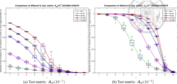
6.1 Similarity for different N. The size of test matrix is m = 2¹⁹, n = 2²⁰. For each cases, we repeat 30 times iSVD with integration method WY and plot out the box plot of similarity. The box plot represent the maximum, Q3, median, Q1, minimum for each inner product among 30 times. . . 43 6.2 Average iteration number to converge for different N and different size

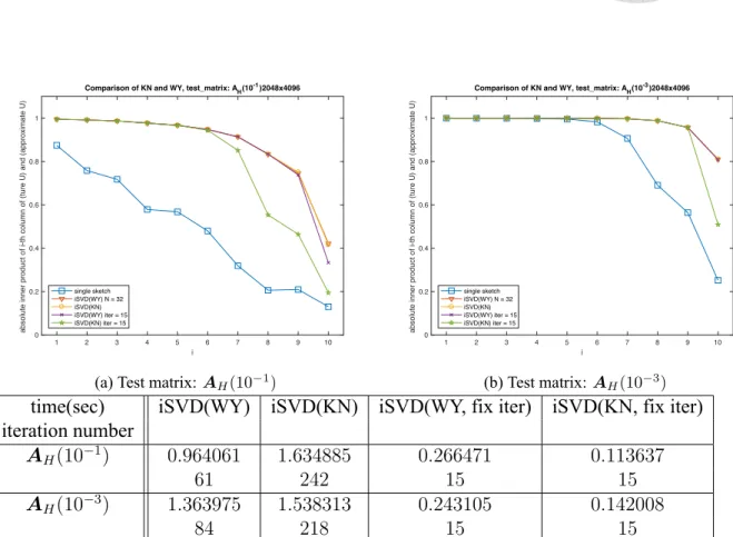
of test matrix. The size of test matrix is m = 2^d, n = 2^d+1 for d = 9, 11, 13, 15, 17, 19. Each point shows the average iteration number among 30 tests. . . 43 6.3 Comparison of the approximate singular vectors by using WY and KN.

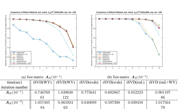
The size of test matrix is m = 2¹¹, n = 2¹² and the sampling number N = 32. All of these test use the same 32 sketched subspaces Q[i]. The first line in the legend represents the similarity of Q = Q_[1]. The second and third lines are the result from WY and KN respectively. The forth and fifth lines are from WY and KN respectively with fixed iteration number 15. . . 45 6.4 WY with different iteration numbers. The sketched subspaces Q_[i] are

same in Figure 6.3. The first line in the legend represents the similarity for the case Q = Q_[1]. The second line is the similarity from WY (with 61 iteration for AH(10⁻¹) and 84 iteration for AH(10⁻³) to converge).

The third to sixth lines are from WY with iteration number 5, 10, 15, 20 respectively. . . 46

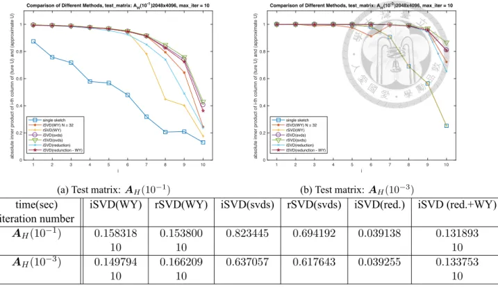
6.5 KN with different iteration numbers. The sketched subspaces Q_[i] are same in Figure 6.3. The first line in the legend represents the similarity for the case Q_[1]. The second line is the similarity from KN. The third to sixth lines are from KN with iteration number 5, 10, 15, 20 respectively. . 46 6.6 Similarity for WY with iSVD and rSVD, reduction, and svds. The number

of sketched subspaces in iSVD is N = 32. The number of sketching in rSVD is 32 ∗ 22, which is same as the total number of sketching in iSVD.

The algorithm red.+WY uses the result of reduction as the initial value of WY. . . 48 6.7 Similarity for the methods in 6.6 with the fixed iteration number 10 for WY. 49

xvi

doi:10.6342/NTU201702973

List of Tables

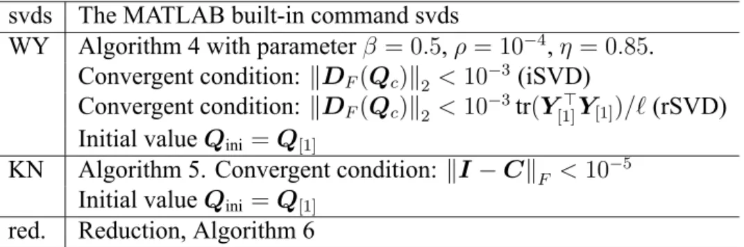
1.1 Notation in this thesis. . . 3 6.1 Abbreviation and detail information of the algorithm used in this section. 41

xviii

doi:10.6342/NTU201702973

Chapter 1 Introduction

Dimension reduction and feature extraction are important issues in data analysis, espe- cially for large scale data, to reduce the size or condense the information of analyzed data.

The goal is to reduce the time for further analysis or find out the key features in the data.

Singular value decomposition (SVD) is one of the technique to realize dimension reduc- tion. An SVD of an m × n matrix A takes the form A = UΣV^⊤, where U is an m × m orthogonal matrix, V is an n × n orthogonal matrix, and Σ is an m × n diagonal matrix with decreasing diagonal entries. In this representation, U, V are the left and right singu- lar vectors of A respectively. The diagonal entries of Σ are the singular vector of A. A rank-k approximation of A via SVD is given as

A = UkΣkV_k^⊤

where Uk, Vk are leading k singular vectors and Σk contains leading k singular values.

This low-rank approximation is called rank-k SVD of A. Rank-k SVD is the best rank-k approximation of A in the sense that it has the smallest 2-norm or Frobenius norm error.

Therefore, it is a good choice for dimension reduction in many cases.

Many algorithms are aimed at computing the SVD or rank-k SVD. However, these al- gorithms usually take at least O(m²n + mnk) for computing rank-k SVD of a real m× n (m ≤ n) matrix. Consequently, these algorithms cost lots of time to obtain the output re- sult. Some research [7, 10] proposed a method to randomly sketch the matrix into a smaller

subspace, and calculate approximate rank-k SVD in that space. This method is called ran- domized singular value decomposition (rSVD) in this thesis. The accuracy and precision of rSVD depend on the quality of random projection used to generate the subspace. How to increase the quality of random sketching and the accuracy of the approximation is an important issue in rSVD. In [4], integrated singular value decomposition (iSVD) is pro- posed to enhance the projected subspace and obtain a better result. The main idea of iSVD is using integration method to condense the information from multiple randomly sketching and output a better-sketched subspace.

In this thesis, some properties of iSVD and integration method will be studied. The concept of iSVD is introduced in Chapter 2. The key step of iSVD is the integration, which is a constraint optimization problem. In the Chapter 3, we show the integrated subspace defined previously is the only local maximizer of the constraint optimization problem.

The optimal solution and informal explanation of asymptotic behavior are introduced in the same chapter. These properties give the reason for using gradient type methods to solve this optimization problem. These methods are introduced and analyzed in Chapter 4. The similarity and difference between rSVD and iSVD with same sketching number are shown in the Chapter 5. The numerical experiment is shown in Chapter 6. Finally, the discussion and conclusion are given in Chapter 7.

The notations used in this thesis are as follows. The normal letters, such as a, α, denote the scalar. The bold lower case letters, such as a, α, denote the vector. The bold upper case letters, such as C, Γ, denote the matrix. Table 1.1 shows some frequently appeared notations in this thesis.

2

doi:10.6342/NTU201702973

A The matrix desired solving low-rank SVD.

m, n The number of rows and columns of A respectively. We assume m ≤ n.

k The given desired rank for low-rank approximation.

p The number of oversampling in rSVD and iSVD.

ℓ The total number of sampling in rSVD and iSVD for a single sketched subspaces.

ℓ = k + p. ℓ≪ m.

N The total number of sketched subspaces in iSVD.

⊗ The Kronecker product.

Ha,b The a × b commutation matrix.[9] For any a × b matrix M, vec(M^⊤) = Ha,bvec(M).

Qc The current iterator in the iterative method.

Q+ The iterator of next step in the iterative method.

Table 1.1: Notation in this thesis.

4

doi:10.6342/NTU201702973

Chapter 2

Overview of Integrated Singular Value Decomposition

Before introducing iSVD, we shall take a quick view of rSVD. The basic algorithm of rSVD from [7, 10] is stated as Algorithm 1. In this algorithm, SVD is only applied to an m× ℓ matrix and an ℓ × n matrix, which is much cheaper than applied on an m × n matrix if ℓ is small. The two main phases of rSVD are described in next two paragraphs.

Algorithm 1 Randomized SVD (rSVD)

Require: A (real m ×n matrix), k (number of desired rank for low-rank approximation), p (number of oversampling), ℓ = k + p (number of the sketched column),

Ensure: Approximate rank-k SVD of A ≈ !UkΣ!kV!_k^⊤

1: Generate a random matrix Ω

2: Assign Y ← AΩ

3: Compute Q whose columns are an orthonormal basis of Y

4: Compute the SVD of Q^⊤A = "WℓΣ!ℓV!_ℓ^⊤

5: Assign !Uℓ ← Q "Wℓ

6: Extract the largest k singular pairs from !Uℓ, !Σℓ, !Vℓto obtain !Uk, !Σk, !Vk

The first phase is randomly sketching a subspace of A. More precisely, compute the matrix Y = AΩ and find out the orthogonal basis of the range of Y as the approximate subspace Q. In this case, Ω is a randomly generated matrix. Both [7, 10] propose a commonly used Ω as Gaussian projection, which means the entries of Ω are independent identical standard normal distribution. This choice gives Y some structure of the column space from A and controls the error#

#QQ^⊤A− A##

2 < ϵ in high probability. Note that

QQ^⊤A is the approximate rank-ℓ SVD of A with the column space spanned by Y . The second phase is constructing an approximate rank-ℓ SVD QQ^⊤A. Only the SVD of Q^⊤A is needed to construct the SVD of the rank-ℓ matrix QQ^⊤A. Once the SVD of Q^⊤A = "WℓΣ!ℓV!_ℓ^⊤ is obtained, the SVD of QQ^⊤A can be computed as QQ^⊤A = (Q "Wℓ) !ΣℓV!_ℓ^⊤. Note that the column space of this approximation is already determined in the first phase. The purpose of this phase is revealing the singular values and singular vectors in correct arrangement, and then the leading k singular values and singular vectors can be extracted.

The technique of oversampling is proposed here. Suppose the desired rank is k, the number of sketches in the first phase can be chosen as ℓ = k + p for some positive integer p. The approximate rank-k SVD is obtained from rank-ℓ SVD by extracting the first k singular vectors and singular values.

Based on rSVD, iSVD uses multiple random sketched subspaces in the first phase of rSVD to gain more accurate result. The algorithm is stated as Algorithm 2. Three phases are included in this algorithm. The first phase is similar to the first phase of SVD. Instead of choosing only one random sketch in rSVD, iSVD choose multiple random sketches.

The second phase is integrating the subspaces obtained in the first phase and get an in- tegrated subspace Q. The third phase is same as the second phase of rSVD. They both construct the approximate rank-ℓ SVD.

Algorithm 2 Integrated SVD with multiple sketches (iSVD).

Require: A (real m × n matrix), k (desired rank of approximate SVD), p (oversampling parameter), ℓ = k + p (dimension of the sketched column space), q (exponent of the power method), N (number of random sketches)

Ensure: Approximate rank-k SVD of A ≈ !UkΣ!kV!_k^⊤

1: Generate n × ℓ random matrices Ω[i]for i = 1, . . . , N

2: Assign Y_[i] ← AΩ[i]for i = 1, ..., N

3: Compute Q_[i]whose columns are an orthonormal basis of Y_[i]

4: Integrate Q ← {Q[i]}^Ni=1

5: Compute the SVD of Q^⊤A = "WℓΣ!ℓV!_ℓ^⊤

6: Assign !Uℓ ← Q "Wℓ

7: Extract the largest k singular pairs from !Uℓ, !Σℓ, !Vℓto obtain !Uk, !Σk, !Vk

The key part of iSVD is how to define the integrated subspace in the second phase. The most intuitive idea is taking the arithmetic average of Q_[i] as Q, but the following state-

6

doi:10.6342/NTU201702973

ments show this is not a reasonable definition of the integrated subspace. The integrated subspace Q should represent the subspace integrated by Q_[i]. Each Q_[i] is an orthogonal matrix. Hence Q should also be an orthogonal matrix. However, the arithmetic average of Q[i]is not an orthogonal matrix. Therefore, the integrated subspaces should be defined by another form instead of the arithmetic average.

The integrated subspace in the second phase is defined by the following optimization

problem. ⎧

⎪⎪

⎪⎨

⎪⎪

⎪⎩

Q := argmin

Q

1 N

(N i=1

##Q[i]Q^⊤_[i]− QQ^⊤##²

F

subject to Q^⊤Q = Iℓ

(2.1)

The main idea of this definition is to define the integrated subspace that has the minimum summation of distances between each Q_[i] and Q, which is similar to the property of the arithmetic average in Euclidean space. Instead of the Euclidean distance between Q and each Q_[i], we use the distance between QQ^⊤and Q_[i]Q^⊤_[i]to preserve the invariant of right orthogonal transformation. Suppose Q_[1] = Q_[2]R for some orthogonal matrix R. Q_[1]

and Q[2] represent the same subspaces, so the measurement of error between Q[1], Q[i], and Q[2], Q[i] should be same. By using the relation

Q[1]Q^⊤_[1]− Q[i]Q^⊤_[i] = Q[1]RR^⊤Q^⊤_[1] − Q[i]Q^⊤_[i] = Q[2]Q^⊤_[2]− Q[i]Q^⊤_[i]

the error measured in (2.1) gives the same value, which means it preserved the invariant of right orthogonal transformation. However, it still needs some theoretical analysis to make sure whether this objective function is suitable for the integration step. Chapter 3 provides an informal explanation that the integrated subspace defined by 2.1 can capture the true singular vectors of the desired matrix A when N tends to be large.

8

doi:10.6342/NTU201702973

Chapter 3

Properties of Integrated Subspace

In this chapter, some properties of the integrated subspace defined in (2.1) are analyzed.

First, an equivalent maximization problem (3.1) is introduced. Next, we show the solu- tion of the optimization problem in (3.1) is the leading singular vectors of the arithmetic average of Q[i]Q^⊤_[i]. Then we provide an informal explanation for the asymptotic behavior of integrated subspace when N is large. Finally, we prove that the local maximizer of the optimization problem in (3.1) is unique up to a right orthogonal transform.

At the beginning, some equivalent problems should be introduced for the simplicity of analysis. The following theorem demonstrates an equivalent optimization problems of (2.1).

Theorem 3.0.1. The constraint optimization problem (2.1) is equivalent to the problem

⎧⎪

⎪⎨

⎪⎪

⎩

argmax

Q

1

2tr(Q^⊤P Q) Q^⊤Q = Iℓ

(3.1)

where P = _N¹ )N

i=1Q[i]Q^⊤_[i] is the arithmetic average of Q_[i]Q^⊤_[i]over all i.

Proof. From the relation between trace and Frobenius norm ∥M∥²_F = tr(M^⊤M ), the properties of trace tr(M₁M2) = tr(M2M1), and the orthogonality of Q and Q[i], the

Frobenius norm in the objective function of (2.1) can be rewritten as

##Q[i]Q^⊤_[i]− QQ^⊤##²

F = tr((Q[i]Q^⊤_[i]− QQ^⊤)^⊤(Q[i]Q^⊤_[i]− QQ^⊤))

= tr(QQ^⊤)− 2 tr(QQ^⊤Q[i]Q^⊤_[i]) + tr(Q[i]Q^⊤_[i])

= tr(Q^⊤Q)− 2 tr(Q^⊤Q_[i]Q^⊤_[i]Q) + tr(Q^⊤_[i]Q_[i])

= 2ℓ− 2 tr(Q^⊤Q[i]Q^⊤_[i]Q).

This equation leads to another representation of the objective function

1 N

(N i=1

##Q[i]Q^⊤_[i]− QQ^⊤##²

F = 2 ℓ

N − 21 N

(N i=1

tr(Q^⊤Q[i]Q^⊤_[i]Q) = 2 ℓ

N − 2 tr(Q^⊤P Q).

Since the constant does not affect the problem and the negative scalar changes minimize problem to maximize problem, (2.1) is equivalent to the problem

⎧⎪

⎪⎨

⎪⎪

⎩

argmax

Q

1

2tr(Q^⊤P Q) Q^⊤Q = Iℓ

which is the problem (3.1).

The optimization problem in the form (3.1) is more simple than the original form (2.1) for computing the derivative and further analyzing. So the simplified form (3.1) will be used in the following analysis.

3.1 Solution of the Optimization Problem

The solution of the maximize problem (3.1) is the integrated subspace we defined in (2.1).

Theorem 3.1.1 shows that the optimizer of this problem is consisted by the leading ℓ eigen- vectors of P .

Theorem 3.1.1 (Maximal Value of Objective Function). Let λ₁ ≥ λ² ≥ . . . ≥ λ^ℓ >

λℓ+1 ≥ . . . ≥ λm be the eigenvalues of P and let Q_∗ be the corresponding leading ℓ 10

doi:10.6342/NTU201702973

eigenvectors. Then the objective function in (3.1) has the upper bound

1

2tr(Q^⊤P Q)≤ 1 2

(ℓ i=1

λi

and the equality holds when Q = Q_∗R_∗for some ℓ × ℓ orthogonal matrix R∗.

Proof. The eigenvalue decomposition of P can be written as

P = Q_∗S_∗Q^⊤_∗ + Q_⊥S_⊥Q^⊤_⊥

where Q_⊥denote orthonormal basis of the space perpendicular to Q, S_∗ = diag(λ1, . . . , λℓ) and S_⊥ = diag(λ_ℓ+1, . . . , λ_m). Since Q_∗ and Q_⊥ spans the whole R^m, any orthogonal matrix Q can be represented as Q = Q_∗B + Q_⊥C with B^⊤B + C^⊤C = Iℓ. The objective function becomes

1

2tr(Q^⊤P Q)

= 1

2tr((Q_∗B + Q_⊥C)^⊤(Q_∗S_∗Q^⊤_∗ + Q_⊥S_⊥Q^⊤_⊥)(Q_∗B + Q_⊥C))

= 1

2tr(B^⊤S_∗B) + tr(C^⊤S_⊥C) by the relation Q^⊤Q_⊥ = 0

Let B = RST^⊤ be the SVD of B. By multiplying RT^⊤ from left and T R^⊤ from right to the both sides of the condition B^⊤B + C^⊤C = Iℓ, the new condition is given as RS²R^⊤+ RT^⊤C^⊤CT R^⊤ = RT^⊤T R^⊤ = Iℓ. By using this new condition and the inequality

tr((CT R)^⊤S_⊥CT R^⊤) =

m−ℓ

(

i=1

(ℓ j=1

λℓ+ic²_ij ≤

m(−ℓ i=1

(ℓ j=1

λjc²_ij = tr(S_∗RT^⊤C^⊤CT R^⊤)

where CT R^⊤= [cij], the upper bound of the objective function can be given as 1

2tr(Q^⊤P Q) = 1

2tr(B^⊤S_∗B) + tr(C^⊤S_⊥C)

= 1 2

*tr(T SR^⊤S_∗RST^⊤) + tr(C^⊤S_⊥CT R^⊤RT^⊤)+

= 1 2

*tr(S_∗RS²R^⊤) + tr(RT^⊤C^⊤S_⊥CT R^⊤)+

≤ 1

2tr(S_∗(RS²R^⊤+ RT^⊤C^⊤CT R^⊤)) = 1

2tr(S_∗) = 1 2

(ℓ i=1

λ_i.

The quality holds when)m−ℓ i=1

)ℓ

j=1λℓ+ic²_ij = )m−ℓ i=1

)ℓ

j=1λjc²_ij. This equation means CT R^⊤ = [cij] = 0, and hence C = 0. Therefore, Q = Q_∗R_∗ with B^⊤B = Iℓ and R_∗ = B.

Theorem 3.1.1 shows that the integrated subspace defined in (2.1) or (3.1) is actu- ally formed by the leading eigenvectors of the arithmetic average of Q[i]Q^⊤_[i]. The leading eigenvectors of P is same as the leading ℓ singular vectors of the matrix

,

Q[1]|Q[2]| · · · |Q[N ]

- . This form is used for explaining the similarity of rSVD and iSVD with same sketching number in Chapter 5.

3.2 Asymptotic Behavior of the Integrated Subspace

Now we give an informal explanation about the reason why the the integrated subspace defined in (2.1) or (3.1) can work in the iSVD algorithm. Please refer to [4] for more detailed statistical analysis.

To explain the reason, the following theorem in [4] should be introduced first.

Theorem 3.2.1. Let the SVD of A be A = UΣV^⊤ with distinct decreasing singular values. Let Q denote an orthogonal subspace spanned by Y = AΩ, where Ω is randomly generated by i.i.d. standard normal entries. Then

E.

Q_[i]Q^⊤_[i]/

= U ΛU^⊤

where Λ satisfies

12

doi:10.6342/NTU201702973

1. Λ is diagonal matrix

2. all diagonal entries are in the interval (0, 1)

3. the diagonal entries are decreasing if the singular values of A are distinct.

By the law of large number and Theorem 3.2.1, as the sample size N goes large, the arithmetic average P tends to a matrix with the same singular vectors of A in the cor- rect arrangement. Also, Theorem 3.1.1 shows that the optimizer defined in (3.1) is the leading singular vectors of P . Hence in the ideal case (N tends to infinity), iSVD can capture the leading singular vectors of A as Q and leads to an ideal result for the low-rank approximation.

3.3 Uniqueness of Local Maximizer

Recall that we focus on the problem in the form (3.1)

(+)

⎧⎪

⎨

⎪⎩ maxQ

1

2tr(Q^⊤P Q) Q^⊤Q = I_ℓ

.

Theorem 3.1.1 shows the optimal solution of the problem (+) is formed by the leading ℓ eigenvectors of the matrix P . However, this result dose not provide whether there exists another local maximum of this problem. The goal of the following derivation is Theo- rem 3.3.5, which shows that the only local maximum of the problem (+) is the orthogonal matrices that formed by the leading ℓ eigenvectors of P (up to right orthogonal trans- formation). The main idea of the following proof is checking the first and second order necessary condition for the nonlinear equality constraint optimization problem. More in- formation for the first and second order condition of optimization with equality constraint can be obtained in the book for introducing optimization problem. (For example, [6].)

We begin with checking the first order necessary condition of the problem (+).

Lemma 3.3.1 (First Order Necessary Condition). Suppose Q is a local maximizer of the problem (+) in the feasible set, i.e., the set collects all the m × ℓ orthogonal matrix. Then

Q satisfies the equation

(I − QQ^⊤)P Q = 0. (3.2)

and the corresponding Lagrange multiplier Λ ∈ R^ℓ×ℓ satisfies

Λ + Λ^⊤ = Q^⊤P Q. (3.3)

Proof. This equation is obtained from the first order condition for optimal solution of an equality constraint, which states that if x^∗ is a local maximizer of an equality constraint optimization problem, then the following equations hold

⎧⎪

⎨

⎪⎩

∇xL(x^∗, λ^∗) = 0

∇^λL(x^∗, λ^∗) = 0

where L is the Lagrangian of the equality constraint optimization problem and λ^∗ is the corresponding Lagrange multiplier.

Notice that any m × n matrix M can be seen as an mn vector by vectorizing M as vec(M). Also, one of the relation between vec(•) and Kronecker product ⊗ is vec(AXB) = (B^⊤⊗ A) vec(X). By using these technique, the Lagrangian of (+) is given as

L(Q, Λ) = 1

2tr(Q^⊤P Q)− tr(Λ^⊤(Q^⊤Q− I^ℓ))

= 1

2vec(Q)^⊤vec(P Q) − vec(Λ)^⊤vec(Q^⊤Q− Iℓ)

= 1

2vec(Q)^⊤(Iℓ⊗ P ) vec(Q) − vec(Λ)^⊤vec(Q^⊤Q− I^ℓ) and the first order conditions can be represented by the derivative of Lagrangian as

⎧⎪

⎨

⎪⎩

∇vec(Q)L(Q, Λ) = (I ⊗ P ) vec(Q) − [K^ℓ,m(Q⊗ I^ℓ) + (Iℓ⊗ Q)] vec(Λ) = 0

∇vec(Λ)L(Q, Λ) = vec(Q^⊤Q− Iℓ) = 0

where K_ℓ,mdenotes the communication matrix corresponding to ℓ×m matrix. By folding 14

doi:10.6342/NTU201702973

the vectorized matrix back, the above equations leads to

⎧⎪

⎨

⎪⎩

P Q− Q(Λ + Λ^⊤) = 0 Q^⊤Q− I^ℓ = 0.

Applying Q^⊤to the left of each side in the first equation and Using the second equation derives the relation Λ + Λ^⊤= Q^⊤P Q. By substituting (Λ + Λ^⊤) as Q^⊤P Q in the first equation, the first order conditions can be rewritten as

⎧⎪

⎨

⎪⎩

(I− QQ^⊤)P Q = 0 Q^⊤Q = Iℓ

Lemma 3.3 gives the necessary conditions for feasible points and the corresponding Lagrange multiplier. The following lemma improves the result. It provides the explicit solutions that satisfy these conditions.

Lemma 3.3.2. Let Q be a feasible points of the problem (+). Then Q satisfies the first

order condition (3.2) if and only if each column of QR is an eigenvector of P for some orthogonal matrix R ∈ R^ℓ×ℓ.

Proof. For the ‘if’ part, since the columns of QR are eigenvectors of P , the connection between P and QR is given as P QR = QRS, where S is a diagonal matrix with the corresponding eigenvalues on its diagonal entries. By directly calculation,

(I− QQ^⊤)P QR = (I− QQ^⊤)QRS = 0

and hence

(I− QQ^⊤)P Q = 0

by multiplying R^⊤to the right of both sides. This equation shows that Q satisfies the first order condition (3.2).

For the ‘only if’ part, suppose Q satisfies the first order condition (I − QQ^⊤)P Q = 0. Since (I − QQ^⊤) is the projection matrix onto the orthogonal complement of the range of Q, the first order condition means that the component of each columns of P Q in the orthogonal complement is 0, i.e., each column of P Q is a vector in the range of Q.

Therefore, each column of P Q can be written as the linear combination of the columns of Q and hence

P Q = QB

for some B ∈ R^ℓ×ℓ. By applying Q^⊤ to the left of both sides, the equation becomes B = Q^⊤P Q which is a symmetric matrix. Therefore, B has eigenvalue decomposition B = RSR^⊤for some orthogonal matrix R and diagonal matrix S. This decomposition gives the relation

P Q = QRSR^⊤ and hence

P (QR) = (QR)S

by multiplying R to the right of both sides. This equation shows each column of (QR) is an eigenvector of P since S is diagonal.

Now we check the second order condition. The preparation for computing second order condition is finding the null space spanned by the gradient of constrains. Let g(Q) denote the constraint function g(Q) = vec(Q^⊤Q− Iℓ) = 0, and NQ denote the null space of the linear space spanned by the gradients of constrains ∇vec(Q)g(Q) at Q. The following lemma gives some explicit representations of the null space N^Q.

Lemma 3.3.3. The null space N^Q is given as NQ =0

vec(Z) : Z ∈ R^m×ℓ, Q^⊤Z + Z^⊤Q = 01

or equivalently,

NQ =0

vec(QB + Q_⊥C) : B ∈ R^ℓ×ℓ, C ∈ R^{(m−ℓ)×ℓ}, B =−B^⊤1 16

doi:10.6342/NTU201702973

where Q_⊥is a m × (m − ℓ) orthogonal matrix satisfies Q^⊤_⊥Q = 0, i.e., Q_⊥contains the basis of orthogonal complements of the range of Q.

Proof. By direct calculation, the gradient matrix of constraints at Q is given as

∇vec(Q)g(Q) = Kℓ,m(Q⊗ I^ℓ) + (Iℓ⊗ Q).

According to the definition of NQ, every element vec(Z) in NQ satisfies the condition

[K_ℓ,m(Q⊗ Iℓ) + (I_ℓ⊗ Q)]^⊤vec(Z) = 0

which leads to

Q^⊤Z + Z^⊤Q = 0.

This computation shows that NQ ⊂ 0

vec(Z) : Z ∈ R^m×ℓ, Q^⊤Z + Z^⊤Q = 01 . The equality can be proved by computing the dimension of each space.

Since the columns of Q and Q_⊥ can span R^m, any matrix Z ∈ R^m×ℓ can be repre- sented as Z = QB + Q_⊥C, where B ∈ R^ℓ×ℓ and C ∈ R^{(m−ℓ)×ℓ}. Another equivalent condition for null space is obtained by plugging this representation into the condition

Q^⊤(QB + Q_⊥C) + (QB + Q_⊥C)^⊤Q = B + B^⊤ = 0.

Hence

NQ =0

vec(QB + Q_⊥C) : B ∈ R^ℓ×ℓ, C ∈ R^{(m−ℓ)×ℓ}, B =−B^⊤1 .

The second order necessary condition can be written out by the explicit form of the null space.

Lemma 3.3.4 (Second Order Necessary Condition). Suppose Q is a local maximizer of

(+). Then Q satisfies the inequality

tr(Z^⊤P Z− Z^⊤ZQ^⊤P Q)≤ 0.

for all vec(Z) ∈ NQ.

Proof. The second order necessary condition is

vec(Z)^⊤∇²QQL(Q, Λ) vec(Z) ≤ 0

for all vec(Z) ∈ NQ. By the relation of Lagrange multiplier at the feasible point (3.3) as Λ + Λ^⊤ = Q^⊤P Q, the gradient ofL by Q can be written as

∇QL(Q, Λ) = (I ⊗ P ) vec(Q) − [Kℓ,m(Q⊗ Iℓ) + (I_ℓ⊗ Q)] vec(Λ)

= (I⊗ P ) vec(Q) − vec(QΛ^⊤+ QΛ)

= (I⊗ P ) vec(Q) −.

(Λ^⊤+ Λ)⊗ I^m/

vec(Q)

= (I⊗ P ) vec(Q) − (Q^⊤P Q⊗ Im) vec(Q) Hence the Hessian matrix is

∇²QQL(Q, Λ) = I ⊗ P − Q^⊤P Q⊗ Im

The second order necessary condition can be rewritten as

vec(Z)^⊤∇²QQL(Q, Λ) vec(Z) = vec(Z)^⊤vec(P Z − ZQ^⊤P Q)

= tr(Z^⊤P Z− Z^⊤ZQ^⊤P Q)≤ 0.

Finally, the main theorem of this part can be proved by the first and second order necessary conditions.

Theorem 3.3.5 (Local Maximizer of Optimization Problem). Let λ₁ ≥ λ² ≥ . . . ≥ λ^ℓ >

λℓ+1 ≥ . . . ≥ λm be the eigenvalues of P and let Q_∗ be the corresponding leading ℓ 18

doi:10.6342/NTU201702973

eigenvectors. Then Q is an local maximizer of (+) if and only if Q = Q_∗R_∗ for some ℓ× ℓ orthogonal matrix R∗.

Proof. By Lemma 3.3.2, for all Q that satisfies the first order condition, there exists an orthogonal matrix R such that each column of QR is an eigenvector of P . By computing eigenvalue value decomposition,

P = (QR)S(QR)^⊤+ Q_⊥S_⊥Q^⊤_⊥

where Q_⊥contains (m − ℓ) eigenvector that orthogonal to QR, S = diag(s1, s2, . . . , sℓ), S_⊥ = diag(s^⊥₁, s^⊥₂, . . . , s^⊥_m−ℓ) and s₁, s₂, . . . , s_ℓ, s^⊥₁, s^⊥₂, . . . , s^⊥_m−ℓform all eigenvalues of P . By Lemma 3.3.3, the element ⃗(Z) ∈ N^Q can be represented as Z = QB + Q_⊥C with B = −B. These relations lead to a representation of second order condition as

tr(Z^⊤P Z− Z^⊤ZQ^⊤P Q)

= tr((QB + Q_⊥C)^⊤((QR)S(QR)^⊤+ Q_⊥S_⊥Q^⊤_⊥)(QB + Q_⊥C)

− (QB + Q⊥C)^⊤(QB + Q_⊥C)Q^⊤((QR)S(QR)^⊤+ Q_⊥S_⊥Q^⊤_⊥)Q)

= tr(B^⊤RSR^⊤B) + tr(C^⊤S_⊥C)− tr(B^⊤BRSR^⊤)− tr(C^⊤CRSR^⊤)≤ 0

By the properties of trace and the relation B = −B^⊤, tr(B^⊤BRSR^⊤) = tr(BRSR^⊤B^⊤) = tr(B^⊤RSR^⊤B). Also, since RR^⊤ = Iℓ, tr(C^⊤S_⊥C) = tr(RR^⊤C^⊤S_⊥C) = tr((CR)^⊤S_⊥(CR) Hence the second order condition in Lemma 3.3.4 can be written as

tr(B^⊤RSR^⊤B) + tr(C^⊤S_⊥C)− tr(B^⊤BRSR^⊤)− tr(C^⊤CRSR^⊤)

= tr((CR)^⊤S_⊥CR)− tr((CR)^⊤(CR)S_⊥)

=

(m−ℓ)(

i=1

(ℓ j=1

s^⊥_i c²_ij −

(m−ℓ)(

i=1

(ℓ j=1

sjc²_ij ≤ 0

for all CR = [c_ij]∈ R^m×(m−ℓ).

Let Q_∗ denotes the leading ℓ eigenvectors of P . Suppose QR contains eigenvector other than leading ℓ singular vectors of P . Then s^⊥_a > sbfor some a and b. Now pick [c_ij]

as c_ab= 1 and cij = 0 otherwise. Then

(m(−ℓ) i=1

(ℓ j=1

s^⊥_i c²_ij−

(m(−ℓ) i=1

(ℓ j=1

sjc²_ij = s^⊥_a − s^b > 0.

This inequality conflicts to the second order necessary condition. On the other hand, sup- pose QR = Q_∗. Then S = diag(λ₁, λ2, . . . , λℓ) and S_⊥ = diag(λℓ+1, . . . , λm). Hence for all [c_ij]∈ R^m×(m−ℓ).

(m(−ℓ) i=1

(ℓ j=1

s^⊥_i c²_ij −

(m(−ℓ) i=1

(ℓ j=1

sjc²_ij ≤ (λ^ℓ+1− λ^ℓ)

(m(−ℓ) i=1

(ℓ j=1

sjc²_ij ≤ 0

by (λ_ℓ+1 − λ^ℓ) < 0 and)_(m−ℓ)

i=1

)ℓ

j=1sjc²_ij ≤ 0. This inequality obeys the second order necessary condition.

To sum up, a feasible point Q satisfies the first and second order necessary condition if and only if Q = Q_∗R_∗ for some orthogonal matrix R_∗ = R^⊤. Lemma 3.1.1 shows that Q_∗R_∗ is global maximizer, and hence local maximizer.

Theorem 3.3.5 provides that the only type of local maximizer is the orthogonal matrix that formed by the leading ℓ eigenvectors of the matrix P (with some right orthogonal transformation), which is the integrated subspaces defined in (2.1) or (3.1). This result shows that if a line search can prevent the iterator from saddle points, it can find out the integrated subspace successfully.

20

doi:10.6342/NTU201702973

Chapter 4

Integration Method

As shown in Chapter 2, the integrated subspace is the leading eigenvectors of the ma- trix P , or the singular vectors of the matrix

,

Q_[1]|Q[2]| · · · |Q[N ]

-

.. Therefore, canonical SVD (for example, the SVD routine in MATLAB or LAPACK [2]) can be applied to solve this eigenvectors problem. However, the computational complexity of canonical SVD is O(N²mℓ²), which is much slower when N increasing. Hence in this chapter, we intro- duce some other methods to compute the integrated subspace with different computational complexity than O(N²mℓ²).

4.1 Line Search Type Method

Since the integrated subspace is defined by an optimization problem, it is reasonable to use the algorithm for solving the optimization problem for computing the integrated subspace.

A classical method for solving the optimization problem is line search methods. Gradient descent method (in our case, gradient ascent method) is widely used among the line search methods. The update scheme for unconstraint gradient ascent method is

x_k+1 = x_k+ τ_k∇f(xk)

where f is the objective function and τ_k is the step size needed to search in the n-th it- eration. In the viewpoint of line search, in each iteration, we define a curve γ_k(τ ) =

xk+ τk∇f(xk). This curve is a straight line stating at the point xkand point to the direc- tion ∇f(xk), which is the steeps ascent direction of objective function at x. The point for next iteration is given by finding a suitable step size τ and define xk+1 = γk(τ ). These explanations shows the main concept of gradient ascent method. It tries to find the optimal solution by walking along the curve with steepest direction in each step with suitable step size.

The main issue for this algorithm is to find a suitable step size τ. If the step size is too large, it may be difficult to reach the optimal solution because it may walk too far.

However, if the step size is too small, it may need more iteration to reach the optimal solution. One of the popular methods for selecting step size is using the back tracking method with Armijo-Wolfe condition (for maximization problem)

f (x_k+ τ_kp_k)≥ f(xk) + ρτ_kp^⊤_k∇f(xk) p^⊤_k∇f(xk+ τkpk)≤ ρ2p^⊤_k∇f(xk)

where ρ, ρ2 is parameters that can be chosen and pk = ∇f(x^k) in gradient ascend. The second condition always holds due to the design of algorithm. Hence we just need to focus on the first condition. We use Armijo rule for simplicity in the following content.

The back tracking method tries to find the step size τ_k satisfied the Armijo rule by the following steps. First, assign an initial guess of step size, such as 1. Then test whether this step size satisfies the Armijo rule. Suppose not, multiply this step size by a positive constant β < 1 and test it again. Repeat these processes until the step size satisfies the Armijo rule and set it into τk.

For the constraint optimization problem, the gradient ascent method needs to be mod- ified. Here we choose to use the viewpoint of the gradient ascent method on Stiefel man- ifold. The Stiefel manifold is the manifold consisted of all m × ℓ orthogonal matrices

S^m,ℓ =0

Q∈ R^m×ℓ: Q^⊤Q = I1

which is exactly our constraint in the optimization problem.

22

doi:10.6342/NTU201702973

Define

F (Q) = 1

2tr(Q^⊤P Q) as our objective function. We denote the gradient of F at Q as

GF(Q) = P Q

where the equality can be computed easily. On the manifold, the gradient in the Euclidean space may not represent the direction (tangent) at a point. Hence we need to project the gradient to the tangent space on the manifold for further derivation.

Lemma 4.1.1. The projected gradient of F onto the tangent space T^QS^m,ℓof Stiefel man- ifold S^m,ℓis

DF(Q) = (I− QQ^⊤)P Q.

Proof. First we find a necessary and sufficient condition for X being in TQSm,ℓ. For all X ∈ TQSm,ℓ, find a path Γ(t) in Sm,ℓwith Γ(0) = Q and Γ^′(0) = X. From Γ(t)^⊤Γ(t) = I, differentiate each side by t and take t = 0, we have

X^⊤Q + Q^⊤X = 0, (4.1)

which gives a necessary condition for X ∈ TQSm,ℓ. There are ℓ(ℓ + 1)/2 conditions for X in (4.1) and the dimension ofT^QS^m,ℓ is mℓ − ℓ(ℓ + 1)/2, which means (4.1) is also a sufficient condition for X ∈ T^QS^m,ℓ. By taking vec to each sides of (4.1), we get the equality

[(Q^⊤⊗ Iℓ)Km,ℓ+ (Iℓ⊗ Q^⊤)] vec(X) = 0.

Define T = K_ℓ,m(Q⊗ Iℓ) + (I_ℓ⊗ Q) and get T^⊤vec(X) = 0. This shows that the tangent space (after vectorizing each elements) is contained in the null space of T^⊤. One can compute the rank of T and shows that the null space of T^⊤ is actually the tangent space. Hence the projection matrix onto the tangent space is given by (I − PT), where PT = T (T^⊤T )⁺T^⊤and (T^⊤T )⁺denoted the Moore-Penrose pseudo-inverse. With P_T,

DF can be given via vec(D_F) = (I − PT) vec(GF). With some calculation, we have T = (I_ℓ⊗ Q)(Iℓ² + K_ℓ,ℓ) and thus

T^⊤T = (Iℓ² + Kℓ,ℓ)^⊤(Iℓ⊗ Q)^⊤(Iℓ⊗ Q)(Iℓ² + Kℓ,ℓ)

= (I_ℓ² + Kℓ,ℓ)(I_ℓ² + Kℓ,ℓ) = 2(I_ℓ² + Kℓ,ℓ).

Then the projection matrix P_T can be calculated as:

PT = T (T^⊤T )⁺T^⊤

= (Iℓ⊗ Q)(Iℓ² + Kℓ,ℓ)1

2(Iℓ² + Kℓ,ℓ)⁺(Iℓ² + Kℓ,ℓ)^⊤(Iℓ⊗ Q)^⊤

= 1

2(Iℓ⊗ Q)(Iℓ² + Kℓ,ℓ)(Iℓ⊗ Q^⊤)1

2(Iℓ⊗ QQ^⊤) + 1

2(Q^⊤⊗ Q)K^m,ℓ. Hence, by vec(DF) = (I − P^T) vec(GF),

vec(D_F) = (Iℓ² −1

2(Iℓ⊗ QQ^⊤)− 1

2(Q^⊤⊗ Q)K^m,ℓ) vec(GF)

= vec(G_F)− 1

2(I_ℓ⊗ QQ^⊤) vec(G_F)− 1

2(Q^⊤⊗ Q)Km,ℓvec(G_F)

= vec(GF)− 1

2vec(QQ^⊤GF)−1

2vec(QG^⊤_FQ) and D_F can be written as

DF = 2

I− 1 2QQ^⊤

3

GF −1

2QG^⊤_FQ. (4.2)

Since we have the property Q^⊤GF(Q) = GF(Q)^⊤Q here, we can get DF(Q) = (I− QQ^⊤)GF(Q). This completes the proof.

Algorithm 3 is rewritten from [1] by the notation in this thesis and the projected gra- dient as above. Note that the function F (M) denote the function that orthogonalize M first (hence this point is in the Stiefel manifold) and then plug into F .

The basic concept of Algorithm 3 is same as the gradient ascent method described previously. For each step, we find the projected gradient, which is the steepest direction on the manifold. Then we walk along this direction with a suitable step size decide by backtracking and Armijo-Wolfe condition. The difference is that we need to retract back

24

doi:10.6342/NTU201702973

Algorithm 3 Integration of {Q[i]}^Ni=1based on Armijo line search.

Require: Q_[1], Q[2], . . . , Q[N ](subspace matrices), Qini(initial guess), τ₀ > 0 (initial step size), β ∈ (0, 1) (scaling parameter for step size searching), ρ ∈ (0, 1) (parameters for step size searching)

Ensure: Integrated subspace matrix Q based on Armijo line search

1: Initialize the current iterate Q_c ← Qⁱⁿⁱ

2: while (not convergent) do

3: Compute the gradient on manifold X = (I_m− QcQ^⊤_c)P Qc

4: Find the smallest integer j ≥ 0 such that the following inequality holds:

F (Qc+ τ0β^jX)≥ F (Q^c) + τ0β^jρ∥X∥²F

5: Orthogonalize (Q_c+ τ0β^jX) (for example, by QR-decomposition or polar decom- position) as Q₊

6: Assign Qc ← Q⁺

7: end while

8: Output Q = Q_c

to the manifold before we calculate the objective function and before the next iteration. In this algorithm, it uses orthogonalization as the retraction.

In [1], the convergent theorem is also provided. Here we translate the theorem and write down the most important part as Theorem 4.1.2. Note that in the theorem, a critical point x_∗ (the points that make projected gradient is 0) is stable, if for any neighborhood U around x_∗, there exists another neighborhood V around x∗, such that if the initial value start in V, then after any finite steps, the result will be in U. A critical point is asymptotically stable if it is stable, and the condition also holds as the number of steps tends to infinity.

A critical point is unstable if it is not stable.

Theorem 4.1.2 (Convergence theory for Algorithm 3). Let λ₁ ≥ λ2 ≥ . . . ≥ λℓ >

λℓ+1 ≥ . . . ≥ λm be the eigenvalues of P and let Q_∗ be the corresponding leading ℓ eigenvectors. Algorithm 3 converge to the orthogonal matrix Q with each column are eigenvectors of P . Among all the critical points, Q_∗(up to a right orthogonal transform) is the only asymptotically stable point with the linear convergent rate. Other critical points are unstable.

This theorem gives the promise of the convergence. Also, our result for the property of optimization problem in Chapter 3 can support this result. The critical points are actually the points satisfying first order condition 3.2. Among these points, only Q_∗ satisfies the

second order condition, which is related to the condition of stable points.

However, same as the traditional gradient ascent method, the convergent rate of the Algorithm 3 is linear. This could be a problem since it might take many steps to converge.

Here we provide another algorithm. Algorithm 4 is rewritten by the notation and objective function in this thesis from the algorithm proposed by Wen and Yin [11].

This algorithm is based on gradient ascent method which is similar to Algorithm 3.

However, some modification is introduced for this algorithm. The method to retract the point back to the manifold is changed in this modified algorithm. The searching path at current point Q_c is defined as Γ_Qc(τ ) = (I − ^τ₂M )⁻¹(I + ^τ₂M )Qc, where M = GQ^⊤_c − QcG^⊤ and G = P Q_c is the gradient of the objective function in Euclidean space. By using Woodbury matrix identity, the searching path is same as

ΓQc(τ ) = Qc− τL(I^2ℓ+1

2τ R^⊤L)⁻¹R^⊤Qc (4.3) where L = [−G Qc] and R = [Qc G]. This modification decreases the matrix size to compute inverse. As mentioned in [11], this path also satisfies some properties, hence Theorem 4.1.2 also holds for this algorithm.

Algorithm 4 also uses the Barzilai-Borwein step size [3] (BB step size) to accelerate this gradient method, and the nonmonotone strategy in [12] to prevent stuck in the local optimal points. The Armijo rule in the Algorithm 4 is

F (Γ_Qc(τ ))≥ F (ΓQc(0)) + τ σ dF (Γ_Qc(t)) dt

44 44

t=0

.

The nonmonotone strategy in [12] modified the Armijo rule by

F (ΓQc(τ ))≥ c + τσ dF (Γ_Qc(τ )) dt

44 44

t=0

where c is a scalar updated in each iteration by c ← (ηζc + F ((Q⁺))/(ηζ + 1) and then ζ ← ηζ + 1 for a given parameter η. The initial value of c is F (Qⁱⁿⁱ). This condition soften the Armijo rule and increase the chance to jump out the local minimum.

26

doi:10.6342/NTU201702973