基於彩色深度攝影機及慣性感應器之自我運動估測

(1)

國立臺灣大學電機資訊學院資訊網路與多媒體研究所碩士論文

Graduate Institute of Networking and Multimedia College of Electrical Engineering and Computer Science

National Taiwan University Master Thesis

基於彩色深度攝影機及慣性感應器之自我運動估測 Ego-motion Estimation Based on RGB-D Camera and Inertial

Sensor

鄂彥齊 Yen-Chi E

指導教授：洪一平博士 Advisor: Yi-Ping Hung, Ph.D.

中華民國 104 年 7 月

July, 2015

(2)

(3)

致謝

在碩班兩年的期間內，感謝洪一平教授所給予的指導與提點，讓我研究上能有所斬獲。洪老師總是願意點出我在研究上的不足，並且不吝給我建議，讓我得以改善研究上的問題，並從中學習到研究方法。

在論文研究的過程中，感謝冠文學長平時的教導以及幫助，經由學長的提點讓我學習到如何去化解在實作上所遇到的困難。同時也感謝欣叡學長總是很有熱忱地與我討論 IMU 的相關知識，讓我學習到不少。

除此之外，很感謝沈超，柏彰，歆如，冠翔以及其他實驗室同學在研究路途上的陪伴與鼓勵，與你們共度這兩年讓我能有所成長，也感謝實驗室裡許多碩、博班的學長姊以及學弟妹的陪伴。最後要感謝我的父母及家人在我就學期間所給予的支持與鼓勵。

(4)

中文要

自我運動估測在機器人控制及自動化上有相當廣泛的應用。正確的區域自我運動估測可以幫助機器人了解、感知周遭環境，並建構出走過的路徑。在這篇論文裡，我們提出了一個結合基於關鍵影格的視覺里程計及慣性資料的自我運動估測系統。系統硬體包括擷取影像的彩色深度攝影機和取得慣性資料的慣性測量單元。

兩張連續影像間的攝影機運動經由視覺特徵的對應關係來進行計算。剛體限制可以有效地將初始對應點裡的異常對應點去除。此外，

我們估測運動的過程中利用隨機抽樣一致性算法來處理剩餘異常對應點的影響。這些方式都能讓我們確保在進行攝影機運動估算時所用的對應點幾乎都是正確的對應。

我們進行了各種實驗來證明演算法的穩固性和正確性，以及正確地處理真實場景的能力。

關鍵字：自我運動、運動估測、視覺里程計、彩色深度攝影機、慣性測量單元

(5)

Abstract

Ego-motion estimation has a wide variety of applications in robot control and automation. Proper local estimation of ego-motion benefits to recognize surrounding environment and recover the trajectory traversed for autonomous robot. In this thesis, we present a system that estimates ego-motion by fusing key frame based visual odometry and inertial measurements. The hardware of the system includes a RGB-D camera for capturing color and depth images and an Inertial Measurement Unit (IMU) for acquiring inertial measurements.

Motion of camera between two consecutive images is estimated by finding correspondences of visual features. Rigidity constraints are used to efficiently remove outliers from a set of initial correspondence. Moreover, we apply random sample consensus (RANSAC) to handle the effect of the remaining outliers in the motion estimation step. These strategies are reasonable to in- sure that the remaining correspondences which involved in motion estimation almost contain inliers.

Several experiments with different kind of camera movements are performed to show that the robustness and accuracy of the ego-motion estimation algorithm, and the ability of our system to handle the real scene data correctly.

Key words:ego-motion, motion estimation, visual odometry, RGB-D camera, inertial measurement unit

(6)

List of Figures

1.1 ego-motion applications . . . 2

2.1 Kneip et al’s method combing monocular camera and IMU . . . 5

2.2 The perception hand-held device . . . 5

2.3 Overall scheme of Hirschmuller et al.’s method . . . 6

3.1 system overview . . . 8

3.2 When the current frame is at time t, then the motion between t and t-1, t and t-2, ... , t and 1 will be computed and select the best one from all results. 9 3.3 Feature Based Visual Odometry with Spatial Constraints . . . 10

3.4 Consideration of Feature Matching . . . 10

3.5 An example of finding feature correspondence. . . 11

3.6 An example of correspondences between 2-D matching (left) and 3-D point clouds (right). Every green line means a corresponding pair. . . 12

3.7 An example of correspondences between 2-D matching (left) and 3-D point clouds (right). Every red line means a incorrect corresponding pair ( i.e. outlier ). . . 12

3.8 The relative distance between P_iand P_kshould be the same at time t and t− 1 ( i.e. the length of orange line keeps unchanged ). Similarly, the gray line also keeps unchanged. . . 14

(9)

3.9 A vector ⃗a = P_i^t⁻¹− Pkt−1is formed by two 3-D points P_i^t⁻¹ and P_k^t⁻¹ at time t− 1. This vector becomes vector ⃗b = Pit− Pkt by suffering a transformation at time t (left). The rotation angle constraint is setting a

limitation of the angle θ between vector ⃗a and ⃗b (right). . . . 15

3.10 An example of the consistent table. . . 16

3.11 A 5× 5 example to show how to finding the consistent subset. . . 17

3.12 feature matching results . . . 18

3.13 Motion Estimation Scenario . . . 18

3.14 For computing the motion of F_n, we calculate the motion to F_n from KF₁ KF₅. Then, selecting the motion with minimal overall motion error and replacing the key frame with highest overall motion error. . . 21

4.1 The ego-motion estimation device . . . 23

4.2 Two scenes of the testing rooms . . . 23

4.3 The number of initial correspondences, consistent correspondences and remaining inliers after RANSAC between two images. . . 24

4.4 Estimated result with translatory motion only . . . 24

4.5 Estimated results of a turn round trip . . . 26 4.6 Estimated results of long-term round trip. The red trajectory is the visual

alone result, the blue trajectory is the fusion result and the green trajectory is the ground truth. The total distance of blue and red path are 142.9 m and 116.3 m, respectively. The manually measured ground truth is 119.7 m. 27

(10)

List of Tables

4.1 Evaluation of Translation Test . . . 25 4.2 Comparison with other methods . . . 27

(11)

Chapter 1 Introduction

1.1 Ego-motion Estimation

Environment perception plays an important role on robotics system for autonomously navigation because surrounding environment understanding can help robot avoid colli- sions and reach the target position correctly. With an accurate estimate of the robot current state is good for autonomous navigation and Simultaneous Localization And Mapping (SLAM) [1].

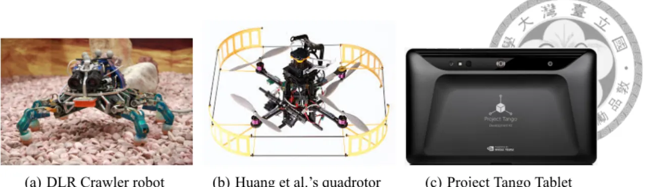
Stelzer et al. in the German Aerospace Center (DLR) produce a six-legged walking robot, attached with stereo cameras and inertial sensors for motion estimation. Accord- ing to the estimated motion, the robot can be navigated to walk in unknown terrain. A.

S. Huang et al. propose a quadrotor carries RGB-D cameras and laser scanner for state estimation and then control quadrotor’s flight. Google Project Tango applied ego-motion estimation on the mobile devices (e.g. tablet or smart phone) for positioning. Obviously, ego-motion estimation becomes more and more important issue for robotics tasks such as robot navigation, drone control and mobile device positioning.

(12)

(a) DLR Crawler robot (b) Huang et al.’s quadrotor (c) Project Tango Tablet

Figure 1.1: ego-motion applications

Visual odometry, which determine camera motion according to the associated camera images, gives accurate estimation of translatory movement, but it is possibly inaccurate to estimate the rotational movement. In contrast, the Inertial Measurement Unit, which determine camera motion by integrating the measurements from accelerometers, gyroscopes and magnetometers, provides accurate orientation estimation, but produces drift in long- term translation estimation due to the integration noise. Therefore, combining visual and inertial measurements has complementary properties which make a more robust motion estimation for many robotic applications.

This thesis describes a system that estimates camera motion of an agent, which moves unconstraint in the static scene by attached RGB-D camera and inertial sensor. Our expec- tation is to integrate vision and inertial data incrementally to estimate the camera motion with respect the starting position and recover the trajectory.

1.2 Hardware Sensors

RGB-D cameras are sensing systems that capture RGB images along with per-pixel depth information. In our work, we use Microsoft Kinect, which captures 640 x 480 reg- istered image and depth pixels. Kinect analyses a speckle pattern of infrared laser light to sensing the depth informtaion and its cameras allow the capture of reasonably accurate depth and color information at high data rates of up to 30 fps.

Inertial Measurement Unit (IMU) contains a number of micro-electrical-mechanical (MEMS) sensors including gyroscope, accelerometer, and magnetometer. The information from each of these sensors is combined through the sensor fusion process to determine

(13)

the motion of the IMU in real world. In our work, the Oculus Rift, which acquires iner- tial data at about 50 Hz is used as the inertial sensor to integrate measurements from accelerometer, gyroscope and magnetometer to derive the orientation.

1.3 Organization of the Thesis

The remainder of this thesis is structured as follows. In Section 2, we provide an overview of the related works. Section 3 introduces the theoretical detail of our algorithm, computing ego-motion based on feature correspondences and fusing with inertial data for robust motion estimation. Section 4 describes the experimental setup of our system, then presents extensive results on different evaluation schemes. In Section 5 we conclude this thesis and discuss some future works about this work.

(14)

Chapter 2 Related work

Ego-motion estimation has been developed for a long time and become more and more popular in many robotics applications. A complete tutorial of visual odometry has been given by Scaramuzza et al. [2] at ETH.

The term visual odometry was coined in 2004 by Nister et al. [3]. In the past few years, several ego-motion estimation methods have been developed by using different sensors such as Kneip et al. [4] combine monocular camera and IMU, Geiger et al. [5]

use stereo cameras and Hirschmuller et al. [6] perform a system combing stereo cameras and IMU. In this section, we will give an overview of some related work about visual odometry.

2.1 Single Camera and IMU

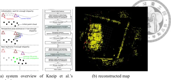
Kneip et al. proposed a robust, continuous pose computation method combing single camera and IMU [4]. Firstly, a local point cloud is iniitalized from two frames with sufficient disparity. If the disparity between current frame and previous key frame is not large enough, then the relative camera pose will be determined using the pre-generated point cloud. In contrast, if the disparity is large enough, then current frame and key frame are used to triangulate the new point cloud and the current will be treated as key frame. The system overview is the left image in Figure 2.1. They also use the generated point clouds to reconstruct the environment map shown in right image in Figure 2.1.

(15)

(a) system overview of Kneip et al.’s method

(b) reconstructed map

Figure 2.1: Kneip et al’s method combing monocular camera and IMU

2.2 Stereo and IMU

Figure 2.2: The perception hand-held device

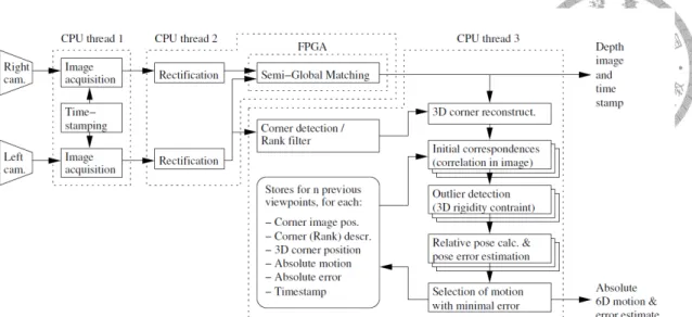
Hirschmuller et al. [6] developed a real-time and accurate ego-motion computation system on a hand-held device attached with stereo cameras and IMU like Figure 2.2 shows.

Their method will generate the depth map based on semi-global matching (SGM) algorithm first, and then use the 2-D corner features and depth information to reconstruct the 3- D corners. Moreover, feature correspondences will be found based on 2-D corners. Next, outlier detection is used to remove the possibly wrong corner correspondences. Finally, the remaining correspondences can be used to calculate the relative pose. The overall scheme is shown in Figure 2.3.

(16)

Figure 2.3: Overall scheme of Hirschmuller et al.’s method

2.3 RGB-D visual odometry

A survey of state-of-the-art RGB-D visual odometry is given by Fang et al. [7]. They divide current RGB-D method into three categories according to what kind of data are mainly used : Image-based [5], [8], [9], Depth-based [10], [11] and Hybrid-based [12], [13], [14].

Next, we are going to introduce a most related work with our system.

Fovis [8] is a vision-based method that estimates the camera motion using depth information for each pixel. It first detects FAST features in color image. Then, the depth corresponding to each feature is extracted from the depth image. Features that do not have an associated depth are discarded. After that, each feature is assigned an 80-byte descriptor. Features are then matched across frames by comparing their feature descriptor values using a mutual-consistency check. Then, the inliers are detected by computing a graph of consistent feature matches and using a greedy algorithm to approximate the maximal clique in the graph. Finally, the motion estimate is computed from the matched features in three steps.

Moreover, a key frame technique is used in Fovis. If the motion relative to the key frame is successfully computed with a sufficient number of inliers, then the key frame is not changed. Otherwise, the current frame replaces the reference frame after the estima-

(17)

tion is finished. If the motion estimation against the reference frame fails, then the motion estimation is tried again with the second most recent frame.

(18)

Chapter 3 Methodology

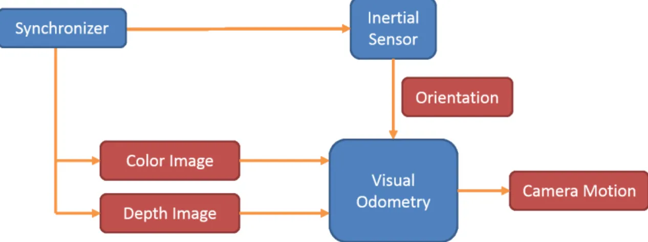
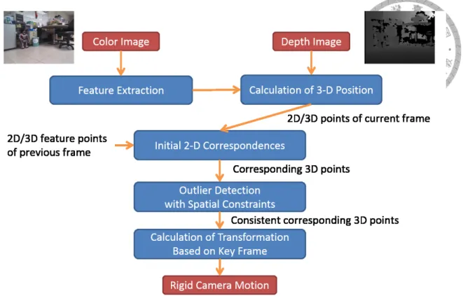
In this section, we introduce our method for ego-motion estimation. Color and depth images are captured from RGB-D camera, and the camera motion can be determined based on visual odometry. Then, the orientation which acquired from inertial sensor fuses with visual odometry to get a more robust estimation. The synchronizer is responsible for synchronizing timestamps on visual and inertial measurements. A system overview is given in Figure 3.1.

Figure 3.1: system overview

3.1 Feature Based Visual Odometry with Spatial Constraints

Since visual odometry is computed incrementally from one frame to the next and every step introduces small errors due to noise. These errors will accumulate to drift at high

(19)

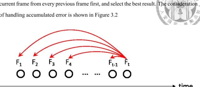
frame rate and then cause negative effect. Hence, we compute the camera motion to the current frame from every previous frame first, and select the best result. The consideration of handling accumulated error is shown in Figure 3.2

Figure 3.2: When the current frame is at time t, then the motion between t and t-1, t and t-2, ... , t and 1 will be computed and select the best one from all results.

For visual odometry, the color images are used to detect the 2-D features and extract feature descriptors using SURF feature [15] first, and then 2-D features are combined with depth information to calculate point clouds in 3-D space. Next, initial correspondences can be derived by matching feature descriptors from the previous and current frame. The initial correspondences are expected to exist a large number of incorrect match pairs, called outliers and these outliers could lead to a bad estimated motion. To avoid this situation, outlier detection is necessary for calculation of the camera motion. Two spatial constraints are used to detect outliers in the set of correspondences. The result of outlier detection is a set of corresponding points, whose satisfied the spatial constraints between each other and the influence of remaining outliers are considered low. Therefore, a singular value de- composition ( SVD ) solution [16] can be used to sufficiently calculate the transformation between two consistent corresponding 3-D point clouds by minimizing the least square error. The accuracy of the estimated transformation is further improved by an iterative optimization method ( e.g. RANSAC [17] ). An overview of visual odometry algorithm is given in Figure 3.3.

(20)

Figure 3.3: Feature Based Visual Odometry with Spatial Constraints

3.2 Feature Correspondences

3.2.1 Initial Correspondences

Figure 3.4: Consideration of Feature Matching

It is assumed that the agent is moving in the static environment, then two corresponding feature points in two different images represent the same 3-D position in the real world.

Feature matching is a good strategy to find the relation between two different images. The consideration of feature matching is shown in Figure 3.4 The SURF detector is applied to detect SURF features first, then extracts feature descriptors. Feature descriptors are used

(21)

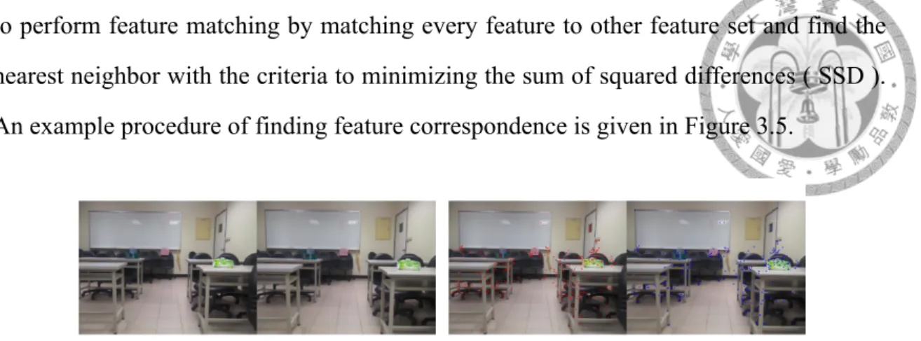
to perform feature matching by matching every feature to other feature set and find the nearest neighbor with the criteria to minimizing the sum of squared differences ( SSD ).

An example procedure of finding feature correspondence is given in Figure 3.5.

(a) There are two input images at different timestamps.

(b) First, the images are used to detect SURF features.

(c) Then, extracting feature descriptors for every detected features.

(d) Finally, finding feature matching by minimizing SSD of descriptors

Figure 3.5: An example of finding feature correspondence.

The correspondence between relevant points from different camera images is required.

It is assumed that there will be a high amount of points, for which no correspondence exists, because some points are outside the field of view of the camera. Furthermore, points can be occluded by objects. It means that SURF detector can fail to detect a feature point in one image, but detects it in the other. Hence, it is not important to find all correspondences.

Theoretically, three none co-linear points are sufficient to calculate the camera motion.

However, a higher amount is useful to increase accuracy, because the effect of noise can be reduced.

3.2.2 2-D to 3-D correspondences

After feature corresponding step, the 3-D feature positions can be derived from 2-D feature points and depth information. It means that the relation between two 3-D point

(22)

(a) (b)

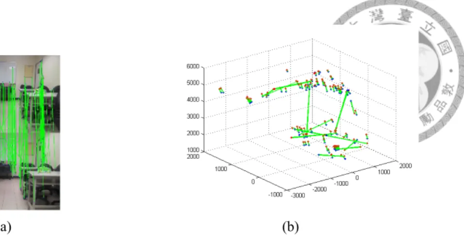
Figure 3.6: An example of correspondences between 2-D matching (left) and 3-D point clouds (right). Every green line means a corresponding pair.

Theoretically, the camera motion can be determined by the corresponding point clouds.

However, there are some feature points exist no correspondences, because they are outside the field of view of the camera or suffer occlusion. Furthermore, there will be a large number of incorrect matching in the correspondences due to the similarity of different feature descriptors like Figure 3.7 shows.

(a) (b)

Figure 3.7: An example of correspondences between 2-D matching (left) and 3-D point clouds (right). Every red line means a incorrect corresponding pair ( i.e. outlier ).

All of the issues mentioned above will lead to an unexpectable estimated motion.

Therefore, it is essential to use some strategies for handling outliers. The rigidity constraints proposed by Hirschmuller et al. [18] are considered as a practicable method to handle these outliers.

(23)

3.3 Outlier Detection

In order to derive a more consistent corresponding set, two spatial constraints are used to remove possibly incorrect correspondence. The initial correspondences step provides a set of corresponding points. The 3-D position in the camera coordinate system can be calculated by combining 2-D position and depth information. The 3-D feature points in the previous and current camera coordinate system are denoted by P_i^t⁻¹ and P_i^t, with corresponding index i and time index t− 1 and t. The motion transformation between two camera coordinate systems is denoted by a rotation matrix R and a translation vector T . The mathematical relation is expressed in equation (3.1). The geometrical bias due to noise in point position is symbolised by b_g_i.

P_i^t⁻¹ = RP_i^t+ T + b_g_i with i = 1...n (3.1) It is expected that there are a large number of outliers in the initial correspondences.

The noise term b_g_iwould become a critical issue for these outliers, the calculation of R and T would derive a bad estimated motion. In most papers, statistics method ( e.g. RANSAC ) is a common way to calculated R and T in the presence of these outliers. However, there are many outliers would be involved in the calculation of transformation. Therefore, we exploit the spatial constraints to efficiently remove most of these outliers, before R and T are calculated.

3.3.1 Relative Distance Constraint

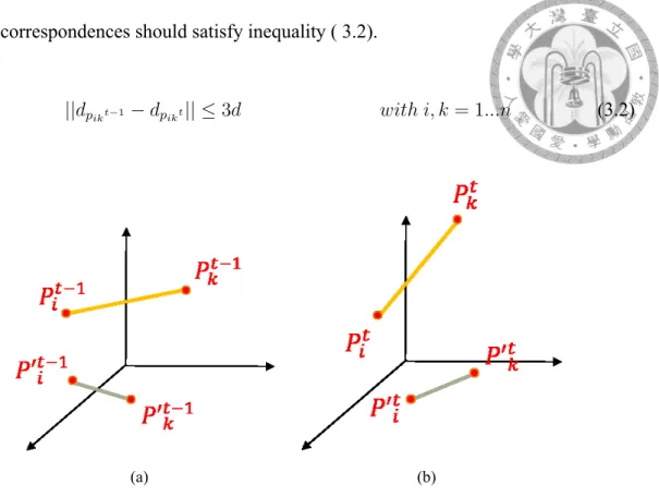
The first constraint is the relative distance between two 3-D points should remain unchanged under a rigid transformation. Therefore, the distance between any two points d_p_ik^t−1 =||Pit−1− Pkt−1|| should be the same for the corresponding points dpikt =||Pit− Pkt||.

Hence, we set a small d represents the difference between two relative distance. All of the feature correspondences should satisfy inequality ( 3.2 ).

Hirschmuller et al. [19] have showen that how models the image based errors and

(24)

feature correspondences should satisfy inequality ( 3.2).

||dpikt−1− dpikt|| ≤ 3d with i, k = 1...n (3.2)

(a) (b)

Figure 3.8: The relative distance between P_i and P_k should be the same at time t and t− 1 ( i.e. the length of orange line keeps unchanged ). Similarly, the gray line also keeps unchanged.

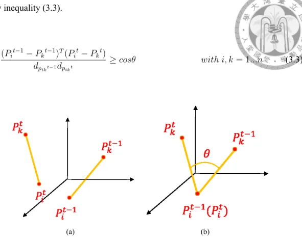
3.3.2 Rotation Angle Constraint

The second constraint is derived by setting an upper bound θ on the rotation angle of the camera between consecutive images. The rotation angle is limited by a high frame rate (e.g. 30 fps). That is, camera wouldn’t suffer a large rotation movement within 1/30 sec (i.e. between two consecutive images). Mathematically, all rotations in three dimensions can be represented by a rotation axis and a rotation angle. If the vector P_i^t⁻¹− Pkt−1

is orthogonal to the rotation axis, then the angle between P_i^t⁻¹− Pkt−1 and P_i^t− Pkt

matches exactly the rotation angle. If P_i^t⁻¹− Pkt−1 is parallel to the rotation axis, then the angle between P_i^t⁻¹− Pkt−1 and P_i^t− Pktis always 0. In all other cases, the angle is in between 0 and the rotation angle. The rotation axis is unknown, but the angle is limited by θ as described above. Therefore, all pairs of correct correspondences must

(25)

satisfy inequality (3.3).

(P_i^t⁻¹− Pkt−1)^T(P_i^t− Pkt)

d_p_ikt−1d_p_ik^t ≥ cosθ with i, k = 1...n (3.3)

(a) (b)

Figure 3.9: A vector ⃗a = P_i^t⁻¹− Pkt−1 is formed by two 3-D points P_i^t⁻¹ and P_k^t⁻¹ at time t− 1. This vector becomes vector ⃗b = Pit− Pktby suffering a transformation at time t (left). The rotation angle constraint is setting a limitation of the angle θ between vector ⃗a and ⃗b (right).

3.3.3 Consistent Subset of Correspondences

The initial correspondence of matching pairs can be validated by check both con- straints. If there is a pair (i, k) of corresponding matching pairs (P_i^t−1, P_i^t) and (P_k^t−1, P_k^t) satisfies both constraints, then both correspondences may be correct. If one of the constraints doesn’t satisfy, then at least one of the correspondences in the pair is abso- lutely wrong. Although we cannot determine that which one would be the wrong correspondence. However, these information can be used to construct a consistent table of corresponding points. Each entry in the table represent whether the corresponding matching pairs satisfy both constraints. If some pairs satisfy both constraints , then the entry will equal to one. Otherwise, entry in the table will be filled in zero. Figure 3.10 visualizes an example of consistent table. After we construct a consistent table, our goal is to find a

(26)

Figure 3.10: An example of the consistent table.

Theoretically, we want to find out the largest subset would involve testing all the combinations of n points with 2ⁿ possibilities, but it is obvious that this task is not be a practical issue. Actually, in real usage, it is not necessary to find the largest subset, but only a large enough subset. The first thing is selecting the point i with the largest number of consistencies (i.e. the column i with the largest number of 1-elements) and putting into the consistent subset. Then, selecting another point into subset insures that the consistencies are maintained for all points in the subset. Repeating this procedure until there are no other points can be added into subset. In the Figure 3.11, a 5× 5 consistent table example is given to demonstrate how to find the consistent subset by using the scheme mentioned above.

Although we perform an outlier detection procedure, it may remain incorrect correspondences. However, the remaining outliers also satisfies the distance and rotation constraints ( 3.2 ) and ( 3.3 ). We can expect that the influence of remaining outliers would be small. Therefore, these errors can be well handled during calculation of R and T . The results of original matching and matching after removing outliers are shown in Figure 3.12.

(27)

(a) A 5× 5 A consistent table which the en- tries have been filled with 0 or 1.

(b) First, we select the column with most 1- elements ( second column in this example ).

(c) Adding the second corresponding pair into subset.

(d) Finding next corresponding pair ( e.g.

third pair ) is consistent with second pair.

(e) Checking the consistencies between third pair and all pairs in subset.

(f) If the consistencies satisfied, then adding the third pair into subset.

(g) Repeating the same steps, then the forth pair is also added into subset.

(h) Next, finding corresponding pair ( e.g.

fifth pair ) is consistent with second pair.

(i) Checking the consistencies between fifth pair and all pairs in subset.

(j) Since the consistencies don’t satisfy, the fifth pair is not added into subset.

Figure 3.11: A 5× 5 example to show how to finding the consistent subset.

(28)

(a) original matching result

(b) matching result after outlier detection

Figure 3.12: feature matching results

3.4 Motion Estimation

Figure 3.13: Motion Estimation Scenario

A camera moving in the static environment can be viewed as the camera is fixed and the feature points suffer the movements in opposite direction. Therefore, the camera

(29)

motion R, T between consecutive images can be calculated from the set of consistent correspondences. With the transformation described in equation (3.1), the least squared error can be used to estimate the camera pose by minimizing equation (3.4). The initial solution is solved by SVD, and then refines the solution by RANSAC. The scenario of motion estimation is shown in Figure 3.13.

∑k

i=1

||Pit− (RPit−1+ t)||² (3.4)

3.5 Fusion with Inertial Measurement Unit

Visual odometry, which determine camera motion according to the associated camera images, gives accurate estimation of translatory movement, but it is possibly inaccurate to estimate the rotational movement. Therefore, an inertial measurement with accurate rotational estimation would be useful for justifying the rotational error generated in the visual odometry. We acquire inertial measurements from inertial sensor to compute an initial rotation, then estimating camera motion by minimizing sum of squared error between two 3-D point clouds. The fusion scheme is described below.

step1 : random sample 10 corresponding points B ={Pit−1, P_i^t} for i = 1, 2, ..., 10 from corresponding point clouds A ={Pit−1, P_i^t} for i = 1, 2, ..., n

step2 : compute camera motion using sampling points and initial orientation derived from inertial sensor by equation 3.5

t = 1 10

∑10

i=1

P_i^t− R 1 10

∑10

i=1

P_i^t⁻¹ (3.5)

step3 : calculate the re-projection error defined by equation 3.6

∑

{Pit−1,Pit}∈A\B||Pit− (RPit−1+ t)||² (3.6)

(30)

imal re-projection error

3.6 Key Frame Selection

As mention in section 3.4, since visual odometry is computed incrementally between two consecutive images and every step produces tiny errors due to noise, these errors will accumulate to a non-negligible drift at high frame rate. Nevertheless, if the frame rate is too slow for the local camera motion, it is difficult to find enough correspondences for motion estimation, which also degrades the performance. Hence, we compute camera motion to the current frame from every previous frame to reduce the influence of accumulated error. However, computing motion to the current frame from every previous frame is time- consuming. Thus, we compute the motion to the current frame from n previous frames that called key frames, where n is a pre-defined, fixed number ( 5 in our experiments).

The overall motion error from current frame to one of key frames can be calculated by equation 3.7. The motion with minimal overall motion error would be chosen as the final 6-D motion. The new frame replaces the one with the highest overall motion error in the list of n key frames. With this strategy, it mitigates the influence of accumulated error.

∑n

i=1

||Pit0 − (RPitk + t)||²+

∑n

i=1

||Pitk− (RPit+ t)||² (3.7)

(31)

(a) (b)

(c) (d)

(e) (f)

(g)

Figure 3.14: For computing the motion of F_n, we calculate the motion to F_n from KF₁ KF₅. Then, selecting the motion with minimal overall motion error and replacing the key frame with highest overall motion error.

(32)

Chapter 4 Experimental Results

In this section, we evaluate the performance of our ego-motion estimation algorithm in several experiments with no prior knowledge of camera motion and environment. Our approach is tested by image sequences contains only translatory motion or rotational motion first, and demonstrate the accuracy of the algorithm. Then, we compare the results between visual results and fusion results to verify that IMU can really improve the performance of motion estimation. Finally, we take several turn rounds in different seminar rooms to show the robustness of our method.

4.1 Experimental Setup

Figure 4.1 shows our ego-motion estimation agent. A Microsoft Kinect v1 with a resolution of 640 x 480 pixels and an Oculus Rift integrating a triaxial accelerometer, gyroscope and magnetometer are attached on a sliding chair. When the agent is moving in a static environment, the color and depth information will be captured by Kinect and the inertial measurement will be acquired by Oculus Rift. Two scenes of the testing rooms are shown in Figure 4.2. The camera motion is determined by those data.

(33)

(a) (b)

Figure 4.1: The ego-motion estimation device

(a) (b)

Figure 4.2: Two scenes of the testing rooms

4.2 Effect of Outlier Detection

An example sequence that consists of 600 images has been captured with our system. The camera has basically been moved in 360^◦circle. The diagram on the Figure 4.3 demonstrates the power of the method to discriminate outliers from the initial correspondence set.

(34)

Figure 4.3: The number of initial correspondences, consistent correspondences and remaining inliers after RANSAC between two images.

4.3 Translatory Motion Experiments

Some simple cases are performed to test our algorithm can cope with translatory motion correctly.

In these experiments, the agent moved forth about 3 meters and back, then the camera motion was calculated by the visual and inertial readings. Figure 4.4 shows the estimated motion sequences and demonstrates the ability to robustly estimate the translatory motion by fusing visual and inertial measurements. The detail estimated data are given in Table 4.1. A 4.6% average error rate is achieved by using the fusion algorithm.

−1500 −1000 −500 0 500 1000 1500

0 500 1000 1500 2000 2500 3000 3500

Figure 4.4: Estimated result with translatory motion only

(35)

Table 4.1: Evaluation of Translation Test Translation Distance Ground Truth Estimated

Results Run 1 ∼ 3 meters 2.86 meters Run 2 ∼ 3 meters 2.71 meters Run 3 ∼ 3 meters 2.95 meters Run 4 ∼ 3 meters 2.93 meters Run 5 ∼ 3 meters 2.84 meters Average ∼ 3 meters 2.86 meters

4.4 Comparison of visual results and fusion results

Visual odometry, which determine camera motion according to the associated camera images, gives accurate estimation of translatory movement, but it is possibly inaccurate to estimate the rotational movement. In contrast, the Inertial Measurement Unit, which determine camera motion by integrating the measurements from accelerometers, gyroscopes and magnetometers, provides accurate orientation estimation, but produces drift in long- term translation estimation due to the integration noise. Therefore, combining visual and inertial measurements has complementary properties which make a more robust motion estimation for many robotic applications.

We have chosen a round trips way in room 324 at our institute for comparing the influence of fusion with inertial measurement. The experimental results are shown in Fig- ure 4.5. We get the travelled distances about 11.8 m and 14.2 m and are in the end 1.1 m and 0.3 m away from camera’s initial position, respectively.

(36)

(a) visual odometry alone (b) fusion with inertial measurements

Figure 4.5: Estimated results of a turn round trip

It can be seen that computing visual odometry alone is inferior to using the fusion method. That is, fusion with inertial data is really useful for improving the performance of motion estimation.

4.5 Long-term Round Trip Experiment

Another experiment is a round trip way through a part of corridor in our institute for testing the robustness of our system. The estimated results are shown in Figure 4.6. The red trajectory is visual alone result and the blue trajectory is fusion result. Moreover, we compare our result with other ego-motion estimation method mentioned in section 2 using the loop-closing error criteria. The comparison results is shown in Table 4.2. The loop- closing error is the distance in the end of trajectory away from the start position divides by the total distance of the trajectory.

(37)

Figure 4.6: Estimated results of long-term round trip. The red trajectory is the visual alone result, the blue trajectory is the fusion result and the green trajectory is the ground truth. The total distance of blue and red path are 142.9 m and 116.3 m, respectively. The manually measured ground truth is 119.7 m.

Table 4.2: Comparison with other methods Method Trajectory

Error Loop-closing

Distance Error

Kneip et al.’s 22.59 meters 0.6 meters 2.66 % Hirschumller et al.’s 140 meters 0.61 meters 0.44 % Ours 119.7 meters 8.7 meters 7.27 %

(38)

Chapter 5 Conclusion and Future Work

A system proposed in this thesis for visual-inertial-based ego-motion estimation starts from feature correspondences, goes through fusion with inertial data to robust camera motion computation.

In the feature correspondences part, SURF features are extracted for feature matching usage first, then two spatial constraints are applied to efficiently remove outliers, and get consistent corresponding 3-D point clouds through a procedure of complexity handling.

Camera motion estimation utilize consistent corresponding 3-D point clouds with statistic optimization method for outlier handling, the inertial measurement is involved in this step as initial setting. The accumulated drift problem due to the noise of consecutive images is also concerned by a key frame technique.

The test in Section 4.3 shows that the algorithm can estimate translatory movements correctly. With an accurate initial rotation value, it is also shown that the estimated motion will be more accurate in Section 4.4. Section 4.5 demonstrates that our system can estimate different camera movements robustly in real round trip data.

In the future, we plan to improve accuracy by revising the key frame selection technique. A more suitable key frame can be found by comparing the viewpoints between current frame and frames in the whole past track. With this strategy, the camera motion can be estimated using two images which having similar viewpoints. We expect that new key frame technique will be useful for feature matching and benefits to the final result.

With an accurate performance for ego-motion system, we see a great potential applica-

(39)

tion for drone control and navigation. It is also suitable for augmented reality applications on head-mounted display.

(40)

Bibliography

[1] Andrew J Davison. Real-time simultaneous localisation and mapping with a single camera. In Computer Vision, 2003. Proceedings. Ninth IEEE International Confer- ence on, pages 1403–1410. IEEE, 2003.

[2] Davide Scaramuzza and Friedrich Fraundorfer. Visual odometry [tutorial]. Robotics

& Automation Magazine, IEEE, 18(4):80–92, 2011.

[3] David Nistér, Oleg Naroditsky, and James Bergen. Visual odometry. In Computer Vision and Pattern Recognition, 2004. CVPR 2004. Proceedings of the 2004 IEEE Computer Society Conference on, volume 1, pages I–652. IEEE, 2004.

[4] Laurent Kneip, Margarita Chli, Roland Siegwart, Roland Yves Siegwart, and Roland Yves Siegwart. Robust real-time visual odometry with a single camera and an imu. In BMVC, pages 1–11, 2011.

[5] Andreas Geiger, Julius Ziegler, and Christoph Stiller. Stereoscan: Dense 3d recon- struction in real-time. In Intelligent Vehicles Symposium (IV), 2011 IEEE, pages 963–

968. IEEE, 2011.

[6] Korbinian Schmid and Heiko Hirschmuller. Stereo vision and imu based real-time ego-motion and depth image computation on a handheld device. In Robotics and Au- tomation (ICRA), 2013 IEEE International Conference on, pages 4671–4678. IEEE, 2013.

[7] Zheng Fang and Yu Zhang. Experimental evaluation of rgb-d visual odometry meth- ods. International Journal of Advanced Robotic Systems, 12, 2015.

(41)

[8] Albert S Huang, Abraham Bachrach, Peter Henry, Michael Krainin, Daniel Matu- rana, Dieter Fox, and Nicholas Roy. Visual odometry and mapping for autonomous flight using an rgb-d camera. In International Symposium on Robotics Research (ISRR), pages 1–16, 2011.

[9] Christian Kerl, Jurgen Sturm, and Daniel Cremers. Robust odometry estimation for rgb-d cameras. In Robotics and Automation (ICRA), 2013 IEEE International Conference on, pages 3748–3754. IEEE, 2013.

[10] François Pomerleau, Francis Colas, Roland Siegwart, and Stéphane Magnenat. Com- paring icp variants on real-world data sets. Autonomous Robots, 34(3):133–148, 2013.

[11] Graeme Jones. Accurate and computationally-inexpensive recovery of ego-motion using optical flow and range flow with extended temporal support. In Procedings of the British Machine Vision Conference 2013, pages 75–1, 2013.

[12] Henrik Andreasson and Todor Stoyanov. Real time registration of rgb-d data using local visual features and 3d-ndt registration. In SPME Workshop at Int. Conf. on Robotics and Automation (ICRA), 2012.

[13] Ivan Dryanovski, Roberto G Valenti, and Jizhong Xiao. Fast visual odometry and mapping from rgb-d data. In Robotics and Automation (ICRA), 2013 IEEE Interna- tional Conference on, pages 2305–2310. IEEE, 2013.

[14] Ji Zhang, Michael Kaess, and Sushil Singh. Real-time depth enhanced monocular odometry. In Intelligent Robots and Systems (IROS 2014), 2014 IEEE/RSJ Interna- tional Conference on, pages 4973–4980. IEEE, 2014.

[15] Herbert Bay, Tinne Tuytelaars, and Luc Van Gool. Surf: Speeded up robust features.

In Computer vision–ECCV 2006, pages 404–417. Springer, 2006.

[16] Robert M Haralick, Hyonam Joo, Chung-Nan Lee, Xinhua Zhuang, Vinay G Vaidya,

(42)

[17] Martin A Fischler and Robert C Bolles. Random sample consensus: a paradigm for model fitting with applications to image analysis and automated cartography.

Communications of the ACM, 24(6):381–395, 1981.

[18] Heiko Hirschmuller, Peter R Innocent, and Jon M Garibaldi. Fast, unconstrained camera motion estimation from stereo without tracking and robust statistics. In Con- trol, Automation, Robotics and Vision, 2002. ICARCV 2002. 7th International Con- ference on, volume 2, pages 1099–1104. IEEE, 2002.

[19] Annett Stelzer, Heiko Hirschmüller, and Martin Görner. Stereo-vision-based navi- gation of a six-legged walking robot in unknown rough terrain. The International Journal of Robotics Research, 31(4):381–402, 2012.