Abstract—Downlink broadcast in LTE-Advanced and WiMAX-based relay networks is a crucial service for multimedia delivery. Currently most research effort goes into devising efficient resource allocation mechanisms to achieve more efficient resource utilization. However, spatial reuse, an important technique to improve transmission capacity, has received little attention in the literature. Thus, in this work, we investigate ways of achieving more efficient resource allocation in wireless relay networks via spatial reuse. We first formulate a joint spatial reuse and resource allocation problem as an integer linear programming (ILP) model. We then consider a grouping mechanism in which relay stations (RSs) are grouped together if they do not interfere with each other’s transmission signal. RSs in the same group can thus utilize spatial reuse by using the same set of resources to broadcast data. Because of the high computational complexity of ILP model, we propose a two-phase heuristic solution. In the first phase, the Enhanced-Resource Diminishing Principle approach is employed to determine the number of resources required by the base station and a set of selected RSs. In the second phase, a Max-Coloring algorithm is employed to organize the selected RSs into broadcast groups and then assign the required resources to each group by exploring the maximum advantage of spatial reuse. The simulation results show that the proposed solution improves system performance up to 61% as compared to two existing mechanisms.
Index Terms—broadcast, conflict graph, graph coloring, path construction, relay networks, resource allocation, spatial reuse.
I. INTRODUCTION
HE very rapid spread of smart phones has generated an increasing demand for delivering multimedia content over wireless networks. Two leading standards, 3GPP LTE-Advanced and IEEE 802.16m WiMAX, provide high data transmission rates for real-time multimedia applications (e.g., Internet Protocol Television (IPTV) or video conferencing) that Manuscript received April 13, 2014; revised September 25, 2014, November 13, 2014; accepted November 17, 2014. This work was supported in part by the Ministry of science and technology under Grant 103-2221-E-194 -022 -MY2.
C. H. Lin, R. H. Hwang, J. J. Wu, J. F. Lee are with Department of Computer Science and Information Engineering, National Chung Cheng University, Chia-Yi, Taiwan, R.O.C. (e-mail: vexonelit@gmail.com;
rhhwang@cs.ccu.edu.tw; wcc101p@cs.ccu.edu.tw, jflee@cs.ccu.edu.tw).
Y. D. Lin is with Department of Computer Science, National Chiao Tung University, Hsinchu, Taiwan, R.O.C. (e-mail: ydlin@cs.nctu.edu.tw).
Corresponding Author: R.H. Hwang (rhhwang@cs.ccu.edu.tw)
need to transmit massive amounts of data. However, it is less likely that a single base station (BS) could cover a large geographic area while providing mobile stations with high data transmission rates. As a consequence, adding smaller cells into the macrocell architecture becomes the direction of the next-generation wireless networks. In particular, both LTE-A and WiMAX have adopted RSs as one of the small cell solutions [1]. RSs, by collaborating with the BS, can improve the overall throughput and coverage [2]-[3]. A RS can operate in a transparent or a non-transparent mode. A transparent relay mode increases the throughput but cannot extend BS coverage area. On the other hand, a non-transparent relay mode is used to extend the coverage area of a BS [4]. In this work, we assume that a non-transparent mode is adopted and refer to such a network as a wireless relay network.
As more and more operators invest in mobile IPTV service [5], the access networks face the challenge of transmitting video streams to mobile users in real-time, which is a very high bandwidth-consuming service [6]. Broadcast service is a downlink point-to-multipoint access service which transmits a single copy of multimedia data to all users within a cell.
Obviously, this kind of push-type service offers a more efficient way of utilizing bandwidth for providing mobile IPTV service. We thus focus on the downlink broadcast service in a wireless relay network. As in most of the literature, we mainly focus on the network model of a single cell which typically comprises one BS, multiple RSs, and multiple mobile stations (MSs). We consider a case where the MSs subscribe to a real-time multimedia program, e.g., a mobile IPTV channel. An MS can receive data either from the BS directly or via an RS relaying data to it. That is, we only consider a two-hop wireless relay network. Before delivering data to MSs, an RS must receive a copy of the data from the BS.
For a broadcast service, a wireless relay network needs to decide not only on the data relaying path, but also on the number of resources that should be reserved for the transmission once a broadcast session is triggered. The number of the resources required for a successful transmission between a sender and a receiver depends on the modulation and coding scheme (MCS) chosen in response to the channel condition.
The unit of resource could be a time slot in WiMAX or a resource block (RB) in LTE-A. Once the MCS has been determined, the amount of data that could be transmitted per unit of resource can also be determined. If the amount of real-time multimedia data to be broadcasted is
M
(per unit ofIntegration of Spatial Reuse and Allocation for Downlink Broadcast in LTE-Advanced and
WiMAX Relay Networks
Cheng-Hsien Lin, Ren-Hung Hwang, Jang-Jiin Wu, Jeng-Farn Lee, and Ying-Dar Lin
T
time) and the data rate per unit of resource is b, it thus requires
M
/b
units of resource per unit of time for the broadcast service.In addition, the broadcast data must be received by all MSs in the sender’s (a BS or RS) transmission range, and the choice of MCS will affect whether a MS can successfully receive the broadcast data or not. There is thus a tradeoff between the MCS and the number of MSs that successfully received the broadcast data. A more robust MCS require more resource units to transmit the broadcast data but ensures more MSs that can successfully receive the broadcast data. It is crucial that the resource is utilized efficiently to deliver real-time multimedia data to all the designated MSs, since the radio resource is shared by all network components in the same cell. One way to achieve this goal is to properly select the MCS settings for the base station (BS) and a set of selected relay station (RSs), and then allocate to them the required resources to build a set of data relaying paths that connect the BS with all the designated MSs. In addition, spatial reuse could be used to further improve the resource efficiency. That is, the same set of resources can be used by a group of RSs, rather than by a single RS, as long as the RSs are able to broadcast data concurrently, without any mutual interference. The features of these two approaches motivated us to seek a solution that addresses spatial reuse and resource allocation simultaneously.
We use the example shown in Fig. 1 to further clarify the problem: here two allocation strategies are separately applied on a relay network of 1 BS, 8 RSs, and 12 MSs. Fig. 1(a) shows that RS5, RS6, RS7, and RS8 are selected to cooperate with the BS and are allocated 6 units of resource (including the BS).The allocation strategy in Fig. 1(b) selects RS1, RS2, RS3, and RS4 as relay nodes and allocates every selected RS 1 unit of resource. In the absence of spatial reuse, the total amount of required resources in Fig. 1(b) is 10 units, less than the 30 units of resources required by the allocation strategy in Fig. 1(a). The resource efficiency can be raised further if the gain of spatial reuse is exploited. As shown in Fig. 1(a), 12 units of resources can be saved if the four RSs are evenly arranged in two broadcast groups (i.e., RS5 and RS7 form a group, and RS6 and RS8 form another group), where two RSs within a group share the assigned 6 units of resources. Similarly, RS1, RS2, RS3, and RS4 in Fig. 1(b) form a single broadcast group to increase efficiency by 30% by reusing the assigned 1 unit of resource.
From this example, it is clear that the combination of spatial reuse and resource allocation provides opportunity to improve overall resource efficiency. However, how to compute the optimal solution for the problem is a daunting task because of the following two aspects. First, selecting a different set of RSs yields different resource requirement for the broadcast transmission. Second, the interference relationship among the selected RSs affects the efficiency of spatial reuse. The objective then is to minimize resource allocation within the constraints that every broadcast group demands a different number of resources and that spatial reuse posts limitation on channel usage. In an attempt to address these issues, this paper first formulates the joint spatial reuse and resource allocation (JSRA) problem using an integer linear programming (ILP) model. Unfortunately, using the ILP to obtain the optimal solution incurs high computational costs and is difficult to put
into practice for general use. Nevertheless, this paper treats the JSRA problem in two computation stages and employs a
sub-optimal algorithm for each stage. The purpose of the first stage is to determine the number of resources required for the BS, and a set of selected RSs, while ensuring that all the designated MSs can receive the broadcast data either directly from a BS or indirectly via an RS. In the second stage, the purpose is to form a set of broadcast groups and then assign the required resources to each group.
In this paper, we propose the Enhanced-Resource Diminishing Principle (E-RDP) algorithm for the first stage, and adopt the Max-Coloring (MXC) algorithm [7] for the second stage. Performance of the proposed mechanism is evaluated by extensive simulations. Our simulation results indicate that by integrating E-RDP and MXC, the overall performance can be improved by as much as 61% compared to the Broadcast Incremental Power (BIP) mechanism [8] and a utility-based approach [9].
The remainder of this paper is organized as follows. Section 2 discusses related work. Section 3 describes the system model and the notations used in the paper. This section also presents the ILP model of the problem we address. In Section 4, we explain the details of E-RDP and MXC algorithms. Simulation results are presented in Section 5. In conclusion we envision some future directions in Section 6.
II. RELATED WORK
This section reviews three aspects of current studies: 1) video multicast over wireless networks; 2) the resource allocation for downlink broadcast over multi-hop wireless networks; and 3) the spatial reuse over multi-hop wireless networks.
A. Multicast scheduling for OFDMA networks
Early works on multicast in wireless networks mainly focused on the resource allocation for delivering layered video over the multicast channel [10]-[12]. Most of them address the issue of how to allocate resources to different layers of videos so that the quality of the video received or revenue of the system can be optimized. For example, in [10], the multicast resource allocation problem was modeled as an optimization problem and a greedy algorithm was proposed to maximize total utility. A utility-based resource allocation scheme was proposed in [11] which tried to allocate resources to the base layer of all videos first and allocated resources to enhancement layers by maximizing marginal utility. In [12], an opportunistic
(a) (b)
Fig. 1. Illustration of the problem addressed in this study.
RS2
MS2
MS1 MS3
MS4 MS5
MS6
MS7
MS8
BS MS9
MS10 MS11 MS12
1 unit 6 units
1 unit
1 unit 1 unit
RS1
RS4
RS3 RS2
RS5
RS6 RS7
RS8
RS2
MS2
MS1 MS3
MS4 MS5
MS6
MS7
MS8
BS MS9
MS10 MS11 MS12 RS1
RS4
RS3
6 units 6 units
6 units
RS6 RS5
RS7 RS8 6 units
multicasting concept was proposed in which user scheduling and resource allocation was jointly considered. In addition, an FEC rate adaptation scheme was also presented to improve resource utilization. However, a relay station technique was not considered in these works.
B. Resource allocation for downlink broadcast over multi-hop wireless networks
Studies [9], [13]-[14] investigated the broadcast recipient maximization problem under a constraint of limited resource.
Given all resource requirements (i.e., the number of resources required by a sender to serve a receiver successfully) of the network, [9], [13]-[14] investigated how to have a network serve as many recipients (in our context, i.e., the MSs) as possible by allocating a limited number of resources to the BS and a subset of RSs efficiently. The problem considered in [13]
requires a given network topology (i.e., each MS as known to receive data from a designated sender) as input, whereas the problem considered in [14] assumes that the set of recipients a sender can serve depends upon the number of resources assigned to the sender. Unlike the studies in [13]-[14] which only consider 2-hop relay networks, the work in [9] addresses the problem via a multi-hop relay networks. Notably studies [13]-[14] are highly related to our work since we share the same problem formulation and network model.
Minimizing energy for broadcasting in wireless ad-hoc networks (also known as mesh networks) is a well-studied issue [15]-[24]. Any node can act as a traffic relay node in such networks. The commonly-adopted solution to this matter is to construct a broadcast tree rooted at the source node and connecting to the rest of nodes in the network, while minimizing the energy consumption of the nodes that take part in broadcasting data.
In summary, the scope of works in this category merely concentrates on addressing the resource allocation problem.
However, this paper extends the problem to embrace spatial reuse issue as well. As a result, this principal difference forms a barrier that limits the existing problem models and solutions from responding to the new challenge.
C. Spatial reuse over multi-hop wireless networks
Researchers [25]-[26] investigated how to improve network throughput via spatial reuse in wireless mesh networks. Their common objective was to find an optimal schedule in which a number of given communication links is arranged into a number of time slots such that the total number of required time slots is minimized. Spatial reuse was exploited to improve network throughput when interference-free links can be scheduled at the same set of time slots. Sundaresan and Rangarajan [27]-[29] investigated the resource allocation of a two-hop wireless relay network. A set of OFDM channels was assigned to a set of given relay links (BS-RS) and access links (RS-MS) in order to maximize the average user throughput.
Different relay links and access links that do not cause mutual interference can be scheduled on the same set of OFDM channels to take advantage of spatial reuse. Cooperative transmission is also considered in [29] to further improve the throughput. In [30], resource allocation problem for multicast IPTV service in relay-assisted centralized wireless access networks was studied. In order to take the advantage of spatial
reuse, RSs were divided into R non-interfering groups and transmission slots of RSs were scheduled so that either all of the RSs within the group transmitted simultaneously, or none of them transmitted at all. Similarly, in [31], spatial reuse was considered in multicast scheduling of mini-slot in IEEE 802.16 mesh networks. The authors proposed a downlink interference-aware scheduling algorithm for transferring multicast data in which relay stations may have concurrent transmission.
In summary, previous work in this category focused on improving system utilization through spatial reuse. However, all these works differ from our work in some of the following aspects. First, some considered mesh networks [25]-[26] in which any mobile node can act as a relay node, while we make a distinction between a mobile node and a relay station. Second, some placed emphasis on either OFMDA channel scheduling [27]-[29] or on the formation of a multicast tree in mesh networks [31], while we focus on the resource allocation issue.
Finally, some assumed that network topology is known a priori.
For example, [27] assumed that the set of interference-free relay groups is given in the problem formulation. In our work, we do not make such an assumption. Instead, we propose an E-RDP algorithm to determine the set of RSs that will first participate in the broadcast service. The use of spatial reuse to improve system utilization is then solved by the MXC algorithm.
III. SYSTEM MODEL AND ILPFORMULATION A. System Model and Notations
This paper considers a wireless relay network of one BS, N RSs, and M MSs. Each device is assigned with an identification (ID) number as follows: let the ID of the BS be 0, the IDs of the RSs range from 1 to N, and the IDs of the MSs range from 1 to M. The BS is responsible for scheduling downlink requests for data transmissions (from the BS to the RSs or MSs, and from the RSs to MSs) centrally, and for informing the RSs and MSs of the scheduled results.
In a relay network, real-time multimedia streaming is assumed to be broadcast from the BS to all MSs. An MS receives the broadcast data either directly from the BS or indirectly from an RS, depending on the result derived from the JSRA problem. To establish data paths for multimedia delivery, the system must find a set of broadcast groups and allocate different number of resources to them appropriately. The broadcast group in this paper is a logical entity used to represent a group of senders that can concurrently broadcast data to a subset of MSs. That is, simultaneous transmissions of these senders will not interfere with each other [31]. When the number of senders within a broadcast group exceeds one, spatial reuse is achieved since they utilize the same set of resources to broadcast data. Disjointed sets of resources are assigned to different broadcast groups so that they broadcast data in turn to avoid interference between groups. The resource requirement of a broadcast group is the minimum number of resources required to transmit the streaming data to all of its serving receivers (MSs) with required QoS. A broadcast group either contains the BS itself only, or a set of interference-free RSs. An RS, if selected as a relay station, is allowed to appear in exactly one broadcast group only.
This paper regards the radio resource as a general form which denotes any type of resource used in existing radio technologies. For example, both LTE-A or WiMAX adopt OFDMA as their multiple access mechanism. The resource in this context refers to the total number of resource blocks used to broadcast the streaming data. The resources required for a downlink transmission between a sender i (i.e., the BS or an RS) and a receiver j (i.e., an RS or an MS) is denoted by di,j, which is determined by the MCS chosen by i in response to the channel condition feedback from the receiver j. This paper defines three vectors DBR, DBM, and DRM to maintain information of the required resources of a sender. The notations DBR [𝑑0,1𝑅 , 𝑑0,2𝑅 , …, 𝑑0,𝑁𝑅 ] and DBM [d0,1, d0,2, …, d0,M] are row vectors while the notation DRM [D1, …, DN]T is a two dimensional matrix, where Dn [dn,1, dn,2, …, dn,M].
To take advantage of spatial reuse, a broadcast group is formed by interference-free RSs. In this work two RSs are defined as interference-free if there is no MS that can receive radio signals from both RSs. We use the notation xn,m to denote whether MS m can receive the signal emitted from RS n. If MS m receives RS n’s signal, then xn,m 1; otherwise, xn,m 0. All the information related to xn,m is kept in the matrix RM [1, …, n, ..., N]T, where n [xn,1, …, xn,m, …, xn,M]. Table I lists the notations used throughout the paper.
B. Integer Linear Programming Model for JSRA
In this section, essential variables used in the proposed integer linear programming (ILP) model are presented. First, decision variables 𝑢0,𝑖𝑅 and ui,m represent if the broadcast data has been successfully transmitted from a certain sender to a specified receiver. The binary variable 𝑢0,𝑖𝑅 {0, 1} (1 i N) denotes whether RS i receives a copy of broadcast data from the BS. Similarly, the binary variable ui,m {0, 1} (0 i N, 1 m
M) denotes whether MS m can receive a copy of broadcast data from sender i. We also define the binary variables zi,m {0, 1} (0 i N, 1 m M) to indicate if MS m is designated to receive broadcast data from sender i. When the sender is the BS (i 0), we have zi,m u0,m. Otherwise, the sender is an RS, and zi,m 𝑢0,𝑖𝑅 ui,m which indicates the broadcast data is transmitted to RS i first, and then related to MS m.
Next, we define the decision variables representing the interference relation between a pair of RSs. The binary variable ci1,i2,m {0, 1} denotes whether MS m is subject to receive interfering signals from RSs i1 and i2. The binary variable ci1,i2
{0, 1} simply denotes whether interference takes place between RSs i1 and i2. Furthermore, the binary variable gi,k {0, 1} indicates if the k-th unit of resource is assigned to RS i. This set of decision variables is used to determine how to allocate resource to broadcast groups. To evaluate the ultimate result of JSRA, we also define the following two variables: 1) the variable Yi
Z
(0 i N) represents the number of resources allocated to sender i; 2) the binary variable sk {0, 1} (1 k L) indicates if the k-th unit of resource is allocated for broadcast.Given the channel conditions of wireless networks (i.e., DBR, DBM, and DRM) and the signal coverage sets for all the RSs (i.e.,
RM), the goal of the JSRA problem is to find a set of best broadcast groups, so that the total number of resources
allocated to these groups is minimized under the constraint that the broadcast service is received by all MSs. The ILP for JSRA is formulated as follows:
minimize Y0Lk1
s
k,
(1)subject to
Y0 𝑢0,𝑛𝑅 𝑑0,𝑛𝑅 0, 1 n N, (2) Yi zi,m di,m 0, 0 i N, 1 m M, (3)
i zi,m 1, 1 m M, (4)
ci1,i2,m xi1,m xi2,m [1 (1 zi1,m)(1 zi2,m)],
1 i1, i2 N, 1 m M, (5)
ci1,i2 ci1,i2,m, 1 m M, (6)
gi1,k gi2,k 2 ci1,i2, 1 i1, i2 N, 1 k L, (7) sk gi,k, 1 i N, 1 k L, (8)
Yi 0, 0 i N, (9)
ui,m {0, 1}, 0 i N, 1 m M, (10)
𝑢0,𝑛𝑅 {0, 1}, 1 n N, (11)
zi,m {0, 1}, 0 i N, (12)
ci1,i2,m {0, 1}, 1 i1, i2 N, 1 m M, (13)
ci1,i2 {0, 1}, 1 i1, i2 N, (14)
sk {0, 1}, 1 k L, (15)
gi,k {0, 1}, 1 i N, 1 k L. (16) The objective function in (1) aims to minimize the total the number of resources allocated to the set of broadcast groups. To accomplish this goal, it has to tune the values of decision variables in the vectors UBR [𝑢0,1𝑅 , …, 𝑢0,𝑖𝑅, ..., 𝑢0,𝑁𝑅 ], USR [U0, …, Ui, ..., UN]T and RK [1, …, i, …, N]T, where Ui [ui,1, …, ui,m, …, ui,M] and i [gi,1, …, gi,k, …, gi,L], and satisfy the listed constraints. Next, we introduce the system constraints considered in the JSRA. Constraints (2) and (3) are the resource-supplied constraints which ensure that the number of resources allocated to a sender is sufficient to deliver multicast data to its receivers. In other words, the upper limit of Y0 and Yi is determined by tuning the value of decision variables in UBR and USR, respectively. Constraint (4) is the exclusive sender constraint, requiring that an MS can only be served by at most one sender. This set of constraints not only determines the data path from the BS towards each MS, but also helps the ILP to determine whether every MS is able to receive the broadcast data.
When RSs i1 and i2 have been designated to broadcast data, it is necessary to identify whether they interfere with each other’s signal if they broadcast at the same time. The conflict recognition constraints (5) and (6) assert that RS i1 and RS i2 interferes with each other if there exists at least one MS that can receive signal from both RSs. The conflict settlement constraint (7) assigns the k-th unit of resource to the RSs i1 and i2 according to the interference relation indicated by ci1,i2. They can use the k-th unit of resource simultaneously if they are interference-free; otherwise, the resource is only assigned to either one RS. Once the k-th unit of a resource has been allocated to one or more RSs, the resource-enabled constraint (8) updates the value of sk to indicate that it is in use. Finally, the non-negative constraint (9) that regulates the value of Yi must be not less than 0; integrality constraints (10)-(16) that regulate the value of specified binary variables is either 1 or 0.
Since the decision variables zi,m and ci1,i2,m in the model are non-linear, the following technique is used to transform them into variables with a linear relationship. For a non-linear binary variable w {0, 1}, which is the product of yet another two binary variable x and y (x, y {0, 1}), we add three supplementary constraints:
w x (17)
w y (18)
w x y 1 (19)
In this way, we can ensure the value of w=1 only when both values of x, y are equal to 1; otherwise, the value of w would be 0 in order to conform to these three constraints.
The complexity of JSRA is analyzed in [32]. We determined that JSRA is NP-hard by showing that a simplified version of JSRA (SJSRA) is already an NP-hard problem. The readers are referred to [32] for the detailed proof.
IV. PROPOSED SOLUTION
The ILP model presented in the previous section is complicated by high computational complexity. To make the problem tractable, we propose to divide the JSRA problem into two sub-problems.
A. Enhanced-Resource Diminishing Principle (E-RDP) Algorithm
The first sub-optimal algorithm is E-RDP which takes the vectors DBR, DBM, and DRM as input and obtains the results of UBR, USR, YS. The detailed procedure of E-RDP is summarized in Fig. 2. In the initialization process, E-RDP sets the value of all elements in YS, UBR, and USR as zero and prepares two sets
and . Set denotes the set of MSs that has not yet received broadcast data while set represents the set of senders which is a combination of the BS (b0) and the set of RSs P.
Next, E-RDP in turn builds data paths between the BS and a portion of MSs by repeatedly executing steps 1 through 5 (shown in Fig. 2), until all the MSs have been assigned a dedicated sender (i.e., the set becomes empty). Before we explain these five steps, we define the notation ai,j di,j Yi as the number of resources needed to be added to Yi such that sender i (0 i N) can deliver the broadcast data to receiver r when r is an MS. In case of the sender is the BS and the receiver is an RS, we define a0,j 𝑑0,𝑗𝑅 Y0. In each iteration, E-RDP first finds a target MS t from , and then seeks a suitable RS v to serve the MS t. Specifically, in step 1, E-RDP finds the target MS t which requires the largest number of resources, denoted by a0,m, for the BS to deliver the broadcast data directly to it. Once the target MS t is identified, in step 2, E-RDP puts the RSs into the subset P1 if the condition di,t is met and leaves the rest RSs in the subset P2. In step 3, if at least one RS in P1 can serve as a relay station and requires fewer resources than that of direct broadcast from BS to m, the RS, denoted by RS v, which requires the least amount of resources, is chosen as the relay station for the MS. If none of RSs in P1 meets the above condition, E-RDP tries to choose one RS from P2 with the same condition. Because of the broadcast nature of a wireless medium, an MS m (m t) can also receive data broadcast from the BS or RS v if its channel quality is better
Fig. 2. Flow chart of E-RDP.
TABLEI
The NOTATIONS USED THROUGHOUT THE PAPER Network System parameters
N the number of RSs(each of them is denoted by RS i, 1 ≤ 𝑖 ≤ 𝑁).
P the set of RSs (𝑃 = 𝑃1∪ 𝑃2, 𝑃1∩ 𝑃2= ∅; 𝑃1 and 𝑃2 are the sets with high and low priority, respectively) .
M the number of MSs (each of them is denoted by MS m, 1 ≤ 𝑚 ≤ 𝑀).
Q the set of MSs 𝑑𝑖,𝑚
the given input which represents the resource required by sender i (0 ≤ 𝑖 ≤ 𝑁) which chooses the MCS in response to the channel condition feedback from MS m.
𝑑0,𝑖𝑅
the given input which represents the resource required by the BS which chooses the MCS in response to the channel condition feedback from RS i (1 ≤ 𝑖 ≤ 𝑁).
𝑥𝑖,𝑚
The given input; 𝑥𝑖,𝑚= 1 indicates the signal emitted from RS i (1 ≤ 𝑖 ≤ 𝑁) can be received by MS m (1 ≤ 𝑚 ≤ 𝑀), and 0 otherwise.
DBR
the vector that consists of a single row of N elements, where each element is 𝑑0,𝑖𝑅 for 1 i N.
DBM
the vector that consists of a single row of M elements, where each element is di,m for 1 m M with i 0.
DRM
the vector that consists of a single column of N element, where each element Di (1 i N) is a vector consisting of a single row of M element that is denoted by di,m for 1 m M.
𝑌𝑖 the number of resources the system allocates to sender i (0≤ 𝑖 ≤ 𝑁) (include the BS).
L
the maximum number of available resources for the selected RSs; the resource is composed of L units; each has a positive number ranging from 1 to L.
Decision variables of ILP
𝑢0,𝑖𝑅
the binary variable; 𝑢0,𝑖𝑅 = 1 indicates the allocated resource Y0
is enough to meet the required resource 𝑑0,𝑖𝑅 (1 ≤ 𝑖 ≤ 𝑁), and 0 otherwise.
𝑢𝑖,𝑚
the binary variable; 𝑢𝑖,𝑚= 1 indicates the allocated resource 𝑌𝑖 (0 ≤ 𝑖 ≤ 𝑁)is enough to meet the required resource 𝑑𝑖,𝑚 (1 ≤ 𝑚 ≤ 𝑀), and 0 otherwise.
𝑔𝑖,𝑘 the binary variable; 𝑔𝑖,𝑘= 1 indicates RS i is assigned the k-th unit of resource (k is an positive integer), and 0 otherwise.
Auxiliary variables of ILP
𝑧𝑖,𝑚
the binary variable; 𝑧𝑖,𝑚= 1 indicates sender i (0≤ 𝑖 ≤ 𝑁) is responsible to serve MS m, and 0 otherwise (𝑧𝑖,𝑚= 𝑢0,𝑖× 𝑢𝑖,𝑚, where the value of 𝑢0,𝑖 is always 1).
𝑐𝑖1,𝑖2,𝑚
the binary variable; 𝑐𝑖1,𝑖2,𝑚= 1 indicates RS 𝑖1 interferes with RS 𝑖2 under the condition that both RSs 𝑖1 and
𝑖2 can serve MS 𝑚 simultaneously, and 0 otherwise.
𝑐𝑖1,𝑖2 the binary variable; 𝑐𝑖1,𝑖2= 1 indicates RS 𝑖1 interferes with RS 𝑖2, and 0 otherwise.
𝑠𝑘 the binary variable; 𝑠𝑘= 1 indicates the k-th unit of resource is allocated, and 0 otherwise.
Notations relevant to the proposed algorithm Λ the set of MSs that have not yet received broadcast data.
Γ the set of senders (𝛤 = {𝑏0} ∪ 𝑃, where b0 portrays the BS).
λ a specific threshold used to classify RSs into 𝑃1 and 𝑃2.
𝑎𝑖,𝑟
the number of resources needed to be added to 𝑌𝑖 such that sender i (0 ≤ 𝑖 ≤ 𝑁) can serve receiver r (𝑎𝑖,𝑟= 𝑑𝑖,𝑟− 𝑌𝑖, if receiver r is an MS; 𝑎0,𝑟= 𝑑0,𝑟𝑅 − 𝑌0, if receiver r is an RS).
𝑯𝑪𝑮 the adjacent matrix used to represent the conflict graph among the selected RSs.
𝛾𝑗 the number of available resources (or colors) in the j-th round of the MXC algorithm (𝛾𝑗= 2𝑗, j is a positive integer)
𝑙𝑗 the first number of available resources (or colors) in the j-th round of the MXC algorithm
𝐻𝑗 the sub-graph found in the j-th round of MXC algorithm (𝐻𝑗⊆𝑯𝑪𝑮)
than that of RS v or MS t (i.e., d0,m Y0 a0,v” or “dv,m Yv av,t”). Thus, in step 4, E-RDP identifies those MSs which satisfy either or both conditions and removes them from the set . It also updates u0,m and uv,m associated with the removed MSs.
Finally, in step 5, E-RDP sets the value 𝑢0,𝑣𝑅 to 1 and adds a0,v and av,t to Y0 and Yv respectively.
Ideally, the value of Y0 should be maintained at a certain level so that a subset of RSs shares Y0 to broadcast data for the rest of the MSs. In this way, the sum of the resources required for the selected RS plus Y0 is anticipated to be lower than the required demand that simply employs the BS to broadcast data to all of the MSs. For this reason, an auxiliary rule is introduced to enhance this effect. Specifically, we introduce a threshold in step 2, and make the condition that E-RDP must first consider the RSs in P1 in step 3, since the additional resource demand should be less than . In addition, this rule is likely to reduce the chance of mutual interference of the selected RSs.
We analyze the time complexity of E-RDP as follows.
E-RDP takes O(M N) time to complete the tasks in the initialization process. Next, E-RDP takes O(N) time to search for the target MS t in step 1, and takes O(M) time to divide the set of RSs into two groups based on the given threshold . The running time for identifying a suitable RS v (in step 3) is bounded by O(M), and that for removing the MSs receiving the broadcast data from the set (in step 4) is bounded by O(N). In
step 5, E-RDP takes O(1) time to update variables. Since E-RDP repeats the steps 1-5 at most N times, the time complexity of E-RDP is O(MN N2), which is polynomial.
B. Max-Coloring (MXC) Algorithm
As long as the contents in vectors UBR, USR, and YS have been determined, it is easy to compute the values of zi,m and ci1,i2. For ease of exposition, the interference relation of the selected RSs is recorded in an adjacent matrix CG [1, …, n, …,
N]T, where n [ci,1, …, ci,i, …, ci,N]. Here, CG (V, E) can be regarded as a conflict graph where V is the set of selected RSs; each node n V has its own weight Yi; an edge (i1, i2) E if ci1,i2 1. Thus, the remaining sub-problem is equivalent to the max-coloring problem, and many approximation algorithms can be found in the literature, e.g., [7]. The MXC approximation algorithm proposed in [7] can be applied to arbitrary graphs and its worst performance is bounded by 4 times the optimal solution. The detailed procedure of MXC approximation algorithm is summarized in Fig. 3. The algorithm repeats Steps 1-4 until all the selected RSs have been converted into one or more broadcast groups. In the j-th iteration, it employs the MKC procedure (see [7]) to find a sub-graph Hj CG, which stands for a broadcast group with the amount of required resources never exceeding j 2j units.
After Hj has been found, it updates sk and gi,k, lj, j, and CG. V. PERFORMANCE EVALUATION
In this section, we describe the purpose and settings of the simulations and discuss the performance results. The purpose of the simulations is twofold. First, we evaluate the performance of the proposed approach to show that the integrated solution of spatial reuse and resource allocation has the ability to make the entire resource more efficient. This outcome serves as evidence for the feasibility of the proposed solution. Second, the performance of the proposed approach is compared with that of two existing algorithms, which helps us
Fig. 3. The flow chart of MXC approximation algorithm [7].
1. j2j If HCG ?
3. ymax{Yn| nHj};
sk1 for lj1kljy;
gn,k1 for nHjand lj1kYn
4. ljljj; jj1;
HCGHCGHj
Initialization:
I.1 j0; lj0;
I.2 Compute HCGin accordance with Constraints (5) and (6)
2. Call the procedure MKC(HCG, j) which returns a maximal j-colorable sub-graph Hjof HCG
No Output and Yes
terminate
Fig. 2. Flow chart of E-RDP.
1. Seek the target MS t: t argmaxm {a0, m}
5. Update Y0, Yv, and :
Y0 Y0a0, v; YvYvav, t; 1
If ? Initialization:
I.1 Set Yi0, for i0, …, N I.2 Set 0, for i1, …, N;
I.3 Set ui,m0, for i0, …, N, m1, …, M;
I.4 Q; {b0}P
No Yes
2. Classify RSs in P into two set (i.e., P1and P2):
P1 ; P2 ;
for i1, …, N:
if di, t, then P1 P1{i};
otherwise P2 P2{i}
Output and terminate 4. Update the set :
for MS m :
if d0, mY0a0, v, then u0, m1;
if dv, mYvav, m, then uv, m1;
if u0, m1 or uv, m1, then {m}
3. Find a suitable RS v to serve MS t:
if P1 , then vargminiP1{a0, iai, t};
otherwise v argminiP2{a0, iai, t}
R
u0,i
R
u0,v
R
u0,v
understand the effectiveness of the proposed algorithm.
A. Simulation Setup
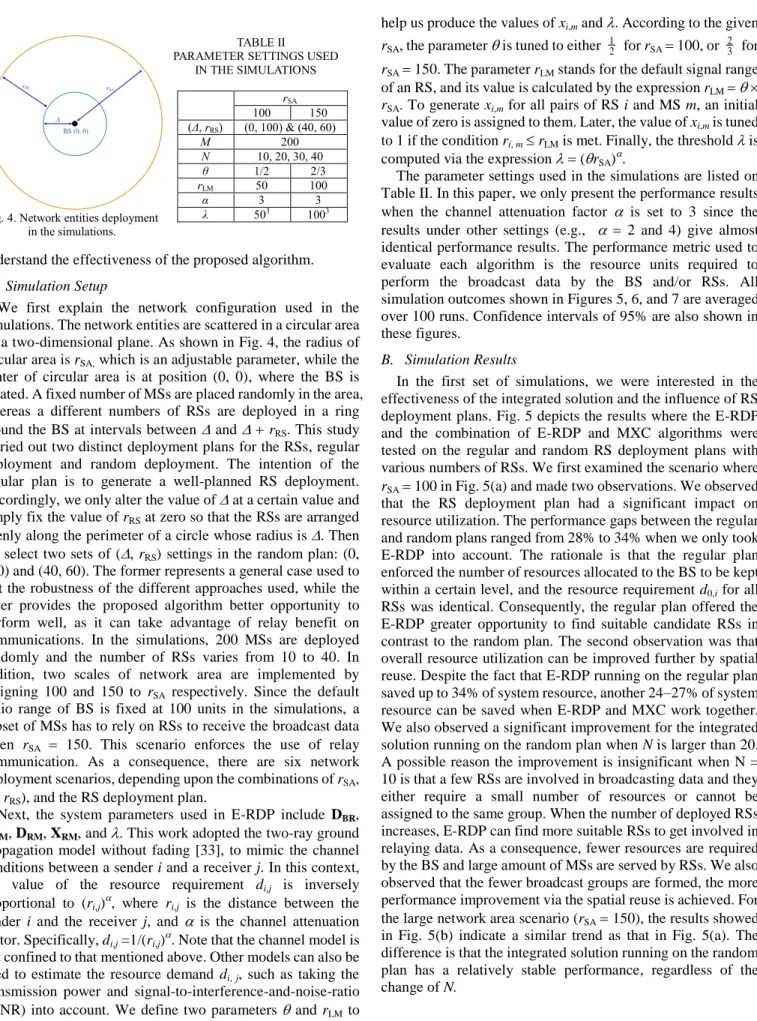
We first explain the network configuration used in the simulations. The network entities are scattered in a circular area on a two-dimensional plane. As shown in Fig. 4, the radius of circular area is rSA, which is an adjustable parameter, while the center of circular area is at position (0, 0), where the BS is located. A fixed number of MSs are placed randomly in the area, whereas a different numbers of RSs are deployed in a ring around the BS at intervals between and rRS. This study carried out two distinct deployment plans for the RSs, regular deployment and random deployment. The intention of the regular plan is to generate a well-planned RS deployment.
Accordingly, we only alter the value of at a certain value and simply fix the value of rRS at zero so that the RSs are arranged evenly along the perimeter of a circle whose radius is . Then we select two sets of (, rRS) settings in the random plan: (0, 100) and (40, 60). The former represents a general case used to test the robustness of the different approaches used, while the latter provides the proposed algorithm better opportunity to perform well, as it can take advantage of relay benefit on communications. In the simulations, 200 MSs are deployed randomly and the number of RSs varies from 10 to 40. In addition, two scales of network area are implemented by assigning 100 and 150 to rSA respectively. Since the default radio range of BS is fixed at 100 units in the simulations, a subset of MSs has to rely on RSs to receive the broadcast data when rSA 150. This scenario enforces the use of relay communication. As a consequence, there are six network deployment scenarios, depending upon the combinations of rSA, (, rRS), and the RS deployment plan.
Next, the system parameters used in E-RDP include DBR, DBM, DRM, XRM, and . This work adopted the two-ray ground propagation model without fading [33], to mimic the channel conditions between a sender i and a receiver j. In this context, the value of the resource requirement di,j is inversely proportional to (ri,j), where ri,j is the distance between the sender i and the receiver j, and is the channel attenuation factor. Specifically, di,j =1/(ri,j). Note that the channel model is not confined to that mentioned above. Other models can also be used to estimate the resource demand di, j, such as taking the transmission power and signal-to-interference-and-noise-ratio (SINR) into account. We define two parameters and rLM to
help us produce the values of xi,m and . According to the given rSA, the parameter is tuned to either 21 for rSA 100, or 32 for rSA 150. The parameter rLM stands for the default signal range of an RS, and its value is calculated by the expression rLM rSA. To generate xi,m for all pairs of RS i and MS m, an initial value of zero is assigned to them. Later, the value of xi,m is tuned to 1 if the condition ri, m rLM is met. Finally, the threshold is computed via the expression (rSA).
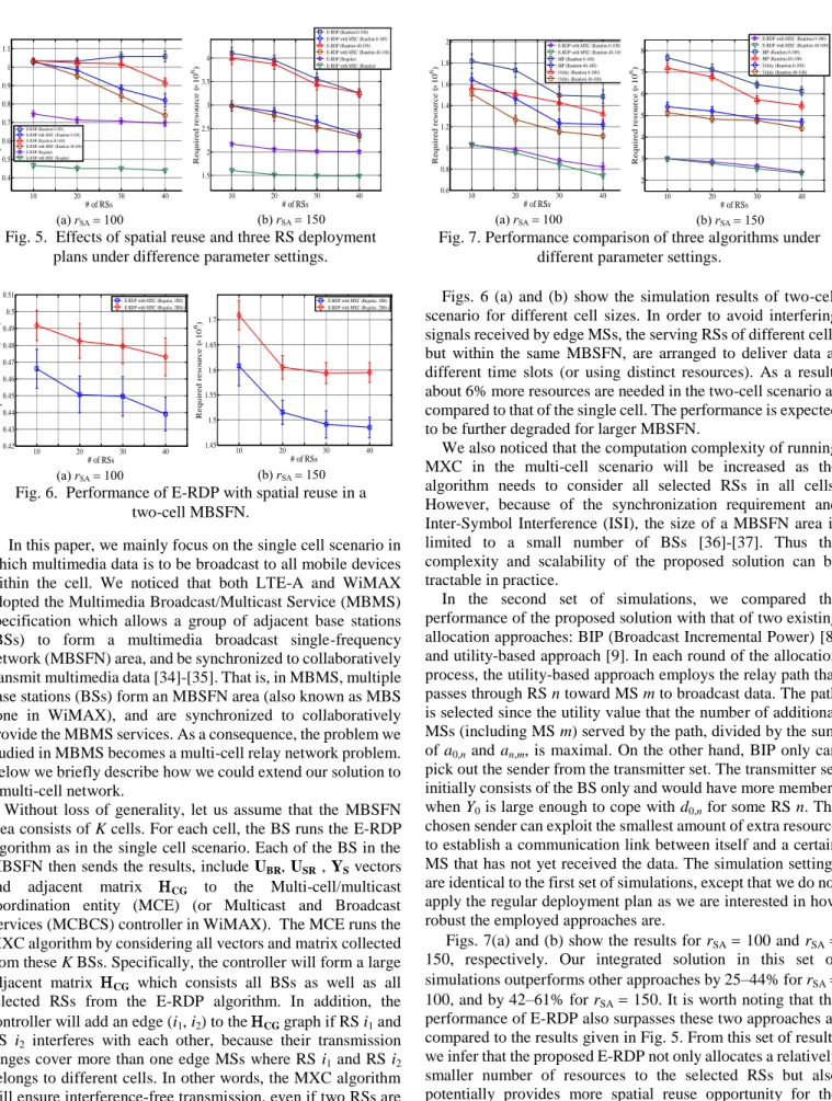
The parameter settings used in the simulations are listed on Table II. In this paper, we only present the performance results when the channel attenuation factor is set to 3 since the results under other settings (e.g., 2 and 4) give almost identical performance results. The performance metric used to evaluate each algorithm is the resource units required to perform the broadcast data by the BS and/or RSs. All simulation outcomes shown in Figures 5, 6, and 7 are averaged over 100 runs. Confidence intervals of 95% are also shown in these figures.
B. Simulation Results
In the first set of simulations, we were interested in the effectiveness of the integrated solution and the influence of RS deployment plans. Fig. 5 depicts the results where the E-RDP and the combination of E-RDP and MXC algorithms were tested on the regular and random RS deployment plans with various numbers of RSs. We first examined the scenario where rSA 100 in Fig. 5(a) and made two observations. We observed that the RS deployment plan had a significant impact on resource utilization. The performance gaps between the regular and random plans ranged from 28% to 34% when we only took E-RDP into account. The rationale is that the regular plan enforced the number of resources allocated to the BS to be kept within a certain level, and the resource requirement d0,i for all RSs was identical. Consequently, the regular plan offered the E-RDP greater opportunity to find suitable candidate RSs in contrast to the random plan. The second observation was that overall resource utilization can be improved further by spatial reuse. Despite the fact that E-RDP running on the regular plan saved up to 34% of system resource, another 24–27% of system resource can be saved when E-RDP and MXC work together.
We also observed a significant improvement for the integrated solution running on the random plan when N is larger than 20.
A possible reason the improvement is insignificant when N = 10 is that a few RSs are involved in broadcasting data and they either require a small number of resources or cannot be assigned to the same group. When the number of deployed RSs increases, E-RDP can find more suitable RSs to get involved in relaying data. As a consequence, fewer resources are required by the BS and large amount of MSs are served by RSs. We also observed that the fewer broadcast groups are formed, the more performance improvement via the spatial reuse is achieved. For the large network area scenario (rSA 150), the results showed in Fig. 5(b) indicate a similar trend as that in Fig. 5(a). The difference is that the integrated solution running on the random plan has a relatively stable performance, regardless of the change of N.
Fig. 4. Network entities deployment in the simulations.
TABLE II
PARAMETER SETTINGS USED IN THE SIMULATIONS
rSA
100 150
(Δ, rRS) (0, 100) & (40, 60)
M 200
N 10, 20, 30, 40
θ 1/2 2/3
rLM 50 100
α 3 3
λ 503 1003
BS (0, 0)
rSA
rRS

![Fig. 3. The flow chart of MXC approximation algorithm [7].](https://thumb-ap.123doks.com/thumbv2/9libinfo/9651057.674414/6.918.88.850.92.1045/fig-flow-chart-mxc-approximation-algorithm.webp)