Chapter 4
Transmission of Various Mode-Locked Laser with dispersion compensated fiber
Through the completed theoretical and experimental analysis of amplitude and phase modulated mode-locked figure eight fiber laser as shown in Chapter 2 and Chapter 3, in this chapter, we try to compare the performance of amplitude and phase modulated mode-locked laser system in Chapter 2 and Chapter 3. The content of this Chapter is organized as follows: Section 4-1 introduces the key issues of optical transmission system. Our system structure is discussed in Section 4-2. The theoretical models of our system are presented in Section 4-3. In Section 4-4, we discuss the simulation results and summary.
4-1 Introduction
High repetition rate pulse sources are essential for upgrading current optical telecommunication systems and have received significant attention in the past few years. The transmission capacity is determined by the bit rate per channel and the channel numbers. One channel of the bit rate of 2.5Gb/s is the great ripe state in Taiwan. The bit rate of 10Gb/s per channel
techniques are also becoming increasingly important for handling ultrashort pulse trains for high speed signal processing and for investigating the ultimate transmission capability of a single channel[107].
The effects of high speed transmission quality at shorter pulsewidths, the pulses spread more rapidly, and the dispersion becomes dominant.
High-bit-rate transmission is mainly limited by the single-channel effect of self-phase modulation[108].
It is commonly agreed that high-bit-rate communication systems have to be implemented in fiber-based networks. Long-distance transmission lines are essentially limited by the dispersion-induced broadening of the picosecond pulses used. This broadening depends on the dispersion parameter which is anomalous at l.55 μm and amounts to either β′′≈20 ps2/km(standard single mode fiber) or β′′≈1 ps2/km (dispersion-shifted fiber) [109]. One can either prevent or compensate for that broadening. The former option makes use of nonlinear effects in increasing the signal power and generating solitons[110]. The latter relies on linear dispersion management and currently attracts much interest in system design. One very promising opportunity exists in the periodic alignment of fiber pieces with opposite group velocity dispersion(GVD)[111]. First, the standard or dispersion-shifted fiber piece should have a length that coincides with the amplifier spacing, and second, the dispersion compensating fiber should have a fairly large dispersion to compensate for the acquired group delay in a short fiber piece. Normally, a fibre span consists of two fibre segments, one with positive dispersion and one with negative dispersion. The
dispersion and the relative position of these fibre segments need to be optimised, and this optimisation has been studied extensively for various span configurations and bit rates [112]. Both of the dispersion of SMF and non-zero dispersion-shifted fiber (NZDSF) can be completely compensated by some commercial dispersion-compensating fibre (DCF).
4-2 Single Channel Fiber Transmission System
We want to demonstrate our designed mode-locked laser the feasibility in practical application. We design two fiber transmission systems include:
unrepeatered and dispersion-managed system.
4-2-1 Unrepeatered Transmission System
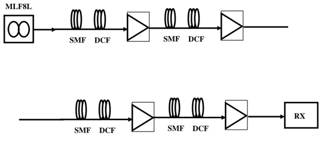
We use the mode-locked laser to transmit the data rate of 10 Gb/s, 20 Gb/s, 40Gb/s, and 50 Gb/s in unrepeatered transmission system. In Fig. 4-1, we set the mode-locked figure eight fiber laser(MLF8L) linking the long-distance single mode fiber(SMF), with an erbium-doped fiber amplifier(EDFA) to compensate the loss in SMF, and dispersion-compensating fibre (DCF) to compensate the dispersion. The attenuation, GVD, dispersion slope, and nonlinear coefficient of SMF are set 0.2 dB/km, 16 ps/nm.km, 0.08 ps/nm2.km, and 3 x 10-20 m2/W,
4-2-2 Dispersion-Managed Transmission System
In order to achieve the longest transmission distance, compensation in the fitting distance is necessary. Dispersion management in its simplest form consists of the concatenation of two alternate-sign dispersion sections that on average reduces the dispersion experienced by a propagating pulse[82]. Our designed system is to use DCF to compensate the dispersion, and use EDFA to amplify the signal as shown in Fig. 4-2. The SMF of 50 km use a DCF to compensate the chromatic dispersion. Then, connect an EDFA to amplify signal. With the system, the transmission distance can efficiently increase.
4-3 Theoretical Analysis of The System
In this Section, we propose the theoretical model of power penalty to analyze the transmission qualities.
4-3-1 Power Penalty Induced by Dispersion
Dispersion-induced pulse broadening affects the receiver performance.
The power penalty is defined as[113]
b D =10log f
δ (4-1)
where the fb is the pulse broadening factor. We derive the pulse broadening by time-domain ABCD matrix[90]. First, the pulse goes through SMF. The ABCD matrix can express as
( )
2 1
1 2
2 0 1 1 2
2 0
0 1 1
2 0 1 1 2 0
0 0 1 1
1 1 0
0 1
1 1
1 1
1 1
1 )
( 1
τ τ
β τ
β
τ β τ
β β
iC L
C L
C L C i L
L q i
q L
q
= +
⎟⎟⎠
⎜⎜ ⎞
⎝ +⎛ ′′
⎟⎟⎠
⎜⎜ ⎞
⎝
⎛ ′′
+
⎟⎟
⎠
⎞
⎜⎜
⎝
⎛ ′′
⎟⎟ +
⎠
⎜⎜ ⎞
⎝
⎛ ′′
+ +
=
− ′′
+
=
(4-2)
where the β1′′ is second-order dispersion of SMF, L1 is the length of SMF, is the initial pulsewidth, and C
τ0 0 is the initial chirp parameter. Thus, the pulsewidth and chirp parameter of going through SMF represent as
2 / 2 1
2 0 1 1 2
2 0
0 1 2 1
0
1 1
⎪⎭
⎪⎬
⎫
⎪⎩
⎪⎨
⎧
⎥⎥
⎦
⎤
⎢⎢
⎣
⎡
⎟⎟⎠
⎜⎜ ⎞
⎝ +⎛ ′′
⎟⎟⎠
⎜⎜ ⎞
⎝
⎛ ′′
+
= τ
β τ
τ β
τ LC L (4-3)
2
2 0 1 1 2
2 0
0 1 1
4 0 1 1 2
0 0 2
0 0 1 1
2 1 1
1 1
⎟⎟⎠
⎜⎜ ⎞
⎝ +⎛ ′′
⎟⎟⎠
⎜⎜ ⎞
⎝
⎛ ′′
+
⎟⎟
⎠
⎞
⎜⎜
⎝
⎛ ′′
⎟⎟ +
⎠
⎜⎜ ⎞
⎝
⎛ ′′
+
=
τ β τ
β
τ β τ
τ β τ
L C
L
L C
C L C
(4-4)
Then, the broadening pulse is compensated by DCF. The ABCD matrix of DCF expresses in Eq (4-5):
⎟⎟
⎟
⎠
⎞
⎜⎜
⎜
⎝
⎛ − ′′
⎟⎟=
⎠
⎜⎜ ⎞
⎝
⎛ − ′′
⎟⎟
⎟
⎠
⎞
⎜⎜
⎜
⎝
⎛
1 0
1 1 1
0 1 1 0
1 12 2 2 2 i 2L2
L B
BG iβ G β
(4-5)
where BG is the bandwidth of DCF, β2′′ is the second-order dispersion, and L2 is the length of DCF. Thus, the pulsewidth and chirp parameter of experiencing DCF can derive by
2 2
2
2 2 2
2 1
1 2 1
1
2 2 2
1
1 1
1 1 1
1
1 1 1
1
β τ τ
τ β
iC L
B i iC
iC
L B i
q
q
G G
= +
⎟⎟⎠
⎜⎜ ⎞
⎝
⎛ − ′′
+ +
+
=
⎟⎟⎠
⎜⎜ ⎞
⎝
⎛ − ′′
+ (4-6)
( )
1/21 2 2 2 1
2 ⎟⎟
⎠
⎞
⎜⎜
⎝
⎛
+
= +
y C x
y τ x
τ (4-7)
(
2 1 2)
2
1 2
2 x y
y C xC
+
⎟⎟ −
⎠
⎜⎜ ⎞
⎝
= ⎛ τ τ
(4-8)
where
2 1
1 2 2 2
1 2
1 1
τ β τ
C L
x w ′′
Δ + +
= (4-9)
2 1
2 2 2
1 2
1
τ β τ
L w
y C ′′
Δ −
= (4-10)
Thus, we find the broadening factor
0 2
τ
= τ
fb . The power penalty induced by dispersion is known.
4-4 Simulated model of The System
In this Section, we propose the simulated Gaussian approximation model of bit error rate(BER) to analyze the transmission qualities.
4-4-1 Bit Error Rate
In this Section, we try to set the theoretical model of our designed unrepeatered transmission system. We consider the several impact factors of the system include: the noises induced by EDFA, thermal noise, shot noise, power of change caused by dispersion, and RMS jitter.
We first define the parameter Q represents as[114]
0 1
0
1 σ
σ +
= I −I
Q (4-11)
where the I1 and I0 are the electrical signal current for “mark” and “space”, respectively. The σ1 and σ0 are the total noise current.
The thermal noise power σT2 and shot noise power σS2 represent as
(
kTemp RL)
NF fT2 = 4 / ⋅ ⋅Δ
σ (4-12)
hv f GP
e a
S
= η Δ
σ2 2 2 (4-13)
hv n
G
SASE = ( −1) spχ (4-14)
In the above equations, SASE is the spontaneous power density, the k is
Boltzmann’s constant, is the absolute temperature, is the load resistance, NF is the amplifier noise figure,
Temp RL
Δf is received noise
bandwidth, q is the electric charge, ℜ is the detector responsivity, is the signal power into amplifier, is spontaneous-emission factor, the parameter
Pa
nsp
χ is the nonuniform carrier density distribution due to gain saturation, and h is Plank’s constant.
In addition, there are noise terms due to EDFA amplified spontaneous emission(ASE) and its interaction with the signal. The signal-ASE beat noise power due to signal and ASE noise interaction, the noise power due to ASE alone. They represent by[115-117]
NF f eGBG
ASE
ASE− =η Δ ⋅
σ2 (4-15)
NF f GB
e G
shot
ASE− = η Δ ⋅
σ2 2 2 (4-16)
hv
NF f P G
e a
ASE sig
⋅
= Δ
−
2 2 2
2 2 η
σ (4-17)
where the BBG is bandwidth of DCF. The timing jitter is also a key impact factor to limit the transmission distance. The RMS jitter can represent as[84]
( )
[
0 2]
0 2
2 N N N d d C
E S
f A
A A
m sp
j = τ + + +
τ (4-18)
where the Ssp is the accumulated power spectral density, 2 0 0
) 1
( C
m = +τ
τ
is the minimum pulsewidth occurs when the pulsewidth is unchirped,
0 0
0 πPτ
E = is the input pulse energy, P0 is input pulse power, NA is the number of amplifier, d = β ′′LA /τm2 for the amplifier distance LA and average dispersion β ′′, and for a postcompensation element of length L
/ m2 G G
f L
d = β′′ τ
G and dispersion β ′′. The current fluctuation and noise induced by RMS jitter represent by[76]
( )
a j Rxt ⎟⎟ R ℜP
⎠
⎜⎜ ⎞
⎝
⎛ −
= 2 8 2
3
2 4π τ
σ (4-19)
( )
a j Rxj R P
i ⎟⎟⎠ ℜ
⎜⎜ ⎞
⎝
⎛ −
=
Δ 2 8 2
3
4π τ
(4-20)
where the σt is the RMS value of the current fluctuation induced by timing jitter, is the average value of current fluctuation, and R
ij
Δ
a is data rate.
Because the fiber has larger dispersion in 1.5 μm, the intersymbol interference(ISI) generally much larger than other noises, it is the
dominating term and is close to the actual BER. The noise induced by ISI can be expressed as[116-120]
2
0
2 / 1
0 2
2 2 4
2
⎪⎪
⎭
⎪⎪
⎬
⎫
⎪⎪
⎩
⎪⎪
⎨
⎧
− +
⎥⎦
⎢ ⎤
⎣
⎡ ⎟⎟⎠
⎜⎜ ⎞
⎝
⎛ +
− ℜ
=
f r
f r Rx
b H
P q
f τ τ
τ
τ τ τ
σ (4-21)
2
0
2 / 1
2
2 2 2
⎪⎪
⎭
⎪⎪
⎬
⎫
⎪⎪
⎩
⎪⎪
⎨
⎧
− +
⎥⎦
⎢ ⎤
⎣
⎡ +
ℜ
=
f r
f r Rx b
L
P q
f τ τ
τ
τ τ
σ (4-22)
where and are signal dependent noise power when bit “1” and bit
“0”, respectively. The
2
σH σL2
τ0 is the initial pulse width, the τr is rise time, and the τf is the falling time. Thus, the worst case of BER can be defined by
) 2 / 2 (
1 8 ) 1 2 / 2 (
1 8 1
L
H erfc Q
Q erfc
BER = × + × (4-23)
The QH represents as
0 1
1
σ σ +
Δ
= −
H j H
i
Q I (4-24)
where
(
2 2 2 2 2 2 2)
2
1H σT σS σASE ASE σASE shot σsig ASE σt σH
σ = + + − + − + − + +
(
2 2)
2
0 = σT +σASE−ASE
σ
The QL represents as
0 1
1
σ σ +
Δ
= −
L j L
i
Q I (4-25)
where
(
2 2 2 2 2 2 2)
2
1L σT σS σASE ASE σASE shot σsig ASE σt σL
σ = + + − + − + − + +
(
2 2)
2
0 = σT +σASE−ASE
σ
4-5 Numerical Results
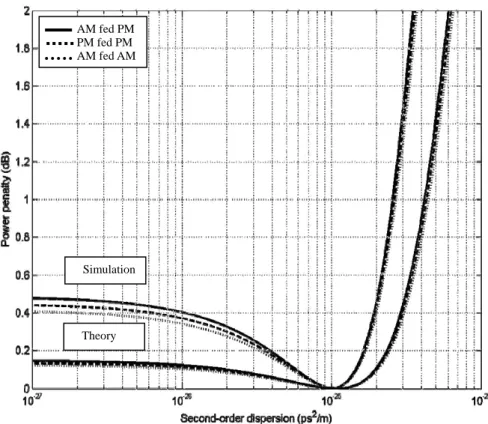
Fig. 4-3 comparing the dispersion induced power penalty vs. the second order dispersion of postcompensting DCF with various mode-locked method, which including AM signal fed amplitude modulator to excited short pulse, AM signal fed phase modulator to excited short short and PM signal fed phase modulator to excited short pulse. The optimal power penalty is 0. Using the DCF to compensate the dispersion can reduce the dispersion induced power penalty to improve the performance. We can find the optimal second-order dispersion of DCF is 1.2 x 10⁻²⁵ in Fig. 4-3.
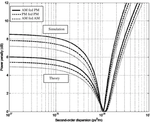
With observing the power penalty, we can find the optimum values of dispersion compensation are 1.1x 10⁻²⁵, 1.06 x 10⁻²⁵, and 0.97 x 10⁻²⁵ as shown in Fig. 4-4, Fig. 4-5, and Fig. 4-6, respectively. The compensation values of DCF are decided by initial pulsewidth, accumulated chirp parameters. Besides, comparing with the theory and simulation result in Fig.
4-3 to Fig. 4-6, the dispersion compensation is more important in high data rate than low data rate. The not enough second-order dispersion causes the power penalty, but the too large second-order dispersion of postcompensating DCF also causes the high power penalty. We also can find the difference between the theory and simulation with the same pulsewidth of various mode-locked method is below 1 dB. The theory and simulation value is very closed in Fig. 4-6.
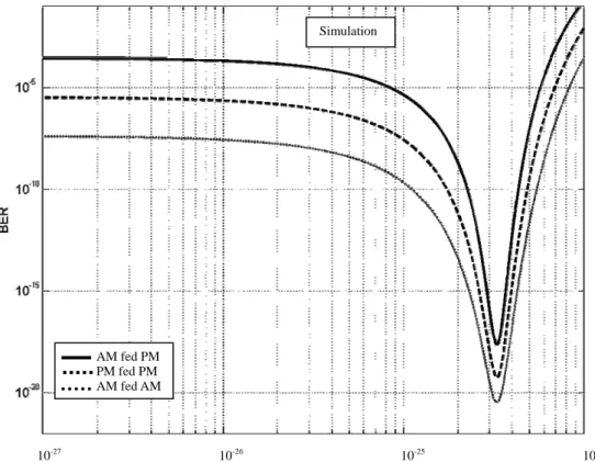
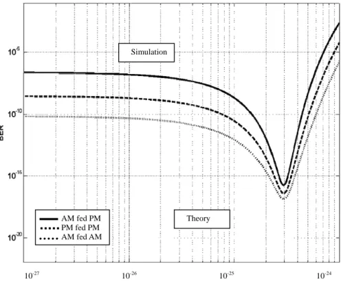
Fig. 4-7 depicts the BER vs. second-order dispersion of DCF with various mode-locked method. Because of the ISI, we find the effect of dispersion compensation dominate the system performance. We can find the optimal second-order dispersion of DCF is 5.2 x 10⁻²⁴ in Fig. 4-7. With
compensation are 5.3x 10⁻²⁴, 5.4. x 10-24, and 5.5 x 10⁻²⁴ as shown in Fig.
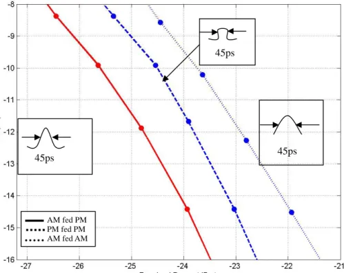
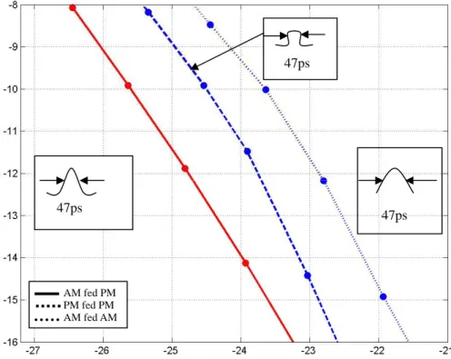
4-8, Fig. 4-9, and Fig. 4-10, respectively. The compensation values of DCF are decided by initial pulsewidth, accumulated chirp parameters. Besides, comparing with the theory and simulation result in Fig. 4-7 to Fig. 4-10 the dispersion compensation is more important in high data rate than low data rate. The not enough second-order dispersion causes the BER, but the too large second-order dispersion of postcompensating DCF also causes the high BER. After Fig. 4-11, we do simulation with software of OptiSystem in dispersion-managed system, the data rate and pulsewidth are serious to affect the performance. In Fig. 4-11, Fig. 4-12 and Fig. 4-13, we depicts the BER vs. the received power with various pulse shape of repetition rate 10b/s, we depicts the puleswidth 45ps with various mode locked laser in Fig. 4-11, the Fig. 4-12 and Fig. 4-13 depict the BER vs. the received power of various mode locked laser with pulsewidth 46ps and 47ps, respectively. In Fig. 4-14, Fig. 4-15 and Fig. 4-16, we depict the BER vs.
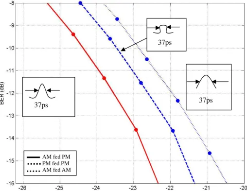
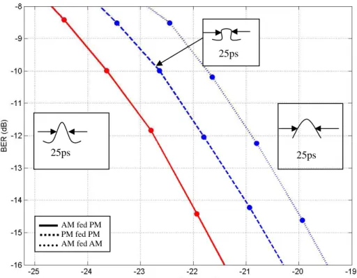
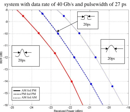
the received power with various pulse shape of repetition rate 20b/s, we depicts the puleswidth 35ps with various mode locked laser in Fig. 4-14, the Fig. 4-15 and Fig. 4-16 depict the BER vs. the received power of various mode locked laser with pulsewidth 36ps and 37ps, respectively. In Fig. 4-17, Fig. 4-18 and Fig. 4-19, we depict the BER vs. the received power with various pulse shape of repetition rate 40b/s, we depicts the puleswidth 25ps with various mode locked laser in Fig. 4-17, the Fig. 4-18 and Fig. 4-19 depict the BER vs. the received power of various mode locked laser with pulsewidth 26ps and 27ps, respectively.in Fig. 4-20, Fig.
4-21 and Fig. 4-22, we depict the BER vs. the received power with various
pulse shape of repetition rate 50b/s, we depicts the puleswidth 20 ps with various mode locked laser in Fig. 4-20, the Fig. 4-21 and Fig. 4-22 depict the BER vs. the received power of various mode locked laser with pulsewidth 21ps and 22 ps, respectively. From Fig. 4-11 to Fig. 4-22, we can find the AM fed amplitude modulator transmission system is better performance than the other transmission system in the BER vs. the received power.
4-6 Distance Analysis
If we use the unrepeatered transmission system. In AM fed amplitude modulator transmission system, we can ensure the data rate of 10 Gb/s, 20 Gb/s, 40 Gb/s, and 50 Gb/s can transmit 50 km, 40 km, 35 km, and 30 km, respectively.In AM fed phase modulator transmission system, we can ensure the data rate of 10 Gb/s, 20 Gb/s, 40 Gb/s, and 50 Gb/s can transmit 40 km, 30 km, 30 km, and 25 km, respectively.In FM fed phase modulator transmission system, we can ensure the data rate of 10 Gb/s, 20 Gb/s, 40 Gb/s, and 50 Gb/s can transmit 45 km, 40 km, 35 km, and 30 km, respectively.
If we use the dispersion-managed transmission system, the transmission
transmission system, the data rate of 10 Gb/s can transmit 150 km use the dispersion of DCF. As mentioned early, we know the system has little change of power penalty even the DCF tuning large dispersion value in data rate of 20 Gb/s can transmit 135 km and achieve 10-15 at dispersion of DCF of –80 ps/nm. The transmission distance can reach 110 km with data rate of 40 Gb/s. The transmission can reach 105 km with data rate of 50 Gb/s. In AM fed phase modulator transmission system, the data rate of 10 Gb/s can transmit 120 km use the dispersion of DCF. As mentioned early, we know the system has little change of power penalty even the DCF tuning large dispersion value in data rate of 20 Gb/s can transmit 110 km and achieve 10-15 at dispersion of DCF of –80 ps/nm. The transmission distance can reach 105 km with data rate of 40 Gb/s. The transmission can reach 100 km with data rate of 50 Gb/s.
In FM fed phase modulator transmission system, the data rate of 10 Gb/s can transmit 135 km use the dispersion of DCF. As mentioned early, we know the system has little change of power penalty even the DCF tuning large dispersion value in data rate of 20 Gb/s can transmit 120 km and achieve 10-15 at dispersion of DCF of –80 ps/nm. The transmission distance can reach 105 km with data rate of 40 Gb/s. The transmission can reach 100 km with data rate of 50 Gb/s.
4-7 Summary and Discussion
We can analyzer eye pattern in Fig. 4-23, Fig. 4-24, Fig. 4-25, and Fig.
4-26, respectively. The eye pattern with 50GHz pulse before transmitted by 100km fiber in Fig. 4-23. In Fig. 4-24, we find the eye pattern is compressed vertically, so we know the SNR of the transmission system has been reduced. In Fig. 4-25, we find the eye pattern is compressed vertically and horizontally at the same time, so we know the Timing error of the transmission system has been worse. In Fig. 4-26, we find the eye pattern is compressed horizontally, so we know the Phase distortion of the transmission system has beenreduced.
MLF8L
Rx
SMF DCF
Fig. 4-1 The unrepeatered transmission system with various data rate and pulse shape. MLF8L: mode-locked figure eight laser, SMF: single mode fiber, DCF: dispersion compensating fiber
MLF8L
RX DCF
SMF SMF DCF
SMF DCF SMF DCF
Fig. 4-2 The dispersion-managed transmission system with various data rate and pulse shape.
Fig. 4-3 Comparing the power penalty of data rate of 10 Gb/s and pulsewidth 45ps with various mode locked method
Simulation
Theory Simulation
Theory
AM fed PM PM fed PM
AM fed AM
AM fed PM PM fed PM
AM fed AM
Fig. 4-5 Comparing the power penalty of data rate of 40 Gb/s and pulsewidth
Simulation
Theory
25 ps with various mode locked method
AM fed PM PM fed PM AM fed AM
Fig. 4-6 Comparing the power penalty of data rate of 50 Gb/s and pulsewidth 20 ps with various mode locked method
Simulation
Theory
AM fed PM PM fed PM
AM fed AM
Simulation
AM fed PM PM fed PM
AM fed AM
mode locked method
Fig. 4-7 Comparing the BER of data rate of 10 Gb/s and pulsewidth 45ps with various
10-27 10-26 10-25 10-24
Simulation
AM fed PM PM fed PM
AM fed AM
10-27 10-26 10-25 10-24
Simulation
AM fed PM PM fed PM
AM fed AM
Theory
10-27 10-26 10-25 10-24 Second-order dispersion (ps2/m)
10-27 10-26 10-25 10-24
Second-order dispersion (ps2/m) Theory
AM fed PM PM fed PM
AM fed AM
Simulation
Fig. 4-9 Comparing pulsewidth 25ps with various
Fig. 4-10 Compar and pulsewidth 45ps with various
the BER of data rate of 40 Gb/s and mode locked method
ing the BER of data rate of 50 Gb/s mode locked method
45ps
45ps 45ps
AM fed PM PM fed PM
AM fed AM
Fig. 4-11 The BER vs. the received power in dispersion-managed transmission system with data rate of 10 Gb/s and pulsewidth of 45ps
46ps
46ps 46ps
AM fed PM PM fed PM
AM fed AM
47ps
47ps 47ps
AM fed PM PM fed PM
AM fed AM
Fig. 4-13 The BER vs. the received power in dispersion-managed transmission system with data rate of 10 Gb/s and pulsewidth 47ps
35ps
35ps 35ps
AM fed PM PM fed PM
AM fed AM
Fig. 4-14 The BER vs. the received power in dispersion-managed transmission system with data rate of 20 Gb/s and pulsewidth transmission 35ps
36ps
36ps 36ps
AM fed PM PM fed PM
AM fed AM
Fig. 4-15 The BER vs. the received power in dispersion-managed transmission system with data rate of 20 Gb/s and pulsewidth of 36ps
37ps
37ps 37ps
AM fed PM PM fed PM
AM fed AM
Fig. 4-16 The BER vs. the received power in dispersion-managed transmission
25ps
25ps 25ps
AM fed PM PM fed PM
AM fed AM
Fig. 4-17 The BER vs. the received power in dispersion-managed transmission system with data rate of 40 Gb/s and pulsewidth 25 ps
26ps
26ps 26ps
AM fed PM PM fed PM
AM fed AM
Fig. 4-18 The BER vs. the received power in dispersion-managed transmission system with data rate of 40 Gb/s and pulsewidth 26 ps
27ps
27ps
27ps
AM fed PM PM fed PM
AM fed AM
Fig. 4-19 The BER vs. the received power in dispersion-managed transmission system with data rate of 40 Gb/s and pulsewidth of 27 ps
20ps
20ps 20ps
AM fed PM PM fed PM
AM fed AM
Fig. 4-20 The BER vs. the received power in dispersion-managed transmission
21ps
21ps 21ps
AM fed PM PM fed PM
AM fed AM
Fig. 4-21 The BER vs. the received power in dispersion-managed transmission system with data rate of 50 Gb/s and pulsewidth of 21 ps
22ps
22ps
22ps
AM fed PM PM fed PM
AM fed AM
Fig. 4-22 The BER vs. the received power in dispersion-managed transmission system with data rate of 50 Gb/s and pulsewidth 22 ps
Fig.4-23 The eye pattern with 50GHz pulse before transmitted by 100km
10-6 Signal (V) Signal (V)
10-12
10-12 10-6
Time(s)
Time(s)
0 10 20 30 40 50 60 70 80 4
2 8
6 10
0 10 20 30 40 50 60 70 80 2
6
4 8 10
Fig.4-24 The eye pattern with 50GHz pulse after transmitted by 100km
10-6
10-12 2
6
4 8 10
0 10 20 30 40 50 60 70 80
Signal (V)
Time(s)
Fig.4-25 The eye pattern with 50GHz pulse after transmitted by 100km in AM fed phase modulator transmission system
10-12 Time(s)
10-6
2 4 6 8 10
0 10 20 30 40 50 60 70 80
Signal (V)
Fig.4-26 The eye pattern with 50GHz pulse after transmitted by 100km in PM fed phase modulator transmission system