高低技術勞工間所得不均與休閒不均

國立臺灣大學社會科學院經濟學系 碩士論文

Department of Economics College of Social Science National Taiwan University

Master Thesis

高低技術勞工間所得不均與休閒不均

Wage Inequality and Leisure Inequality between High-Skilled Agents and Low-Skilled Agents

詹禮謙 Li-Chien Chan

指導教授：蔡宜展博士、吳亨德博士

Advisor: Yi-Chan Tsai, Ph.D. and Hendrik Rommeswinkel, Ph.D.

中華民國 108 年 8 月 August 2019

Acknowledgement

I am thankful for everything that leads me to explore my research wisdom. Especially, I appreciate my advisers, Professor Tsai and Professor Hendrik. They give me helpful comments on my work. Professor Tsai usually asks precise questions whenever we discuss our paper.

I learned a lot from his questions and began to know how to do research independently. Professor Hendrik often provides me with mathematics comments. That influences how I construct a meaningful economic model from mathematics view. Furthermore, although my eyes hindered me in my efforts to finish the paper, I am grateful to people who help me to accomplish this paper.

In particular, I would like to thank the faculty members,

Miss Chung in disability center, Miss Li in economics

office, and Ms Chen in mathematics department, for

helping me connect students who are willing to assist

me in completing the paper. Moreover, Professor Tsai

provides me financial support to affirm of my work and

Professor Hendrik usually helps me to cross a road

whenever we meet at crossroads. All of above

encourage me to do my best on my work. I will keep

work no matter what the end is. Thanks for everything I

met. If there is any error idiocy and any inconsistency,

these remain my own.

中文摘要

本篇論文的理論模型延續 [1] 的模型，進一步將勞動與休閒選擇的 設定納入模型內，進而解釋近幾十年來，高低技術勞工間所得與休閒 不均的現象。在我們的理論模型中，高低技術勞工將單位時間分配於 休閒與勞動，其在提供勞動力的同時，必須運用知識解決生產過程中 所遇到的問題，而從生產過程中，所獲得的所得，用於其消費。在市 場均衡的條件下，我們進行比較靜態分析，發現：溝通技術水準的改 善，是導致高低技術勞工間休閒不均的原因；同時，此種技術的改善，

也是導致兩者所得不均的原因。

Wage Inequality and Leisure Inequality between High-Skilled Agents and

Low-Skilled Agents

Li-Chien Chan

Contents

1 Introduction 4

2 Model 7

3 Equilibrium 14

4 Simulation and Results 18

5 Conclusion and References 26

Abstract

This paper constructs an equilibrium theory to explain wage inequality and leisure inequality between high-skilled agents and low-skilled agents. Following [1], our theory ex- tends their theory to consider labor-leisure choice. This ex- tension allows us to explore leisure inequality between high- and low-skilled agents in a knowledge economy. In our econ- omy, knowledge is a necessary input in production and agents allocate their time on leisure and labor. An equilibrium al- location is determined by the optimal choices of agents that use knowledge to produce and consume a single good. Our main results show that both wage inequality and leisure in- equality between high-skilled agents and low-skilled agents are caused by improvements in communication technology.

Wage inequality is amplified by leisure inequality, leading to a dramatic difference in earnings. These results are consis- tent with empirical findings.

1 Introduction

Wage inequality is the inequality of the wage distribution: the very top of it has increased dramatically, meanwhile the bottom of it has decreased sharply. This phenomenon has been widely discussed in many studies during the past few years. There are many perspective in these studies, in- cluding educational attainment, technological change, gender, and organi- zation changes. [3] stated that earning of college graduates have increased since 1979, while it has currently declined for high school graduates. For technological change, [4] asserted that due to the production technology shift from unskilled labor to skilled labor, skill premium increased. Later, [8] showed that there was a significantly increased in women’s earnings rel- ative to the men’s during late 1970s and 2005. For organization changes, [1] demonstrated that wage inequality between high-skilled agents and low-skilled agents in an organization is caused by the reduction in com- munication cost in the 1980s and the late 1990s. [5, 6] document that low-skilled individuals experienced a large increase in leisure time than high-skilled individuals did during 1965 to 2005. The trends in leisure are known as leisure inequality. This inequality seems to be the mirror image of wage inequality over those decades. However, in [1], the theoretical part of leisure inequality lacks discussion. Thus, our paper extends the theory in [1] by a labor-leisure foundation and demonstrates that improvements in communication technology leads to both wage inequality and leisure inequality between high-skilled agents and low-skilled agents.

Our model is best correspond to [1]. We therefore give an overview of the knowledge economy in [1]. This theory describes how agents organize production through a market mechanism. To produce, agents are required to solve problems. Solving problems requires knowledge. To obtain pro- duction knowledge, agents incur a learning cost. The learning cost is associated with the agents’ ability and information technology they use.

If the cost of using the information technology, such as cheaper database storage, is lower (The improvement in the technology), that is conducive to the knowledge acquisition. Given the information technology, an agent with higher ability encounters a lower learning cost than an agent en- dowed with lower ability does. If an agent has enough knowledge, he can

fully solve the problem and obtains one unit of output. Otherwise, an agent receives output equivalent to the fraction of the problem he solves, and sells the unsolved problems to the market. The price of the problem depends on its difficulty: more difficult problems in equilibrium have a higher price on the market as they may generate more output. Agents trade the unsolved problem with each other. A buyer, whose ability is higher than sellers, buys the problems from sellers. Communication tech- nology is the time cost used by her to understand about the problems she buys. The improvement in this technology leads to the wage inequality among skilled agents in their paper. The main difference between their model and ours is that we further consider labor-leisure choice under their framework.

In order to explore time allocation amont agents with different skills, we assume that all agents allocate their time on labor and leisure. His utility depends on his consumption and leisure time. For their work, agents with different abilities are required to obtain production knowledge at a cost and decide optimally how much knowledge they need to solve problems.

As in the literature we mentioned above, because agents are endowed with different abilities, acquiring production knowledge costs them differently.

That is, high-skilled agents have a relative advantage in knowledge acqui- sition.

There are two types of agents in our economy: workers and one man- ager. A worker, who has lower ability, draws one problem from a known probability distribution. The problem is solved if its difficulty is below his level of knowledge. Once the problem is solved, he obtains one unit of output. Otherwise, he receives a fraction of the output and sells the unsolved problem at a market price to the manager. A manager, whose ability is higher than the workers, buys the unsolved problems from the workers and then she communicates with workers about the problems at a time cost. Similar to the workers, if she can fully solve the problems, she obtains the outputs. She receives the fraction of the output from the problems she solves.

Agents use their income to consume a single good. Their choice of pro-

duction knowledge, consumption, and leisure is the solution to their utility maximization problem. Their optimal decisions determine the market- clearing conditions, including the problem market and the goods mar- ket. The economy-wide equilibrium is an allocation where agents acquire knowledge, consume a single good, and spend their time on leisure and labor.

Our theory displays two features consistent with empirical findings.

First, following [1], wage inequality between high-skilled agents and low- skilled agents is caused by improvements in communication technology.

Second, this improvement also leads to leisure inequality between high skill agents and low skill agents. By our theory, the explanation of the first finding is the decrease in the relative cost of solving problems. That is, the cost of knowledge acquisition is higher than the cost of seeking help from high-skilled agents, so lower-skilled agents tend to sell unsolved problems on the market rather than solving the problems by themselves. Further- more, we explain the second finding as follows: due to improvements in communication technology, low-skilled agents tend to spend more time on leisure than high-skilled agents do. That is, as the technology improves, low-skilled agents tend to work less and high-skilled agents tend to spend more time working. All of the above explanations are consistent with each other: due to the improvement, the decline in earnings implies the workers spend less time working, and thus spend more time on leisure than before. Similarly, since the technology has improved, the manager needs to solve a larger proportion of the unsolved problems. It implies she earns more and spends less time on leisure than before. Both of the above empirical findings can be found in [2, 5, 6, 9].

The paper is organized as follows: section 2 presents our model, section 3 describes the equilibrium conditions of our model, section 4 shows the results from our simulation, and section 5 concludes our framework.

2 Model

Agents in our economy maximizes their utility. Their utility depends on their consumption and leisure. They spend their time on leisure and la- bor. On the job, they learn how to solve problems at a cost. The learning cost is needed for them to acquire production knowledge. One unit of output is realized by solving one problem. The problem is solved by an agent who has enough knowledge. The agent who cannot completely solve the problem obtains a fraction of one unit of output and then sells it at a market price. On the market, agents are heterogeneous in skill. Each of them learns how to solve problems and trades the unsolved problems with each other. A seller, whose ability (skill) is lower than buyers, sells the unsolved problem at a price to the buyers. A buyer, whose role is to help the seller solve the unsolved problem, buys the problem from the seller and spends a fraction of her time to communicate (understand) with the seller about the unsolved problem. Through the market mechanism, problems can be solved efficiently by agents with different skills: The low-skilled agents solve relatively routine problems and the high-skilled agents solve harder ones. They work so they have their income and spend it on comsuming goods. Therefore, their optimal decisions on production knowledge, consumption, and leisure are the solution to the problem of how to maximize their utility.

Consider, now, there are two types of agents on the market: workers and problem-solvers. A worker with ability α_w draws one problem from problem distribution G(Z), where G⁰(Z) > 0, G⁰⁰(Z) < 0, and Z is the degree of difficulty of the problem. He can solve the problem by himself if he has enough production knowledge. He can use knowledge Z_w ∈ R^{+ to} solve an interval [0, Z] of the problem. To simplify the notation, a solved proportion of the problem G(Z_w) is defined as y_w = G(Z_w). The simpli- fication implies Z_w = Z(y_w), where Z(y_w) = G⁻¹(y_w), and so Z⁰(y_w) > 0 and Z⁰⁰(y_w) > 0. Z(y_w) means the knowledge required to solve a propor- tion y_w of the problem. For him, the cost of learning the knowledge to solve an interval [0, Z] of the problem is

(1) : c(α_w, i) · Z_w = c(α_w, i) · Z(y_w),

where α_w is his ability and i is the information technology he uses to acquire production knowledge. If the cost function C is affine, it satisfies supermodularity in ability α_w and knowledge Z_w, as required for com- parative advantage: A worker with higher ability α_w has a comparative advantage in problem-solving because he incurs a lower learning cost to acquire knowledge used in solving the problem than one with lower ability does. The partial derivative of the cost function with respect to Z_w is

(2) : ∂c(α_w, i)Z_w

∂Z_w = c(α,_w, i).

This derivative shows the cost of solving more difficult problems de- pends on the worker’s ability, α_w, and the technology he uses, i. The worker endowed with higher ability incurs lower learning cost when he is required to learn how to solve more difficult problems. That is, the mixed partial derivative of the cost function with respect to Z_w and α_w should be less than zero,

(3) : ∂²c(α_w, i)Z

∂Z_w · ∂α_w < 0.

Furthermore, i is the information technology used in knowledge ac- quisition such as database storage. The improvement in this technology decreases the cost of acquiring knowledge,

(4) : ∂²c(α_w, i)Z

∂Z_w∂i > 0.

Since a proportion of the problem y_w is a one-to-one function of the pro- duction knowledge Z_w, once y_w is determined, Z_w is determined. When

a worker uses Z_w to solve a problem, we can simplify it as he uses the knowledge Z(y_w) to solve the problem. If he can solve it, he receives one unit of output; otherwise, he obtains the return on solving a fraction of the problem y_w < 1 and sells the unsolved problem in the market at price p(y_w). His total income are from the revenue of selling the unsolved problem and the return on solving a fraction of the problem. He uses his income to consume a single good. Besides, a worker spends his time on labor and leisure. He spends t_w(y_w, α_w) units of time on problem-solving and l_w units of time on leisure. The function t_w(y_w, α_w) is increasing in problem difficulty y_w and decreasing in ability α_w. It implies more difficult problems require more time to solve and the worker with higher ability takes less time to solve problems than the one with lower ability does. A worker’s utility depends on his consumption and leisure, u(c_w, l_w).

Therefore, his problem is to maximize his utility by choosing production knowledge y_w, consumption c_w, and leisure l_w, given his time constraint and budget constraint.

Problem I: (A worker’s problem)

{c^∗_w, l^∗_w, y_w^∗} = arg max

cw,lw,yw

u(c_w, l_w) s.t.

Time constraint: 1 = l_w + t_w(y_w, α_w)

Budget constraint: c_w = y_w + p(y_w) · (1 − y_w) − c(α_w, i) · Z(y_w) The first-order conditions are given by

(5) : {l_w} : ∂u(c^∗_w, l_w^∗)

∂l_w = λ^∗_w (6) : {c_w} : ∂u(c^∗_w, l_w^∗)

∂c_w = µ^∗_w

(7) : {y_w} : 1 − p(y_w^∗) + (1 − y_w^∗)p⁰(y_w^∗) − c(α_w, i)Z⁰(y_w^∗)

∂t_w(y^∗_w, α_w)/∂y_w = λ^∗_w µ^∗_w (8) : {λ_w} : 1 = l^∗_w+ t_w(y_w^∗, α_w)

(9) : {µ_w} : c^∗_w = y_w^∗ + (1 − y^∗_w)p(y^∗_w) − c(α_w, i)Z(y_w^∗),

where λ_w and µ_w are the Lagrange multiplier.

Equation (5) and (6) show the marginal utility of consumption and leisure for a worker. To be clear, equation (5) means the marginal utility of a worker’s leisure is equal to the Lagrange multiplier λ_w. That is, λ_w is the shadow price of his leisure time because it assesses the marginal benefit of his leisure decision. Similarly, equation (6) means the marginal utility of a worker’s consumption is equal to the Lagrange multiplier µ_w. In other words, the Lagrange multiplier µ_w is the shadow price of his con- sumption because it measures the marginal benefit of his consumption.

Furthermore, the marginal substitution of a worker between leisure and consumption can be obtained by calculating the ratio of equation (5) and equation (6). Equation (10) presents the ratio:

(10) : w_w ≡ λ^∗_w µ^∗_w =

∂u(c^∗_w,l_w^∗)

∂lw

∂u(c^∗_w,l_w^∗)

∂cw

= −dc_w dl_w.

This equation implies, for a worker, the wage per unit of working time is equal to the marginal substitution between leisure and consumption.

In other words, a worker’s wage can be viewed as the opportunity cost of his leisure time decisions. According to equation (10), equation (7) can be rewritten as follows:

(11) : −((1 − y_w^∗)p(y_w^∗))⁰ = 1 − {c(α_w, i)Z⁰(y_w^∗) + w_w∂t_w(y_w^∗, α_w)

∂y_w }.

Equation (11) describes that marginal revenue of selling the unsolved problem with difficulty y_w is equal to the remaining marginal value of the problem. That is, wages and learning costs cannot exceed the maximum gain from solving a problem, which is equal to 1. Finally, equation (8)

and (9) ensure that the time and budget constraints are both binding in equilibrium.

A solver (a manager) is also a utility maximizer. Her problem is similar to the worker’s problem as previously mentioned. However, three parts of her problem are different from the worker’s: First, she does not need to draw problems from problem distribution. Second, she buys the unsolved problems at a price p(y_w) per problem from workers. Third, since the workers have solved a proportion of problems, she only requires to solve the remaining proportion. In detail, a manager with ability α_m buys n₀ units of the pool problems that unsolved by workers at a price p(y_w) per problem. She communicates with workers about those problems at a cost of h units of time per problem. Then, she spends t_m(y_m, y_w, α_m) units of time per problem on problem-solving. Comparatively, the time spent by the manager is different from the workers: besides spending her time on leisure and problem-solving, the solver also allocates her time on commu- nication. Her time constraint is given by

1 = l_m + n₀h(1 − y_w) + n₀t_m(y_m, y_w, α_m).

Also, production knowledge is required for her to solve the problems.

The cost of acquiring knowledge is c(α_m, i) · Z(y_m). If she can fully solve the problems, she receives n₀ · (1 − y_w) units of output; otherwise, the return is realized by solved problems n₀ · (y_m − y_w). Her earning comes from solving problems. Furthermore, she uses her earning to consume a single good at a price, P_c = 1. Hence, her budget constraint can be represented by

c_m = n₀(y_m − y_w) − n₀(1 − y_w)p(y_w) − c(α_m, i)Z(y_m).

Her choice of her knowledge y_m, the problem difficulty that she is willing to buy y_w, her consumption c_m, and her leisure l_m are the solution to her

utility maximization problem, which is given by Problem II: (A manager’s problem)

{c^∗_m, l_m^∗ , y_m^∗ , y_w^∗} = arg max

cm,lm,ym,yw

u(c_m, l_m) s.t.

Time constraint: 1 = l_m + n₀h(1 − y_w) + n₀t_m(y_m, y_w, α_m) Budget constraint:

c_m = n₀(y_m − y_w) − n₀(1 − y_w)p(y_w) − c(α_m, i)Z(y_m) The first-order conditions are given by

(12) : {l_m} : ∂u(c^∗_m, l^∗_m)

∂l_m = λ^∗_m (13) : {c_m} : ∂u(c^∗_m, l_m^∗ )

∂c_m = µ^∗_m

(14) : {y_w} : 1 − p(y_w^∗) + (1 − y_w^∗)p⁰(y_w^∗) = λ^∗_m

µ^∗_m(h − ∂t_m(y^∗_m, y_w^∗, α_m)

∂y_w )

(15) : {y_m} : 1 − c(α_m, i)Z⁰(y_m^∗ )

n₀ = λ^∗_m µ^∗_m

∂t_m(y_m^∗ , y_w^∗, α_m)

∂y_m

(16) : {λ_m} : 1 = l^∗_m + n₀h(1 − y^∗_w) + n₀t_m(y_m^∗ , y_w^∗, α_m)

(17) : {µ_m} : c^∗_m = n₀(y_m^∗ − y_w^∗) − n₀p(y_w^∗)(1 − y_w^∗) − c(α_m, i)Z(y_m^∗ ), where λ_m and µ_m are the Lagrange multiplier.

Equation (12) and (13) present the marginal utility of a manager’s leisure and consumption. That is, equation (12) expresses that the La- grange multiplier λ_m is the shadow price of her leisure time and equation (13) shows that µ_m is the shadow price of her consumption. The ratio of equation (12) and (13) shows the marginal substitution between her leisure and consumption. Namely,

(18) : w_m ≡ λ^∗_m µ^∗_m =

∂u(c^∗_m,l_m^∗)

∂lm

∂u(c^∗_m,l_m^∗)

∂cm

= −dc_m dl_m.

Equation (18) means her wage per unit of time is equal to her marginal substitution between leisure and consumption. Scilicet, her wage can be illustrated as the opportunity cost of her leisure decision. According to equation (18), equation (14) and (15) can be rewritten as

(19) : 1 − w_m(h − ∂t_m(y_m^∗ , y_w^∗, α_m)

∂y_w ) = (−(1 − y_w^∗)p(y^∗_w))⁰ (20) : c(α_m, i)Z⁰(y_m^∗ )

n₀ = 1 − w_m∂t_m(y_m^∗ , y^∗_w, α_m)

∂y_m .

Equation (19) states that the marginal value of solving the problems is equal to the marginal cost of buying them. Equation (20) ensures that the marginal learning cost cannot exceed the remaining value of solving a problem’s additional difficulty. Finally, equation (16) and (17) guaran- tee the time and budget constraints of the manager are both satisfied in equilibrium.

Equations are the equilibrium conditions of these two types of occupa- tions. Those conditions describe the optimal choice of each agent. These decisions determine the equilibrium quantities when combined with the market-clearing conditions we will discuss in the next section.

3 Equilibrium

In this section, we define an equilibrium allocation which satisfies the agent’s problem we discussed previously. An equilibrium allocation spec- ifies the sets of output, agents’ consumption, their production knowledge, and the price of problems and goods. Recall that there are two types of agents in our economy: Workers and one manager. Their problem is to maximize their utility by choosing their consumption, leisure time, and production knowledge. Problem I and Problem II in section 2 show their problem. Following their maximization problem, we obtain the first-order conditions of their optimal decisions from the equation (5) to (20). Fur- thermore, It contains two markets in our economy: a problem market and a goods market. Specifically, from equation (8), the optimal choice of worker’s production knowledge determines the equilibrium price of prob- lem supply as

(21) : p^s(y_w^∗) = w_wt_w(y_w^∗, α_w) + c(α_w, i)Z(y^∗_w) − y_w^∗

1 − y^∗_w .

From equation (14), the optimal decision of the solver on unsolved prob- lems’ difficulty determines the equilibrium price of problem demand as

(22) : p^d(y_w^∗) =

y^∗_m− y_w^∗ − {w_mt_m(y^∗_m, y_w^∗, α_m) + w_mh(1 − y_w^∗) + c(α_m, i)Z(y_m^∗ )/n₀}

1 − y_w^∗ .

The equilibrium price of problem clears the problem market. Namely, the price of problem supply is equal to the price of problem demand in equilibrium. That is,

(23) : p^s(y_w^∗) = p^d(y_w^∗).

Equation (23) implies

(23)⁰ : n₀{w_wt_w(y_w^∗, α_w)} + n₀{w_mt_m(y_m^∗ , y_w^∗, α_m) + w_mh(1 − y^∗_w)}

= n₀y_m^∗ − n₀c(α_w, i)Z(y^∗_w) − c(α_m, i)Z(y_m^∗ ) Equation (23)’ means the total earning of the agents,

n₀{w_wt_w(y_w^∗, α_w) + w_mt_m(y^∗_m, y_w^∗, α_m) + w_mh(1 − y_w^∗)}, is equal to the total production in this economy,

n₀y^∗_m − n₀c(α_w, i)Z(y_w^∗) − c(α_m, i)Z(y_m^∗ ).

Precisely, on one hand, the left-hand side of the equation (23)’ is the total earning of the agents in this economy. It can be divided into two parts: One is the worker’s earning, w_w · t_w(y_w^∗, α_w). Since the number of the workers is n₀, the total earning of the workers in this economy is n₀ · w_w· t_w(y_w^∗, α_w). The other part is the earning of the manager,

n₀{w_m · h · (1 − y^∗_w) + w_m · t_m(y^∗_m, y_w^∗, α_m)}.

Since one manager is required to solve n₀ units of the unsolved problems, she spend her unit time on communication and problem solving. From communication, she earns w_m· n₀· h · (1 − y^∗_w). From solving the unsolved problems, she obtains w_m · n₀ · t_m(y_m^∗ , y_w^∗, α_m). On the other hand, the right-hand side of the equation (23)’ is the total production in this econ- omy. It can be divided into two parts: The expected total output, n₀· y_m^∗ , and the learning cost of n₀ workers, n₀· c(α_w, i) · Z(y^∗_w), and one manager, c(α_m, i) · Z(y_m^∗ ).

According to Walras Law, once the problem market is cleared by the equilibrium price, the goods market is also determined by the equilibrium price of goods, P_c = 1. That is, equation (23) also implies the goods market equilibrium, as given by

(24) : n₀c^∗_w + c^∗_m = n₀y_m^∗ − n₀c(α_w, i)Z(y_w^∗) − c(α_m, i)Z(y_m^∗ ).

Equation (24) means the total consumption in this economy is equal to the total income in this economy. Specifically, comparing the equation (23)’

and (24), we can find two equations are equivalent. That implies the total consumption of each agent is equal to the total earning of each agent. In fact, from the first-order conditions, the equation (7) and (14) in section 2, we can obtain the same equilibrium result: The total consumption of the worker, c_w, is equal to his total earning, w_w · t_w(y_w^∗, α_w); The total consumption of one manager, c_m, is equal to her total income,

w_mn₀t_m(y_m^∗ , y_w^∗, α_m) + w_mn₀h · (1 − y^∗_w).

Thus, we have the following equilibrium condition:

(24)⁰ : n₀c^∗_w = w_wn₀t_w(y_w^∗, α_w)

c^∗_m = n₀{w_mt_m(y_m^∗ , y_w^∗, α_m) + w_mh · (1 − y_w^∗)}

n₀c^∗_w + c^∗_m = n₀{w_wt_w(y^∗_w, α_w) + w_mt_m(y_m^∗ , y^∗_w, α_m) + w_mh(1 − y_w^∗)}.

Finally, from the equation (24)’, we can realize why we do not put labor market in our paper. The reason is once problem market is clear, it im- plies the labor time of each agent is also determined. That is, the problem market is the shadow of the labor market. Moreover, from the equation (24), we can rewrite the agents’ problem as follows:

Problem I’: (A worker’s problem)

{c^∗_w, l_w^∗, y_w^∗} = arg max

cw,lw,yw

u(c_w, l_w) s.t.

1 = l_w + t_w(y_w, α_w) c_w = w_w · t_w(y_w, α_w) Problem II’: (A manager’s problem)

{c^∗_m, l_m^∗ , y_w^∗, y_m^∗ } = arg max

cm,lm,yw,ym

u(c_m, l_m) s.t.

1 = l_m + n₀ · h · (1 − y_w) + n₀· t_m(y_m, y_w, α_m) c_m = n₀· {w_m · t_m(y_m, y_w, α_m) + w_m · h · (1 − y_w)}

Above Problems show the other view to understand the agents’ problem.

That is, through defining the wage of agents per unit of their working time, the original agent’s problem can be shown as the traditional for- mation of labor-leisure choice problem. Again, these Problems lead us to understand why we do not set the labor market in our model: Since once the problem market is clear by the price of the problem, the optimal decision of the agents’ working time is also determined by the optimal choice of the agents’ production knowledge. This explanation is what we mentioned that the problem market is the shadow of the labor market.

4 Simulation and Results

We use the following functional forms to simulate our results:

A Worker’s working time: t_w(y_w, α_w) = (y_w α_w)² A Worker’s learning cost: c(α_w, i) = i − α_w A Worker’s production knowledge: Z(y_w) = y²_w A Worker’s ability: α_w = 0.5

Problem price: p(y_w) = β · y_w^γ, β > 0, γ ≥ 0

A Manager’s working time: t_m(y_m, y_w, α_m) = (y_m − y_w α_m )² A Manager’s learning cost: c(α_m, i) = i − α_m

A Manager’s production knowledge: Z(y_m) = y_m² A Manager’s ability: α_m = 1

Problem distribution: y_i = 1 − Z_min

Z , Z_min > 0, Z ≥ Z_min, i = w, m

In this paper, our predictions show results similar to the empirical find- ings above. That is, because of communication technology improvement, the low skill agents tend to ask their manager to solve problems rather than solving the problems by learning, which reduces their working time and increases their leisure. For the high skill agent (a manager), she needs to spend more time on solving higher proportion of the problems due to the technology improvement, so her working time increases and her leisure time decreases. These results explain why leisure inequality occurred between 1985 and 2005. At that time, wage inequality between high- and low-skilled agents increased dramatically. Wage inequality can also be illustrated by improvements in communication technology because the improvements lead to the patterns that the workers earn less and the manager earns more. Therefore, our simulation concludes that the com- munication technology improvement leads to the two patterns in leisure inequality and wage inequality between high skill agents and low skill

agents.

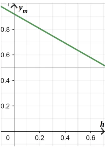
Figure 1: The proportion of the problem a manager solved y_m versus the communication costs h.

y_m = −0.571 h + 0.92 for h ∈ (0, 0.56]

y_w = 0.0357 h + 0.2 for h ∈ (0, 0.56]

Figure 1 shows that improvements in communication technology, h, lead to an increase in the proportion of a problem which a manager can solve, y_m = G(Z). As depicted, the improvements cause a manager to spend more time on solving a higher proportion of the problem, and thus her working time increases and leisure time decreases as shown in Figure 2.

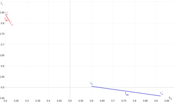
Figure 2: The leisure of agent i versus the proportion of the problem.

l_m = −0.14 y_m + 0.589 for y_m ∈ [0.6, 0.92]

l_w = −1.7 y_w + 1.18 for y_w ∈ [0.2, 0.22]

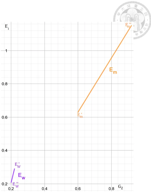
Figure 3: Earning of agent i versus the proportion of the problem.

E_m = 1.625 y_m − 0.345 for y_m ∈ [0.6, 0.92]

E_w = 4.1 y_w − 0.612 for y_w ∈ [0.2, 0.22]

In figure 2, the manager’s leisure moves from l⁰_m to l⁰⁰_m. That means her leisure time decreases because of the technology improvement. Mean- while, her earning increases because she obtains more return on problem- solving after the improvement. The upward direction of her earning is shown in Figure 3. The point moves from E_m⁰ to E_m⁰⁰ . The notable trend is the fraction of the problem a worker solved, y_w = G(Z), see Figure 3.

Observe (from point E_w⁰ to point E_w⁰⁰) in Figure 3, a worker tends to solve smaller fraction of the problem after the technology improvement.

That’s because the cost of asking a manager for directions is relatively lower than solving the problem by himself. This reduction implies a worker makes a less effort to work, and thus his leisure time increases as shown in Figure 2 (from point l_w⁰ to l_w⁰⁰). All results are shown in Ta- ble 1 and the functional forms used in this simula-tion is presented as above. Therefore, these figures illustrate that the communication tech- nology improvement leads to increases in the manager’s earning and the worker’s leisure and decreases in the manager’s leisure and the worker’s earning. That is, the improvement in communication technology leads to wage inequality and leisure inequality between high skill agents and low skill agents.

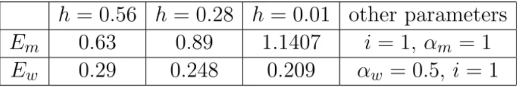
Table 1.1 Agents’ earnings before and after technology improvement h = 0.56 h = 0.28 h = 0.01 other parameters

E_m 0.63 0.89 1.1407 i = 1, α_m = 1 E_w 0.29 0.248 0.209 α_w = 0.5, i = 1

Table 1.2 Agents’ leisure before and after technology improvement h = 0.56 h = 0.28 h = 0.01 other parameters

l_m 0.505 0.482 0.461 i = 1, α_m = 1 l_w 0.806 0.823 0.839 α_w = 0.5, i = 1

To be clear, let us turn to the mathematics part. In the previous sec- tion, some functions are used to determine the equilibrium conditions.

By using the functional forms as page 16, we do comparative status to understand how the technology change affects the equilibrium quantities.

From equation (14) in Section II, the manager’s wage per unit of work- ing time is given by

(25) : w_m = 2(1 − y_w) h + 2(y_m− y_w).

If the communication technology improves, h ↓, her wage increases.

That is, the partial derivative of equation (18) with respect to h increases as

(26) : ∂w_m

∂h = − 2(1 − y_w)

(h + 2(y_m − y_w))² < 0.

Proposition 1 The improvement in communication technology leads to an increase in the manager’s wage.

As shown in Figure 1, due to improvements in communication tech- nology, the equilibrium quantities of y_m increases and y_w decreases. The following propositions is attributed to this effect:

Proposition 2 The improvement in communication technology leads to the opposite effect on production knowledge between high- and low-skilled agents: an increase in high-skilled agents’ production knowledge and an decrease in low-skilled agents’ production knowledge.

From equation (18), we have

(27) : w_m = −dc_m

dl_m = −c⁰⁰_m − c⁰_m

l⁰⁰_m − l⁰_m = c⁰⁰_m

1 − l_m⁰⁰ − c⁰_m

1 − l⁰_m > 0.

From proposition 1, we know that the wage of the manager increases.

The increase implies the marginal rate of substitution between her con- sumption and leisure rises. That is, due to the technology improvement, the manager’s consumption increases from c⁰_m to c⁰⁰_m and her leisure time declines from l_m⁰ to l_m⁰⁰ . Hence, we can obtain the following proposition:

Proposition 3 The improvement in communication technology leads to a decline in leisure for the manager.

From equation (7) in Section II, the worker’s wage per unit of working time is given by

(28) : w_w = 2 − 2y_w(1 + (i − 0.5))

4y_w .

The partial derivative of equation (29) with respect to i can be obtained by

(29) : ∂w_w

∂i = −1/2 < 0.

This derivative means a decrease in w_w is caused by an increase in the cost of acquiring production knowledge, i. Thus, for a worker, when the cost of asking a manager for help is relatively lower than learning and solving by himself, he tends to solve lower proportion of the problem, which decreases his available income on consumption. The prediction is the same as the trend in figure 3. The prediction of equation (30) leads to the following proposition:

Proposition 4 The wage of a worker decreases due to an increase in the cost of acquiring production knowledge.

According to equation (5), we have

(30) : l_w = 1 − (y_w α_w)².

As the manager’s part we discussed, if there is a reduction in the com- munication cost h, a worker tends to solve smaller fraction of the problem, y_w ↓. This decline leads to an increase in his leisure. The prediction is also the same as we showed in the previous figure. The prediction is stated with the following proposition as well:

Proposition 5 The improvement in communication technology leads to an increase in leisure for a worker.

In conclusion, our simulation is consistent with empirical findings. Leisure inequality and wage inequality between high- and low-skilled agents are caused by the improvement in communication technology.

5 Conclusion

Over decades, wage inequality and leisure inequality have dramatically increased across agents with different levels of skills. In this paper, we have explored how technology improvements affect both inequalities. [1]

states that wage inequality between high- and low-skilled agents is caused by the improvement in communication technology. Following their the- ory, our paper considers labor-leisure choices among agents. We under- stood how technology change influences leisure inequality among agents.

Our results show that improvements in communication technology lead to leisure inequality between high- and low-skilled agents besides wage inequality. Because of reductions in communication costs of solving prob- lems, the two types of agents have different decisions on their working time and leisure. That is, the low-skilled agents choose leisure more than work on their job. Oppositely, under the technology change, the high- skilled agents work more than before. Our findings are consistent with the empirical data presented in [5,6]. Of course, our work has limitations:

our theory does not include leisure goods. The goods used in leisure have been discussed in recent papers such as [7, 9]. Futhermore, our paper does not consider bargaining power between buyer and seller, and match- ing problem among the high-skilled and the low-skilled agent. It would be interesting to consider these extensions.

References

[1] Luis Garicano and Esteban Rossi-Hansberg, 2006. ”The Knowledge Economy at the Turn of the Twentieth Century: The Emergence of Hierarchies,” Journal of the European Economic Association, MIT Press, vol. 4(2-3), pages 396-403, 04-05.

[2] Luis Garicano and Esteban Rossi-Hansberg, 2012. ”Organizing growth,” Journal of Economic Theory, Elsevier, vol. 147(2), pages 623-656.

[3] U.S. Department of Labor, Bureau of Labor Statistics. 2007. Chart-

ing the U.S. Labor Market in 2006. Washington, DC: U.S. Depart- ment of Labor.

[4] Giovanni L. Violante (2008). Skill-biased technical change. Mimeo [5] Mark Aguiar and Erik Hurst, 2007. ”Measuring Trends in Leisure:

The Allocation of Time Over Five Decades,” The Quarterly Journal of Economics, Oxford University Press, vol. 122(3), pages 969-1006.

[6] Mark Aguiar and Erik Hurst, 2008. ”The Increase in Leisure Inequal- ity,” NBER Working Papers 13837, National Bureau of Economic Research, Inc.

[7] Mark Aguiar and Erik Hurst, 2009. ”A Summary of Trends in Amer- ican Time Allocation: 1965–2005,” Social Indicators Research: An International and Interdisciplinary Journal for Quality-of-Life Mea- surement, Springer, vol. 93(1), pages 57-64, August.

[8] U.S. Department of Labor, Bureau of Labor Statistics. 2010. High- lights of Women’s Earnings in 2010. Washington, DC: U.S. Depart- ment of Labor.

[9] Timo Boppart and Liwa Rachel Ngai, 2017. ”Rising inequality and trends in leisure,” CEPR Discussion Papers 12325, C.E.P.R. Discus- sion Papers.