以保結構算則求解非線性薛丁格方程

國立臺灣大學理學院應用數學科學研究所

碩士論文

Institute of Applied Mathematical Sciences College of Science

National Taiwan University Master Thesis

以保結構算則求解非線性薛丁格方程

Application of a Structure-preserving Scheme to Solve Nonlinear Schrödinger Equation

紀露結 Loke-Keat Kee

指導教授：許文翰 博士

Advisor: Tony Wen-Hann Sheu, Ph.D.

Abstract

Rogue wave has been captivating to researchers. People have not fully understood rogue wave yet. The first strong scientific evidence was presented in 1995, just nearly a quarter-century ago. Since then, people gradually noticed that this phenomenon could occur in other media as well. The first optical rogue wave was reported in 2007.

In the first part of this thesis, we try to understand this special phenomenon. The definition of rogue wave is introduced and then the physical mechanisms of rogue wave are given according to linear mechanism and nonlinear mechanism. From the nonlinear

mechanism, nonlinear Schrödinger equation (NLS) can be obtained analytically. We would like to know more about rogue wave by investigating NLS equation. Similarly, the coupled NLS equations are obtained by considering the linear and nonlinear response in the

birefringent optical fibers. The coupled NLS equations can describe the pulse propagation in those fibers.

In the second part of this thesis, we review a numerical method that can solve NLS equation for which the equation is separated into linear and nonlinear part. The latter can be solved iteratively. The method has been modified in order to solve coupled NLS equations.

In the third part of this thesis, we first consider examples that admit exact solutions in

order to know the proposed algorithms work well in both NLS and coupled NLS cases. We

then move to solve semi-classical NLS equation by using this method. Last but not least, we

simulate rogue wave and two quantized vortex lattices in a rotating trapped Bose-Einstein

condensate (BEC). We hope to know more about these phenomena through simulations.

中文摘要

摘要瘋狗浪較普通海浪高出一倍以上。在沒有電子儀器的航海時代，瘋狗浪被斥為無

稽之談——能在此滔天巨浪中倖存之人不多，加之當時學界普遍認為海浪高不過 30 英

呎（9.1m）。1995 年元旦，在大西洋北海的鑽油台上，靈敏的電子儀器記錄到了以時

速 72.4 公里撲打平台的巨浪，其浪高 25.9m，足足較當時週遭的海平面有效波高高出

13.9m。瘋狗浪這一現象也會在海波之外的介質中出現。2007 年，科學家們發現了光 學中的瘋狗浪，此一成果發表在《自然》期刊上。

摘要在本論文的第一部份，我們嘗試從線性與非線性兩種機制來瞭解瘋狗浪這一現

象。從非線性機制中，可推導出非線性薛丁格方程式。同樣地，在光纖的雙折射現象 中，我們可以推導出耦合的非線性薛丁格方程式。

摘要在論文的第二部份，我們將討論能解此非線性薛丁格方程式的數值方法。其中，

非線性薛丁格方程式被分為線性與非線性兩部份，在數值求解時交替解之。另外，此 數值方法也可解耦合的非線性薛丁格方程式。

摘要論文的第三部份則給出了數值結果。首先是帶有實解的例子，我們能由此得知程

式是否無誤。接著我們解了半古典（semi-classical）的非線性薛丁格方程式。最後我 們嘗試模擬瘋狗浪以及旋轉玻色－爱因斯坦凝聚中的兩個量子化渦格。

關鍵字：瘋狗浪；非線性薛丁格方程式；耦合非線性薛丁格方程式。

Contents

Abstract i

1 Introduction 1

1.1 Rogue wave . . . 1

1.2 Birefringent optical fibers . . . 2

2 Physical mechanisms of rogue wave 4 2.1 Linear mechanism . . . 4

2.1.1 Spatial focusing . . . 4

2.1.2 Dispersive focusing . . . 5

2.2 Nonlinear mechanism . . . 5

2.2.1 Weakly nonlinear waves . . . 5

2.2.2 Modulation instability . . . 7

2.3 Conservation laws . . . 10

3 Derivation of coupled NLS equation from birefringent optical fibers 14 3.1 Linear Response . . . 14

3.2 Nonlinear Response . . . 18

3.3 Normalization . . . 19

3.4 Exact Solution . . . 20

4 Numerical method 23 4.1 Solving one-dimensional NLS equation . . . 23

4.1.1 Linear part . . . 23

4.1.2 Nonlinear part . . . 30

4.2 Solving two coupled NLS equations . . . 31

5 Verification studies 33 5.1 Classical NLS equation . . . 33

5.2 Semi-classical NLS equation . . . 37

5.3 Coupled NLS equations . . . 45

5.4 Rogue wave simulation . . . 50

5.5 Nonlinear optical wave simulation . . . 52

6 Concluding remarks 55

Bibliography 56

List of Tables

1 Errors between the exact solution and the numerical solution in example 1. . . 33 2 Errors between the exact solution and the numerical solution in example 2. . . 34 3 Errors between the exact solution and the numerical solution in example 3 . . . 35 4 Errors between the exact solution and the numerical solution of Ψ1and Ψ2in example

7. . . 46

List of Figures

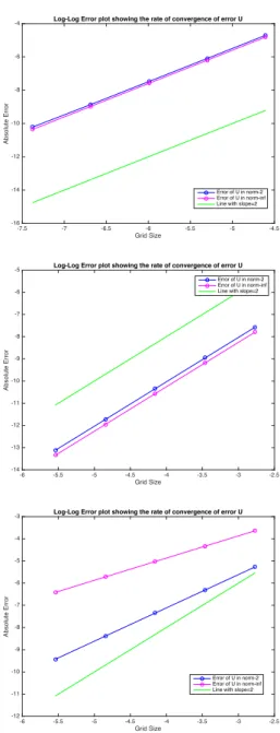
1 k∆x versus k∆x for the DRP fourth-order central finite difference scheme of u˜ x . . . 27 2 The log-log error plot of example 1, 2 and 3. The rate of convergence in space in

the first two one-dimensional examples is around 2. However, when it comes to the two-dimensional case the rate of convergence in space is slightly decreased to 1.5. . . 36 3 On the left is the mass density |u|², on the right is the momentum density J at time

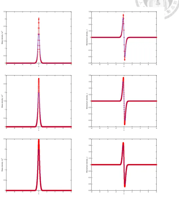
t = 0.5. ε decreases from top to bottom: ε = ₂₀¹,₄₀¹,₈₀¹ while ∆x decreases at the same magnitude as well: ∆x = ₃₂¹,₆₄¹,₁₂₈¹ . ∆t = 0.2(∆x)²holds for these cases. Red line with dots represents the numerical result for each ε while blue line represents the weak limit for ε → 0. . . 38 4 (Continued) On the left is the mass density |u|², on the right is the momentum

density J at time t = 0.5. ε decreases from top to bottom: ε = ₁₆₀¹ ,₃₂₀¹ while ∆x decreases at the same magnitude as well: ∆x = ₂₅₆¹ ,₅₁₂¹ . ∆t = 0.2(∆x)² holds for these cases. Red line with dots represents the numerical result for each ε while blue line represents the weak limit for ε → 0. . . 39 5 A closer look at the mass density |u|². Top: from time t = 0 to t = 0.5, |u|² is

increasing as time advances. Bottom: from time t = 0.5 to t = 0.9, the growth of

|u|²is even dramatic. . . 40 6 The plot of the compressive initial data _dx^dS0(x) = − tanh(5(x − 0.5)) for x ∈ [0, 1] . 41

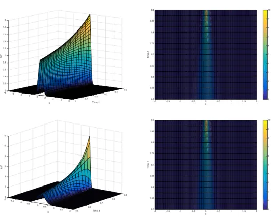
7 On the left is the mass density |u|², on the right is the momentum density J at time t = 0.54. ε decreases from top to bottom: ε = 0.0256, 0.0064, 0.0016 while ∆x decreases at the same magnitude as well: ∆x = ₃₂¹,₁₂₈¹ ,₅₁₂¹ . ∆t = 0.2(∆x)² holds for these cases. . . 42 8 The Riemann invariant r+ at different times at t = 0.0, 0.2, 0.4, 0.6, 0.8, 1.0. The

peak at x = 0 is getting higher as time advances. . . 44 9 Top: The initial mass density ρ(x, 0) (left) and momentum density J(x, 0) (right).

Bottom: At time t = 1.0, the mass density and momentum density both have become steeper at x = 0. Red line with dots represents the numerical result while blue line represents the initial conditions. . . 44 10 The log-log error plots of Ψ1and Ψ2in example 7. The rate of convergence in space

for both solutions is around 2. . . 46 11 The simulated space-time plot when the collision of two solitons happens. . . 47 12 We can see that at time t = 0.4, two solitons which have the initial amplitudes

α1 = 1, α2 = 0.5 are moving towards each other. At time t = 0.8, they start to interact. . . 48 13 At time t = 1.0 the two solitons have collided and superpositions happen. At a time

around t = 1.6 the two solitons have separated from each other. . . 49 14 The simulated |u| is plotted in space-time diagrams. . . 50 15 From time t = 0 to time t = 2.27, 3.32, 4.85, 7.40, 8.40, the distributions of |u| are

plotted. . . 51 16 From time t = 0 to time t = 0.16, the contour surfaces of |Ψ1(x, y, t)|²are plotted. . 53 17 From time t = 0.2 to time t = 0.5, the contour surfaces of |Ψ1(x, y, t)|²are plotted. . 54

1 Introduction

1.1 Rogue wave

Rogue wave is dangerous due to its unexpected large surface waves. It appears suddenly and disappear without leaving a trace [1]. Not many mariners could survive and even they did, the eyewitness accounts were seldom taken into consideration. It was widely believed that no waves could exceed 9 meters in eighteen and nineteen century.

Rogue wave was first introduced to scientific community by Laurence Draper in 1964 [2]. How- ever, not until twenty years later the first scientific evidence was recorded at the Gorm platform in the central North Sea. The wave height was 11 meters in a relatively low sea state. On the first day of 1995, a strong scientific evidence was received at the Draupner platform in the North Sea and immediately it caught everyone’s attention. A wave with the astonishingly height of 25.9 meters was recorded by all of the sensors fitted to the platform. It is now known as “Draupner wave” or

“New Year’s Wave” [3].

Nowadays the existence of rogue wave can be confirmed by video and photographs, and even satellite imagery and radar of the ocean surface. In 2004, ten rogue waves were found in a limited area of the South Atlantic within three weeks using radar images from European Space Agency(ESA) satellites. Their heights were all above 25 meters. This ESA MaxWave project confirmed the widespread existence of rogue waves.

Though rogue wave is now generally noticeable, there is no unique definition of such wave.

A rogue wave is defined in pragmatic approach whenever the wave height H exceeds a certain threshold based on the background sea state defined by the significant wave height Hs,

H Hs > 2

where wave height H is the total vertical distance from the wave trough to the wave crest. On the other hand, significant wave height is traditionally defined as the average of the one-third largest waves and denoted H_1/3. Today it is taken as four times the standard deviation of the surface

elevation and denoted as Hs. There is also another common criterion using crest height ηc

ηc

Hs > 1.25

where crest height is the vertical distance from the mean water level to the crest.

Despite the height generated, rogue wave is distinct from tsunami. Tsunami is caused by the displacement of a large volume of water, often resulting from a sudden movement of the ocean floor.

Tsunami has longer wavelength and propagate at high speed over a wide area. It is often less than one meter high and nearly unnoticeable in deep water. When tsunami enters shallow water, it slows down and the height grows enormously due to shoaling effect. Thus, tsunami becomes dangerous as it approaches the shoreline while rogue wave is normally dangerous to ships in the open ocean.

Rogue wave can be found in media other than water. They have been sought experimentally and studied in large wave tanks [4], optical systems [5], and superfluid ⁴He [6]. A recent review paper even discusses different media in which rogue wave can occur [7]. Although rogue wave seems to be quite common in nature, we have little knowledge about the origins of rogue wave from the ocean. During the last 30 years various physical models of the rogue wave phenomenon have been intensively developed. The main goal is to understand the physics of the rogue wave and to provide the design of rogue wave needed for engineering purposes. In next section, we shall discuss several possible mechanisms of rogue wave.

1.2 Birefringent optical fibers

An optical fiber is a flexible, transparent fiber made by drawing glass or plastic to a diameter slightly thicker than that of a human hair. In fiber-optic communication, a single-mode optical fiber is an optical fiber designed to carry light in a single ray. It is often called transverse mode since its electromagnetic vibrations occur perpendicular which is transverse to the length of the fiber. The 2009 Nobel Prize in Physics was awarded to Charles K. Kao for his theoretical work on the single-mode optical fiber.

However, single-mode fibers in practice do not contain single mode. The fibers are actually bimodal due to the presence of birefringence. Birefringence is the property of optically non-isotropic

transparent materials that the refractive index depends on the polarization direction which is the direction of the electric field. Birefringence can result from an elliptical shape of the fiber core, from other asymmetries of the fiber design, or from mechanical stress, for example, bending or random perturbations.

In an ideal circular-core fiber, these two modes will propagate with the same phase velocity but practical fibers are not perfectly circularly symmetric. As a result, the two modes propagate with slightly different phase and group velocities. Hence, birefringence can cause pulse splitting which is bad in communication applications. While on the other hand, environmental factors such as bend, twist, and non-isotropic stress will couple energy from one mode to the other mode of the fiber, creating problems in practical applications.

In section 3, we shall derive equations describing pulse propagation in birefringent optical fibers which is the coupled nonlinear Schr¨odinger equation.

2 Physical mechanisms of rogue wave

Several suggestions have been raised to explain the mechanisms leading to rogue wave such as the combined effects of wind and currents, and the focusing effects associated with the topology of the ocean floor and nearby shorelines. However, rogue wave will also appear in deep ocean. It is hinted that rogue wave may evolve though a nonlinear interaction process as well.

2.1 Linear mechanism

Rogue wave can be formed owing to a simple consequence of linear superposition of waves [8].

These waves have small-amplitude, different frequencies and different directions of propagation.

Linear theory, however, is based on the assumption that the wave components are harmonic and independent from each other. When the waves are too steep, the linear wave theory is no longer valid. On the other hand, dispersive focusing is the linear mechanism that was proposed in 1980s.

It could be used to produce rogue waves in water tank. Such mechanism has not yet been identified in ocean.

2.1.1 Spatial focusing

Spatial focusing is caused by wave refraction and diffraction. Different geometrical shapes of seabed and costal lines can result in energy focusing of waves. Probability of the occurrence of rogue wave might then increase. A notorious example is the big waves observed in the Agulhas current. In African southeast coast, the Agulhas current encounters the westerlies. The wind blowing from the west in this case can be considered as the initial condition for the wave system in Agulhas current.

Strong winds from a storm may cause waves to be focused and caustic and, hence, turn into rogue wave at random location and time. This represents the rare and short-lived character of rogue wave.

2.1.2 Dispersive focusing

Gravity waves are dispersive. The phase and group velocities of gravity waves are inversely pro- portional to the frequency. Longuet-Higgins (1974) applied this mechanism to create short groups of large waves at a given position in a wave tank [9]. The idea to produce such waves is to use a linearly decreasing frequency known as chirp. When the chirp is properly selected, this group of waves starts to disperse and decreases to a few wavelengths for which the waves turn to have a larger amplitude. This kind of dispersive focusing phenomenon has been suggested by Kharif and Pelinovsky as a possible mechanism leading to rogue waves[10].

2.2 Nonlinear mechanism

Linear theory works only when the wave components are harmonic and independent. If the waves are too steep, the nonlinear contribution becomes significant and hence the linear wave theory fails.

Weakly nonlinear theory has been widely used to explain the existence of rogue waves [11]. Several mathematical models have been developed for the study of deep-water waves. Among them, the nonlinear Schr¨odinger equation, first derived by Zakharov in 1968 [12], is preferable and will be used in our discussion.

2.2.1 Weakly nonlinear waves

Consider a wave with the amplitude A(x, t) and phase Φ(x, t) and suppose they change slowly with time. The wave function at the position x and time t can be written as

u(x, t) = A(x, t)e−i(Φ(x,t)−ωt)

and a slowly varying envelope approximation can be made and the surface elevation up to first order of nonlinearity can be written as

η(x, t) = 1 2

!A(x, t)e^{−i(k0x−ω0t)}+ A^∗(x, t)e^{i(k0x−ω0t)}"

where k0, ω0 are the wave number and frequency of the carrier wave with ∗ denotes the complex conjugate.

The complex envelope A(x, t) obeys the nonlinear model of deep-water wave trains. It can be written in the lowest order in wave steepness and spectral width:

i!∂A

∂t + vg

∂A

∂x

"

− ω0

8k²₀

∂²A

∂x² −1

2ω0k²₀|A|²A = 0 (1) where vg = ^∂ω_∂k is the group velocity. The second term of this equation takes into account the dispersive behaviour of the surface elevation while the last term is the nonlinear term. This is the space nonlinear Schr¨odinger equation (space NLS). It describes the space/time dynamics of the complex envelope function A(x, t) of a deep-wave train which propagates in the x-direction as a function of time.

Since x = vgt, we can rewrite the space nonlinear Schr¨odinger equation into time nonlinear Schr¨odinger equation (time NLS):

∂A

∂t = vg

∂A

∂x

∴∂²A

∂x² = 1 v_g²

∂²A

∂t² The time NLS equation is hence

i!∂A

∂t + vg∂A

∂x

"

− ω₀ 8k²₀· 1

v_g²

∂²A

∂t² −1

2ω0k₀²|A|²A = 0 i!1

vg

∂A

∂t +∂A

∂x

"

− ω0

8k²₀v_g³

∂²A

∂t² −ω0k²₀

2vg |A|²A = 0 i!∂A

∂x + 1 vg

∂A

∂t

"

− k0

ω²₀

∂²A

∂t² − k0³|A|²A = 0 (2) where we have used the knowledge that in deep water wave, the ratio of group velocity vg to the phase velocity vp=^ω_k is ¹₂.

On the other hand, we can also transform the space NLS equation into dimensionless equation

by setting

X = x − vgt T = t

ξ = 1

√2ω0k0A0X

τ = −k0³A²₀T u = A

A0

Thus, substitute the setting above into (1), we obtain the dimensionless space NLS

i∂u

∂τ +1 2

∂²u

∂ξ² + |u|²u = 0

For convenience, we shall write the dimensionless space NLS using x, t as the space and time variable instead of ξ and τ

i∂u

∂t +1 2

∂²u

∂x²+ |u|²u = 0 (3)

2.2.2 Modulation instability

The phenomenon of modulation instability has been observed in different physical systems including plasmas [13], laser light [14], and Bose-Einstein condensation [15]. This phenomena was discovered theoretically and experimentally in various studies conducted in the 1960s [16].

In the context of water waves, the study was pioneered by the works of Whitham [17], Lighthill [18], Benjamin and Feir [19]. This phenomenon is named after Benjamin and Feir because they were the first in discovering the sideband nature of the instability. They showed that this instability occurs if kh > 1.363 where k is the wave number and h is the water depth. They also demonstrated the instability in a laboratory water tank for the first time.

We shall now investigate the modulational instability in NLS equation with the form

i∂u

∂t + β∂²u

∂x²+ γ|u|²u = 0

where the parameter β describes the group velocity dispersion and γ represents the magnitude of Kerr nonlinearity. Suppose we have a periodic waveform of constant power P , that is

u(x, t) =√ P e^{iγP t}

To obtain the perturbation equation, we start by perturbing the solution

˜

u(x, t) =!√

P + ϵ(x, t)"

e^{iγP t}

where ϵ(x, t) is the perturbation term. Substitute ˜u(x, t) into NLS equation gives us

i∂ϵ

∂t+ β∂²ϵ

∂x² + γ(ϵ + ϵ^∗)P + γ√ P!

ϵ²+ 2|ϵ|²"

+ γ|ϵ|²ϵ = 0

Since the perturbation should be small, we assume |ϵ| ≪ √

P so that the last two terms can be dropped out:

i∂ϵ

∂t+ β∂²ϵ

∂x²+ γ(ϵ + ϵ^∗)P = 0

If the solutions of this perturbation equation grow exponentially, then instability will occur. Con- sider the solution of this perturbation equation has the form

ϵ(x, t) = ce^{−i(kmx−ωmt)}+ c^∗e^{i(kmx−ωmt)}

where c is the constant with ∗ denotes the complex conjugate and km, ωmare the wavenumber and angular frequency of the perturbation respectively. It is easy to see that both kmand ωmmust be real-valued. Otherwise, there will be an exponential growth in ϵ(x, t).

Substitute this ϵ(x, t) into the perturbation equation above and we get

ω²_m= k²_m(β²k_m² − 2γβP )

Since ωmis real-valued, we must have

k_m²(β²k_m² − 2γβP ) ≥ 0

Otherwise, when ωmis complex, which is

k_m²(β²k_m² − 2γβP ) < 0

we would have instability. This means that the instability happens when

k²_m< 2γP β For the NLS equation

i∂u

∂t +∂²u

∂x²+ 2|u|²u = 0 (focusing) i∂u

∂t +∂²u

∂x²− 2|u|²u = 0 (defocusing)

we see that the modulational instability happens in the focusing case. We will try to simulate rogue wave later using

i∂u

∂t +∂²u

∂x²+ 2|u|²u = 0 with u(x, 0) = sech^x₆ where

k²_m< 2γP

β = 4sech²x 6 < 4 On the other hand, we shall have another look at the instability:

i∂u

∂t + β∂²u

∂x²+ γ|u|²u = 0 and the solution in the form

u(x, t) =√ P e^{iγP t} we see that the instability happens when

k²_m< 2γP β

That is, if γP is large (fast oscillation) or β is small, the instability will be likely to happen. Hence, we could study the initial value problem

iεut+ε²

2uxx+ |u|²u = 0

with u(x, 0; ε) = A(x)e^εiS(x) where ε > 0 is a small parameter, A(x) and S(x) are real-valued smooth functions.

If we let

m = |u|² n = ε 2i

!u_x u −u^∗_x

u^∗

"

the initial value problem can be written as

mt+ (mn)x= 0 n_t+ nm_x− mx= −ε²

4

!1 2

u²_x u²−uxx

u

"

x

with initial data not depending on ε

m(x, 0) = A²(x), n(x, 0) = S^′(x)

The modulational instability comes from ε → 0.

2.3 Conservation laws

For now we shall consider the following dimensionless nonlinear Schr¨odinger equation to model rogue wave in deep water

iεut+ε² 2uxx−!

f (|u|²) + V (x)"

u = 0. (4)

where f is a real-valued smooth function and V (x) is a given real-valued electrostatic potential and u(x, t) is the wave function. The small free parameter ϵ with 0 < ϵ ≪ 1 denotes the modulation scale. The wave function can be used to compute primary physical quantities such as the mass density

ρ(x, t) = |u(x, t)|² the momentum density

J(x, t) = εIm(u^∗(x, t)∇u(x, t)) = ε

2i(u^∗∇u − u∇u^∗) and energy density

E(x, t) =ε²

2|∇u(x, t)|²+ V (x)|u(x, t)|²

where the “*” denotes complex conjugation. The solution of the self-focussing nonlinear Schr¨odinger equation (4) will be sought later in the semiclassical limit. Our interest stems from the existence of modulationally unstable solution behavior.

In this section we shall obtain the conservation laws of mass density and momentum density in one dimension. This will help us to analyze and understand the mechanism of the solution. We start by considering simpler case where the potential V (x) is zero

iεut+ε²

2uxx− U^′(|u|²)u = 0. (5)

We have also assumed f (|u|²) = U^′(|u|²) to be a twice differentiable nonlinear real-valued function.

The local conservation laws are then

∂ρ

∂t +∂J

∂x = 0 (6)

∂J

∂t + ∂

∂x

!J² ρ

"

+∂P (ρ)

∂x = ε² 4

∂

∂x

! ρ ∂²

∂x²log ρ"

(7)

where P (ρ) = ρU^′(ρ) − U(ρ).

To obtain the first conservation law (6), we first eliminate U^′(|u|²)u by multiplying the complex conjugate of u to (5). On the other hand, we take the complex conjugate of (5) and multiply −u to it. These both give

iεu^∗u_t+ε²

2u^∗u_xx− U^′(|u|²)u^∗u = 0 iεuu^∗_t−ε²

2uu^∗_xx+ U^′(|u|²)u^∗u = 0 Adding them together we will have

iε!

u^∗ut+ uu^∗_t"

+ε² 2

!

u^∗uxx− uu^∗xx

"

= 0

⇒!

u^∗ut+ uu^∗_t"

−iε 2

!u^∗uxx+ u^∗_xux− u^∗xux− uu^∗xx

"

= 0

⇒ ∂

∂t#uu^∗$ −iε 2

∂

∂x

!

u^∗ux− uu^∗x

"

= 0

⇒ ∂

∂tρ(x, t) + ∂

∂xJ(x, t) = 0

where J(x, t) = −^iε₂!

u^∗ux− uu^∗x

"

in one dimension.

To obtain the second conservation law (7), we first take the derivative of J(x, t) with respect to time.

∂

∂tJ(x, t) = −iε 2

!u^∗_tux+ u^∗uxt− utu^∗_x− uu^∗xt

"

Since iεu_t+^ε₂²u_xx− U^′(ρ)u = 0, we have

iεut= −ε²

2uxx+ U^′(ρ)u

−iεu^∗t = −ε²

2u^∗_xx+ U^′(ρ)u^∗ iεutx= −ε²

2uxxx+ U^′′(ρ)ρxu + U^′(ρ)ux

iεu^∗_tx= ε²

2u^∗_xxx− U^′′(ρ)ρxu^∗− U^′(ρ)u^∗_x Plugging them into the time derivative of J(x, t) we see that

∂

∂tJ(x, t) + ∂

∂xP (ρ) = −ε²

4Q(u, ux, uxx) (8)

where P (ρ) = ρU^′(ρ) − U(ρ) and Q(u, ux, uxx) = 2ux+ u^∗_x− uu^∗xx− u^∗uxx. On the other hand,

ρ = uu^∗ ρx= uxu^∗+ uu^∗_x (ρ_x)²= (u_xu^∗+ uu^∗_x)²

= (u_xu^∗− uu^∗x)²+ 4uu^∗u_xu^∗_x

∴(uxu^∗− uu^∗x)²= (ρx)²− 4ρuxu^∗_x

⇒!

− 2 iεJ"2

= (ρx)²− 4ρuxu^∗_x

∴ J² ρ =ε²

4

!−(ρx)²

ρ + 4u_xu^∗_x"

=ε² 4

%

ρ ·ρρxx− (ρx)²− ρρxx

ρ² + 4uxu^∗_x

&

=ε² 4

% ρ ∂

∂x

!ρx

ρ

"

− ρxx+ 4uxu^∗_x

&

=ε² 4

% ρ ∂²

∂x²log ρ − uxxu^∗− uu^∗xx+ 2uxu^∗_x

&

∴ ∂

∂x

!J² ρ

"

=ε² 4

∂

∂x

% ρ ∂²

∂x²log ρ

&

+ε²

4Q(u, ux, uxx) Adding (8) to the equation above, we obtain

∂J

∂t + ∂

∂x

!J² ρ

"

+∂P (ρ)

∂x = ε² 4

∂

∂x

! ρ ∂²

∂x²log ρ"

These two conservation equations have the form of a perturbation of the compressible Euler equa- tions of fluid dynamics with the pressure P (ρ). If the Euler part of these equations is to be hyper- bolic, then the pressure P (ρ) must be a strictly increasing function of ρ, that is P^′(ρ) = ρU^′′(ρ) > 0.

This implies U must be a strictly convex function of ρ and this corresponds to a defocusing NLS case.

On the other hand, for the focusing NLS case, we must have P^′(ρ) = ρU^′′(ρ) < 0. This means that when the mass density ρ increases, the pressure P (ρ) decreases. Thus there will be a phenomenon leading to the development of mass concentrations.

Also on the right hand side, we have the O (ε²) dispersive term. If the mass density ρ(x, t) and momentum density J(x, t) have a singularity, then the small dispersive term can no longer be negligible since it will develop a small wavelength oscillations.

3 Derivation of coupled NLS equation from birefringent op- tical fibers

We shall follow the derivation in [20] and start from Maxwell’s wave equation for plane waves

∂²E

∂z² − 1 c²

∂²D

∂t² = 0 (9)

where E is the electric field, D is the dielectric response, c is the speed of light, z and t are the propagation distance and time. The relationship of dielectric response and electric field is given by

D= E + 4πP

where P is the polarizability. Note that E and D are observed fields which means E, D, P are real.

The next task is to decide the relationship of P and E. We shall consider the linear response and nonlinear response separately and combine them into Maxwell’s wave equation in order to derive the equations describing pulse propagation in birefringent optical fibers.

3.1 Linear Response

For the linear response, we shall assume that the medium is non-isotropic. This means that the medium is birefringent along the z-direction. Thus, PLand E are related through a tensor χ

PL(z, t) = ' t

−∞χ(t − ˜t) · E(z, ˜t)d˜t (10)

We now consider the Fourier transforms of E, PLand χ. In general, f (z, ω) =ˆ

' _∞

−∞

f (z, t)e^iωtdt

and

f (z, t) = 1 2π

' _∞

−∞

f (z, ω)eˆ ^−iωtdω. (11)

We shall define

fˆ⁺(z, ω) =

⎧

⎪⎪

⎨

⎪⎪

⎩

f (z, ω),ˆ ω > 0

0, ω < 0

(12)

and ˆf⁻(z, ω) = ˆf (z, ω) − ˆf⁺(z, ω). The corresponding quantities f⁺(z, t) and f⁻(z, t) are then defined by (11). Following this, we have defined the terms E^±(z, ω), ˆE^±(z, ω) and so on. Hence we can rewrite the linear response

Pˆ⁺(z, ω) = ˆχ⁺(ω) · ˆE⁺(z, ω) (13)

Here we shall assume that the nonzero contribution to E and D comes from a small region in ω space surrounding some carrier frequency ω0 and another small region surrounding its opposite

−ω0. Since E(z, t) is real, we always have ˆE(z, −ω) = ˆE^∗(z, ω). This implies we can simply consider the positive frequency components in the small region around ω = ω₀ and restore the negative frequency components at the end of calculation.

Next, we shall write

Eˆ⁺= ˆE⁺₁e₁+ ˆE₂⁺e₂ (14) Pˆ⁺= ˆP₁⁺e₁+ ˆP₂⁺e₂ (15)

where e₁, e₂ are the two orthonormal eigenvectors of ˆχ⁺ at any arbitrary frequency ω with the corresponding eigenvalues χ1and χ2. This gives us

Pˆ₁⁺= ˆP⁺e₁=#Eˆ⁺· ˆχ⁺$e₁= χ1Eˆ⁺e₁= χ1Eˆ₁⁺ (16) Pˆ₂⁺= ˆP⁺e₂=#Eˆ⁺· ˆχ⁺$e₂= χ2Eˆ⁺e₂= χ2Eˆ₂⁺ (17)

where e₁· e1∗= e₂· e2∗= 1 and e₁· e2∗= 0. We may further assume that in the positive small region in ω space, e₁(ω) = e₁(ω0) and e₂(ω) = e₂(ω0) so as to ignore the coupling of linear mode.

We then have

P₁⁺(z, t) = ' t

−∞

χ1(t − ˜t)E1⁺(z, ˜t)d˜t (18)

P₂⁺(z, t) = ' t

−∞

χ2(t − ˜t)E2⁺(z, ˜t)d˜t (19) If we let

P₁⁺(z, t) = ρ(z, t)e^ik0z−iω0t (20) E⁺₁(z, t) = U (z, t)e^ik0z−iω0t (21)

where ρ and U are the envelopes of P₁⁺ and E₁⁺ with k0 = k(ω0) given by the linear dispersion relations corresponding to the eigenmodes of ˆχ⁺

k(ω) = ω

c,1 + 4π ˆχ1(ω) = ω

c, ˆϵ1 (22)

l(ω) =ω

c,1 + 4π ˆχ2(ω) = ω

c, ˆϵ2 (23)

Substitute (20) and (21) into (18), we obtain ρ(z, t) =

' t

−∞

χ1(t − ˜t)U(z, ˜t)e^{iω0(t−˜t)}d˜t

= ' ∞

0

χ1(s)U (z, t − s)e^iω0sds

= ' ∞

−∞

χ1(s)U (z, t − s)e^iω0sds

= ' ∞

−∞

! 1 2π

' ∞

−∞

ˆ

χ1(ω)e^−iωsdω"

U (z, t − s)e^iω0sds

= 1 2π

' _∞

−∞

' _∞

−∞

ˆ

χ1(ω)U (z, t − s)e^{−i(ω−ω0)s}dωds

= 1 2π

' _∞

−∞

' _∞

−∞

ˆ

χ1(ω + ω0)U (z, t − s)e^−iωsdωds

= 1 2π

' _∞

−∞

ˆ

χ1(ω + ω0)!' _∞

−∞U (z, t − s)e^iω(t−s)ds"

e^−iωtdω

= 1 2π

' ∞

−∞

ˆ

χ1(ω + ω0)!' ∞

−∞

U (z, t^∗)e^iωt∗dt^∗"

e^−iωtdω

= 1 2π

' ∞

−∞

ˆ

χ1(ω + ω0) ˆU (z, ω)e^−iωtdω

In order to integrate the equation above, we approximate ˆχ1(ω + ω0) at ω0

ˆ

χ1(ω + ω0) ≈ ˆχ1(ω0) + ˆχ^′₁(ω0)ω +1

2χˆ^′′₁(ω0)ω² while ˆU (z, ω) is zero outside the small region of ω0, we see that

ρ(z, t) ≈ 1 2π

' _∞

−∞

! ˆ

χ1+ ˆχ^′₁ω +1

2χˆ^′′₁ω²" ˆU e^−iωtdω

= ˆχ1· 1 2π

' _∞

−∞

U eˆ ^−iωtdω + ˆχ^′₁· 1 2π

' _∞

−∞

ω ˆU e^−iωtdω +1 2χˆ^′′₁· 1

2π ' _∞

−∞

ω²U eˆ ^−iωtdω

= ˆχ1U + i ˆχ^′₁· 1 2π

' _∞

−∞−iω ˆUe^−iωtdω −1 2χˆ^′′₁· 1

2π ' _∞

−∞(−iω)²U eˆ ^−iωtdω

= ˆχ₁U + i ˆχ^′₁∂U

∂t −1 2χˆ^′′₁∂²U

∂t²

Till now, we have reduced all relationship to U , in order to obtain the equation linearly describing pulse propagation in birefringent optical fibers, we first assemble D⁺₁ by substituting ρ(z, t) into P₁⁺

D⁺₁ = E₁⁺+ 4πP₁⁺

= U (z, t)e^ik0z−iω0t+ 4πρ(z, t)e^ik0z−iω0t

=-

U + 4π! ˆ

χ1U + i ˆχ^′₁∂U

∂t −1 2χˆ^′′₁∂²U

∂t²

".

e^ik0z−iω0t

=-

(1 + 4π ˆχ1)U + i ˆχ^′₁∂U

∂t −1 2χˆ^′′₁∂²U

∂t² .

e^ik0z−iω0t

=! ˆ

ϵ₁U + iˆϵ^′₁∂U

∂t −1 2ˆϵ^′′₁∂²U

∂t²

"

e^ik0z−iω0t

where ˆϵ1= 1 + 4π ˆχ1has been previously defined in the linear dispersion relation. Hence plugging D⁺₁ and E⁺₁ into the Maxwell’s wave equation

∂²E₁⁺

∂z² − 1 c²

∂²D⁺₁

∂t² = 0 we obtain

!− k²0+ω²₀ˆϵ1

c²

"

U + 2ik₀∂U

∂z + i!2ω0ϵˆ1+ ω²₀ˆϵ^′₁ c²

"∂U

∂t +∂²U

∂z² −!ˆϵ1+ 2ω0ˆϵ^′₁+¹₂ω²₀ˆϵ^′′₁ c²

"∂²U

∂t² = 0 (24) where we have omitted the third order and fourth order time derivatives. Since k(ω) = ^ω_c,ˆϵ1(ω) we see that

k²₀= ω₀² c²ϵˆ1

k^′= 2ω0ˆϵ1+ ω₀²ˆϵ^′₁ 2k0c²

k^′′= 2ˆϵ1+ 4ω0ϵˆ^′₁+ ω₀²ˆϵ^′′₁− 2c²(k^′)² 2k0c²

This yields (24) can be simplified

i!∂U

∂z + k^′∂U

∂t

"

+ 1 2k₀

∂²U

∂z² −!ˆϵ1+ 2ω0ˆϵ^′₁+¹₂ω₀²ˆϵ^′′₁ 2k₀c²

"∂²U

∂t² = 0 (25)

Since U is slowly varying in time and space, we require ^∂U_∂z and ^∂U_∂t to be in the same order, that is

∂U

∂z + k^′∂U

∂t ≡ 0

This gives

∂²U

∂z² = (k^′)²∂²U

∂t² Thus, (25) can further be simplified as

i!∂U

∂z + k^′∂U

∂t

"

−!ϵˆ₁+ 2ω₀ϵˆ^′₁+¹₂ω²₀ˆϵ^′′₁− c²(k^′)² 2k0c²

"∂²U

∂t² = 0 i∂U

∂z + ik^′∂U

∂t −1 2k^′′∂²U

∂t² = 0 (26)

Similarly, if we let

E₂⁺(z, t) = V (z, t)e^il0z−iω0t we will have

i∂V

∂z + il^′∂V

∂t −1 2l^′′∂²V

∂t² = 0 (27)

3.2 Nonlinear Response

For the nonlinear response, we shall consider third order nonlinearity due to Kerr effect for which the polarizability is in the form

P_NL(z, t) = ' t

−∞

' t

−∞

' t

−∞

χNL(t − t1, t − t2, t − t3) ·/E(z, t₁) · E(z, t2)0E(z, t₃)dt3dt2dt1 (28)

We now make the assumption that the nonlinearity is rapid compared to ω⁻¹₀ or the period of the light. Thus, we have

¯ χNL=

' t

−∞

' t

−∞

' t

−∞

χNL(t − t1, t − t2, t − t3)dt3dt2dt1

The equation (28) can now be written

PNL(z, t) = ¯χNL/E(z, t) · E(z, t)0E(z, t) (29)

As in linear response, we shall consider the the contribution of PNL in positive small region con- centrated near ω = ω0, by taking P⁺

P⁺(z, t) = ¯χ_NL/2E⁺(z, t) · E⁻(z, t)0E⁺(z, t) + ¯χ_NL/E⁺(z, t) · E⁺(z, t)0E⁻(z, t)

The first component in P⁺is

P₁⁺(z, t) = P⁺(z, t)e₁

= ¯χNL/2E⁺(z, t) · E⁻(z, t)0E⁺(z, t)e₁+ ¯χNL/E⁺(z, t) · E⁺(z, t)0E⁻(z, t)e₁

= 2 ¯χNL

!

E⁺₁E₁⁻+ E₂⁺E₂⁻"

E⁺₁ + ¯χNL

!

E₁⁺E₁⁺(e₁· e1) + 2E₁⁺E₂⁺(e₁· e2) + E⁺₂E₂⁺(e₂· e2)"

·!

E₁⁻(e^∗₁· e1∗) + E₂⁻(e^∗₁· e2∗)"

= 3 ¯χNL|E1⁺|²E⁺₁ + 2 ¯χNL|E2⁺|²E₁⁺+ ¯χNL(E₂⁺)²E₁⁻

Bringing in the previous settings,

P₁⁺(z, t) = ρ(z, t)e^ik0z−iω0t E⁺₁(z, t) = U (z, t)e^ik0z−iω0t E⁺₂(z, t) = V (z, t)e^il0z−iω0t

we obtain

ρ(z, t) = 3 ¯χNL|U|²U + 2 ¯χ|V |²U + ¯χNLV²U^∗e^{−2i(l0−k0)}

=χ¯NL

3

!

|U|²+2 3|V |²"

U + ¯χNLV²U^∗e^{−2i(k0−l0)z}

Plugging this into Maxwell’s equation, together with the result from linear response (26), we see that

i∂U

∂z + ik^′∂U

∂t −1 2k^′′∂²U

∂t² +1 3χ¯NL

!|U|²+2 3|V |²"

U + ¯χNLV²U^∗e^{−2i(k0−l0)z}= 0 (30) Similarly, we have

i∂V

∂z + il^′∂V

∂t −1 2l^′′∂²V

∂t² +1 3χ¯NL

!2

3|U|²+ |V |²"

V + ¯χNLU²V^∗e^{−2i(l0−k0)z}= 0 (31)

3.3 Normalization

Combining the linear term and nonlinear term together, we obtain

i∂U

∂z = −ik^′∂U

∂t +1 2k^′′∂²U

∂t² +1 3χ¯NL

!

|U|²+2 3|V |²"

U + ¯χNLV²U^∗e^{−2i(k0−l0)z} (32) i∂V

∂z = −il^′∂V

∂t +1 2l^′′∂²V

∂t² +1 3χ¯_NL!2

3|U|²+ |V |²"

V + ¯χ_NLU²V^∗e^2i(k0−l0)z (33)

The factor 2/3 that appears before |V |² in (32) and |U|² in (33) leads to nonlinear birefringence.

The rapidly varying exponential terms in (32) and (33) are dropped since the pulse width in practice is larger than 1ps.

Assuming k^′− l^′= (k₀− l0)/ω₀and k^′′ = l^′′ with k^′′= l^′′ = λ0

2πc²D(λ) where D(λ) is evaluated at λ = λ0, we define

ξ = π 2z0

z s = 1

t0(t − z

¯ vg

) u = (1

3χ¯NL)^1/2U v = (1

3χ¯NL)^1/2V z0= π²c²t²₀

λ₀D(λ) v¯g= 2

k^′+ l^′ δ = k^′− l^′

2|k^′′| t0 R = 8πc λ₀t0

The equations (32) and (33) now become the coupled nonlinear Schr¨odinger equation (CNLS) i!∂u

∂ξ + δ∂u

∂s

"

+1 2

∂²u

∂s² +!

|u|²+2 3|v|²"

u = 0 (34)

i!∂v

∂ξ− δ∂v

∂s

"

+1 2

∂²v

∂s²+!2

3|u|²+ |v|²"

v = 0 (35)

3.4 Exact Solution

We shall consider a more general case, where the cross nonlinearity factor is instead e, not 2/3 [23]:

i!∂Ψ1

∂t + δ∂Ψ1

∂x

"

+1 2

∂²Ψ1

∂x² +!

|Ψ1|²+ e|Ψ2|²"

Ψ1= 0 (36)

i!∂Ψ2

∂t − δ∂Ψ2

∂x

"

+1 2

∂²Ψ2

∂x² +!

e|Ψ1|²+ |Ψ2|²"

Ψ2= 0 (37)

We look for a solution, with y = x − vt, of the form Ψ1= f1(y)eⁱ

#p¹x−q¹t$

(38) Ψ2= f2(y)eⁱ

#p²x−q²t$

(39) where f1(y), f2(y) are real functions and p1, q1, p2, q2, v are all real constants. Substitute (38) and (39) into (36) and (37) respectively, we obtain

1

2f₁^′′(y) + i!

− v + δ + p1

"

f₁^′(y) +!

q1− p1δ −p²₁

2 + (f₁²+ ef₂²)"

f1(y) = 0 (40) 1

2f₂^′′(y) + i!

− v − δ + p2

"

f₂^′(y) +!

q₂+ p₂δ −p²₂

2 + (ef₁²+ f₂²)"

f₂(y) = 0 (41)

Since f1(y), f2(y) are real, we must have

!− v + δ + p1

"

f₁^′= 0 (42)

!− v − δ + p2

"

f₂^′= 0 (43)

1 2f₁^′′+!

q₁− δp1− p²1

"

f₁+!

f₁²+ ef₂²"

f₁= 0 (44)

1 2f₂^′′+!

q2+ δp2− p²2

"

f2+!

ef₁²+ f₂²"

f2= 0 (45)

From (42) and (43), we have

p1= v − δ (46)

p2= v + δ (47)

In order to integrate (44) and (45), we require

q1− δp1− p²1= q2+ δp2− p²2= α Substitute (46) and (47) into the equation above, we obtain

q1= q2= v²− δ²

2 − α

and this yields

f₁= ±f2

Hence, it reduces to solve

1

2f₁^′′− αf1+#1 + e$f₁³= 0 (48) 1

2f₂^′′− αf2+#1 + e$f₂³= 0 (49) We shall focus on solving the first equation. First, we multiply 2f₁^′ and integrate the equation

2f₁^′f₁^′′= 4αf1f₁^′− 4#1 + e$f₁³f₁^′

#f₁^′$2

= 2αf₁²−#1 + e$f₁⁴+ c1

Plugging into the boundary condition, f1(y), f2(y) → 0 when |y| → ∞, we are now to solve

' 1

1

2αf₁²−#1 + e$f₁⁴df1= '

1dy

This can be done by taking

2 1 + e

2α f₁²= sin θ and the equation now reads

√1 2α

'

csc θdθ = '

1dy

Integrate the equation above and impose the boundary conditions, we obtain

− 1

√2αsech⁻¹(sin θ) = y

Thus we reach

sech⁻¹!2 1 + e 2α f1

"

= −√ 2αy which leads to the solution

2 1 + e

2α f1= sech!

−√ 2αy"

f1(y) = 2 2α

1 + esech!√ 2αy"

where sech(−x) = sechx. Since f2(y) = ±f1(y), we see that

Ψ1= 2 2α

1 + esech!√

2α(x − vt)"

eⁱ -#

v−δ$

x−#_v²_−δ²

2 −α$

t

.

(50)

Ψ₂= ± 2 2α

1 + esech!√

2α(x − vt)"

eⁱ -#

v+δ$

x−#_v²_−δ²

2 −α$

t

.

(51)

This is a soliton solution of (36) and (37) with two polarized waves Ψ1and Ψ2propagate at the same speed v by adjusting the wave numbers. Also note that the two waves have exactly the same angular frequencies.