Stability Analysis for Neural Networks Neutral-type Interval Time-varying
Delays Systems with Delay-Derivative-Dependence and
Delay-range-dependence : Delayed Decomposition Approach
中立型類神經網路系統具時間延遲區間與時變延遲導數相關之穩定性分析:
時延分解法
劉柄麟
建國科技大學自動化工程系暨機電光系統研究所
Liu Pin-Lin*
*Corresponding author, Department of Automation Engineering Institute of Mechatronoptic System, Chienkuo Technology University, Changhua, 500, Taiwan, R.O.C., Tel:
886-7111155, Fax:886-7111129, Email:[email protected]
ABSTRACT
This paper is concerned with the problem of delay-derivative-dependent stability analysis for neural networks neural-type systems with interval time-varying delays. The first, based on the Lyapunov-Krasovskii stability theory for functional differential equations and the linear matrix inequality approach, a delay-range-dependent condition for neural networks neural-type systems with time-varying delays is obtained, which can guarantee global asymptotical stability of these networks. Unlike the previous methods, the upper bound of the discrete delay and neutral delay derivative is taken into consideration even if this upper bound is larger than or equal to 1. It is proved that the obtained results are less conservative than the existing ones. In our result, the time-varying delays are only assumed to be bounded. This has undoubtedly extended its application range. To better handle the problem on stability for neutral control systems, in which time-varying delay was involved, a stability criterion with less conservatism was put forward. The generalized convex combination and integral inequality techniques were altogether employed, which can help to estimate the derivative of Lyapunov-Krasovskii functional (LKF)and effectively extend the application area of the results. Based on the new functional, the neural networks neural-type systems with fast-varying neutral-type delay (the derivative of delay is more than one) is first considered. The second, by taking the lower and upper bounds of time-delays and their derivatives, a criterion on asymptotical stability was presented in terms of linear matrix inequality (LMI). All of our results in this paper are delay-range-dependent and delay-derivative-dependent, so when the delays are small, the conditions we need is looser. Moreover, because our results in this paper are all based on the LMI approach, we can utilize Matlab’s LMI Control Toolbox to verify the global stability of correlation systems conveniently.
KEYWORDS
Neural networks, delay-derivative-dependent, Delay-range dependent, asymptotical stability, linear matrix inequality (LMI)
1. Introduction
Recently, neural networks (NNs) have proven to be useful for solving real-world problems in a wide range of applications in many science and engineering fields, such as power systems, signal and image processing, optimization problems, associative memory, and pattern recognition [7, 23, 28, 29]. In this regard, the studies on the dynamical behaviors of NNs have drawn active research attention from physicists, mathematicians, engineers, and computer scientists. Therefore, the most investigated problems in the dynamical behaviors of NNs is the asymptotic or exponential stability of the equilibrium point. However, it has been realized that time delays are usually encountered in NNs, and they affect the stability of NNs as sources of oscillation, instability, divergence, chaos, or other types of poor performance. Hence, a great deal of active research attention has recently been devoted to the study of the stability or exponential stability analysis of NNs including time delays [1, 3-6, 8, 10-41]. Some of these applications require the uniqueness and asymptotic stability of the equilibrium point of a designed neural network. However, it is well known that, in the hardware implementation of recurrent neural networks, time delays inevitably occur in the signal communication among the neurons to lead to instability of the networks. Thus, the stability of recurrent neural networks with time delays has received much more attention both in theory and in practice [4, 6, 10, 12, 13, 15, 17, 19, 20, 21,22, 26, 27, 37, 38, 39, 40, 41].
Over recent years, most of researches focus on the stability analysis of neural networks with retarded-type delay. There are a few reports on neutral-type neural networks (NTNNs) with time delay, i.e., recurrent neural networks with both retarded-type delay and neutral-type delays [5, 6, 16, 17, 18, 21, 24, 33, 34]. However, in [8, 22], the time-delay is assumed to be constant, while it actually varies with respect to time in a physical system. Furthermore, the existing stability criteria for NTNNs with time delay rarely consider impact of neutral-type delay. In particular, NTNNs with fast-varying neutral-type delay (i.e., the derivative of delay is more than 1) can never be considered. These facts motivate the present studies.
In recent year, various approaches have been proposed to obtain stability criteria for time-delay neural networks. In [15, 30], some sufficient conditions for global stability of neural networks have been provided, yet only constant delays are allowed in their results. But in practice, time-delay is usually time-varying, which can even largely change the dynamics of system in some cases. Therefore, the stability of neural networks with time varying delays has become more interesting than that of networks with constant time delays. Although stability criteria for neural networks with time-varying delay were derived in [3, 15, 11, 16, 17, 25, 26, 36], the slow-varying constraints ( ) 1h t on time-varying delay was imposed.
Such a restriction is very conservative and has physical limitations. Recently, He et. al. [9] and Wu et. al. [31, 33] proposed a new method for dealing with time-delay systems, which employs free weighting matrices to express the relationships between the terms in the Leibniz–Newton formula, and all the negative terms in the derivative of the Lyapunov functional are retained. This approach avoids the restriction on the derivative of a time-varying delay. To the best of our knowledge, the problem of delay-derivative-dependent stability criteria for neutral-type neural networks with interval time-varying delays has not been fully studied in the literature and still remains open. Motivated by the above-mentioned analysis, in this paper, by using an integral inequality approach (IIA) and linear matrix inequality (LMI) techniques, new delay-derivative-dependent criteria for the neutral-type neural network with interval time-varying delays to be admissible are established.
In this paper, we discuss the stability problem for neutral-type neural networks with interval time-varying delays. Since we construct a novel delay-derivative-dependent LKF, estimate the upper bound of its derivative less conservatively, delayed decomposition and integral inequality approach, some delay-derivative-dependent stability conditions are obtained in terms of LMIs, which have advantage over some previous results [1, 8, 22, 34, 35, 40] owing to making full use of the relationship among x t x t( ), ( h1), (x t h1 ),
( ( )),
x t h t x t h( 2),and some terms of time derivative of LKF. The main advantage of the
LMI based approaches is that the LMI stability conditions can be solved numerically using MATLAB LMI toolbox, which implements the state of art interior-point algorithms. Finally, some numerical examples are used to show the merit of the proposed method.
2. Problem Formulation
Consider the following neutral-type systems neural network with time-varying delays and parameter uncertainties: ( ) ( ( )) ( ) ( ( )) ( ( ( ))) , u t Du t t Cu t Af u t Bf u t h t J (1) where T 1 ( ) [ ( ), , ( )] n n
u t u t u t R is the state vector with the n neurons;
T 1 1 ( ( )) [ ( ( )), , ( ( ))] n n n
f u t f u t f u t R is called an activation function indicating how the
j-th neuron responses to its input; Cdiag c( ,..., )1 cn is a diagonal matrix with each c i 0
isolation when disconnected from the network and external inputs; A( ) ,aij n n B( ) ,bij n n
and D( )dij n n are interconnection matrices representing weight coefficient of the neurons; T
1
[ , , ] n
n
J J J R is the external bias vector.
The time-delaysh t( )and ( )t are differentiable function, that satisfies for all t0 :
1 h t( ) 2, 1d h t( ) 2d,0 ( )t , 1d ( )t 2d
h h h h (2) is satisfied, where h h1, , ,2 h h1d, 2d, and1d, are some constants and 2d h1dh2d,1d 2d.
In this paper, the neuron activation functions are assumed to be bounded and satisfy the following assumption.
Assumption 1 [21]. It is assumed that each of the activation functions f j(j1, 2,..., )n
possess the following condition
1 2 1 2 1 2 ( ) ( ) , , 1, 2,..., , i i i i f f R i n k (3)
where and i ki(i1, 2..., )n are known constant scalars.
Remark 1. If the neuron activation functions satisfy Assumption 1, then they satisfy
1 2 1 2 1 2
( ) ( ) { i, i} i , 1, 2..., .
i i max i n
f f k (4)
It is noted that the assumption condition (3) has been investigated in many research papers [1, 16, 22, 34, 35, 40]. However, we shall point out that this assumption is much strong and may lead to conservative conditions for the delay-dependent stability analysis of delayed neural networks. For example, if i ki 0, then the delay-dependent stability result obtained by using (3) is generally less conservative than the one obtained by using (4).
We note that the existence of an equilibrium point of system (1) is guaranteed by the fixed point theorem [23]. Now letting T
1
[ , , ]n
u u u be an equilibrium of (1), that isu( ) 0,t (t h) 0,
0 Cu( )t Af( ( ))u t Bf( (u t h t ( ))) (5)J, Introducing the state deviation from equilibrium
( ) ( ) x t u t (6)u where T 1 ( ) [ ( ), , ( )] ,n x x x withg x( ( )) [ ( ( )), , g1 x1 gn( ( ))] ,xn T and ( ( ))i ( ( )i i) ( ), (0) 0,i i i i i g x f x u f u g i1, 2,..., .n (7) Now subtracting (5) from (1) with some algebraic manipulations using (6) and (7), it is easy to see that the dynamics of the state deviation is governed by
( ) ( ( )) ( ) ( ( )) ( ( ( ))),
x t Dx t t Cx t Ag x t Bg x t h t (8) In particular, for Case 2, it is the first time to discuss the neutral-type systems neural network with time-varying delays and parameter uncertainties. Obviously, the Case 2 is seldom considered in systems with neutral-type time-varying delay. On the other hand, for neutral-type ( ),t the case ( ) 1t (i.e. 1d2d 1) is also considered as a class of
varying delay. So far, it stills a challenge to study the neutral systems with this class of fast-varying delay. Therefore, new assumptions, analytic methods and Lyapunov– Krasovskii functional have to be reconsidered under the Case 2, which may be an interested topic in our work. This study mainly focuses on the fast-varying delay satisfies the Case 2.
In this paper, our objective is to establish new derivative-dependent and delay-range-dependent stability criteria for systems (8). To obtain the main results, the following lemmas are required in deriving the proposed stability criteria. In order to make the following clearly, we let h2 h1.
Lemma 1 [21, 22]. For any positive semi-definite matrices
11 12 13 22 23 33 0 X X X X X X X (9a) the following integral inequality holds
33 ( ) 11 12 13 12 22 23 ( ) 13 23 ( ) ( ) ( ) ( ) ( ( )) ( ) ( ( )) . (9b) 0 ( ) t T t h t t T T T T t h t T T s x s ds x X x t X X X t t h t s x t h t ds x x x X X X x s X X
Secondary, the following Schur complement result, which is essential in the proofs of Theorem 1, is introduced.
Lemma 2 [2]. The following matrix inequality
( ) ( ) 0, ( ) ( ) T Q x S x x R x S (10a)
where
Q
(
x
)
Q
T(
x
),
R
(
x
)
R
T(
x
)
and
S
(
x
)
depend affine on ,x is equivalent toR x( ) 0, (10b) ( ) 0, Q x (10c) and 1 ( ) ( ) ( ) ( ) 0.T Q x S x R x S x (10d)
Finally, the following Lemma 3 will be used to handle the parametrical perturbation.
Lemma 3 [2].Given symmetric matrices and D, E,of appropriate dimensions,
DF t E( ) T T( )t T 0,
E F D
(11a) for all F t( ) satisfying
F
T(
t
)
F
(
t
)
I
,
if and only if there exists some 0 such that1 0, T T DD E E (11b) 3. Main results
In this section, we use the integral inequality approach (IIA) to obtain stability criterion for neutral-type neural networks with interval time-varying delays (8). Here, we only provide an alternative way to maximize h by using the proposed optimization procedure. How to solve2
to derive a maximum admissible upper bound (MAUB) of the time-delay such that the concerned system is asymptotically stable for any delay size less than the MAUB. Accordingly, the obtained MAUB becomes a key performance index to measure the conservatism of a delay-dependent stability condition. The delay interval [ , ]h h is divided1 2
into two subintervals with an unequal width as [ ,h h1 1]and
1 2 2 1
[h , ](0h 1, h h),which is different from the existing method [21]. Under case A,h1h t( ) h1 , the stability results for case A is derived in the following theorem
1.
Theorem 1: If h1h t( )h1, 0 1, for given scalars h h1, , ,2 1d, 2d,h1d, and h2d,
the system (8) subject to (2)-(4) is asymptotically stable if there exist
1 1 2 2 0, T, 0( 1, 2,..., 7; 1, 2,3, 4), T 0, T 0, T T j j i i PP Q Q R R i j W W W W 11 12 13 12 22 23 13 23 33 0, T T T X X X X X X X X X X 11 12 13 12 22 23 13 23 33 0, T T T Y Y Y Y Y Y Y Y Y Y 11 12 13 12 22 23 13 23 33 0, T T T Z Z Z Z Z Z Z Z Z Z 11 12 13 12 22 23 13 23 33 0, T T T M M M M M M M M M M
diagonal matrices S0,U 0 and V 0 such that the following LMIs hold:
11 13 14 15 19 112 22 23 29 212 13 23 33 34 39 312 14 34 44 46 412 15 55 56 46 56 66 67 67 77 78 78 88 19 29 39 99 910 0 0 0 0 0 0 0 0 0 0 0 0 0 0 0 0 0 0 0 0 0 0 0 0 0 0 0 0 0 0 0 0 0 0 0 0 0 0 0 0 0 0 0 0 0 0 0 0 0 0 0 0 0 0 0 0 0 0 0 0 0 0 0 0 0 0 0 0 T T T T T T T T T T T T 910 1010 1111 112 212 312 412 1212 0 0 0 0 0 0 0 0 0 0 0 0 0 0 0 0 0 0 0 0 0 0 0 0 0 0 0 0 0 0 0 T T T T T (12a) 1 33 0, 2 33 0, 3 33 0, 4 33 0, R X R Y R Z R M (12b) where diag( , 1 2,...,m),K diag( , ,...,k k1 2 km) 0 ( =1,2,..., ), i m
11 1 4 6 1 11 13 13 11 13 13 12 13 14 15 1 12 13 23 19 12 13 23 112 1 1 1 2 3 4 22 1 , , ( ), , , , [ (1 ) ], (1 T T T T T T T T T T d P PC UK U SC S Q Q Q C K C h X X X PD SD PA C S SA U K PB SB M M M PD h X X X M M M C C W h R R R R 2 2 1 29 212 1 1 1 2 3 4 33 34 39 312 1 1 1 2 3 4 44 46 412 1 1 1 2 3 4 55 2 1 1 22 23 2 ) (1 ) , , [ (1 ) ], 2 , , , [ (1 ) ], 2 , ( ), [ (1 ) ], T d T T T T T PD W W A SA S U SB W h D R R R R A PD W h B A R R R R V V K B W hR R R R Q Q h X X 3 11 13 13 56 12 13 23 66 1 5 2 4 11 13 13 22 23 23 67 12 13 23 77 3 2 22 23 23 11 13 13 78 12 13 23 88 3 5 , , (1 ) (1 ) , , (1 ) , (1 ) , (1 T T T T T T d d T T T T X Y Y Y Y Y Y VK V Q Q h h K Y Y Y Y Y Y Q Q Y Y Y Y Y Y Z Z Z Q Q Z Z Z 22 23 23 99 1 7 2 6 11 13 13 22 23 23 910 12 13 23 1010 7 22 23 23 1111 2 1212 1 1 1 2 3 4 ) , (1 ) (1 ) , , , , [ (1 ) ]. T T T d d T T Z Z Z Q Q M M M M M M Q W M M M M M M W h R R R R
Proof: We choose the Lyapunov-Krasovskii functional candidate V x( )t for the neutral-type
neural network with interval time-varying delays (8) as follows:
1 2 3
( ) ( )t ( )t ( ),t
V t V x V x V x (13) where
( ) 1 0 1 ( ) T( ) ( ) 2n xit ( ( ) ) i t t t i i i PL g s s ds V x L x x s r 1 1 1 1 2 2 2 1 2 3 ( ) 4 5 6 ( ) ( ) ( ) 1 7 ( ) ( ) ( ) ( ) ( ) ( ) ( ) ( ) ( ) ( ) ( ) ( ) ( ) ( ) ( ) ( ) ( ) ( ) ( t T t h T t h T t t h t h t h t T t h t T t T t h t t h t t t t T t T T t t t s Qx s ds s Q x s ds s Q x s ds V x x x x s Q x s ds s Q x s ds s Q x s ds x x x s Q x s ds s x s ds x x W x 1 1 1 1 2 ( ) 2 0 1 2 3 0 3 4 ) ( ) , ( ) ( ) ( ) ( ) ( ) ( ) ( ) ( ) ( ) . t t t t T h t T t h t h t t t h T T t t h sW x s ds s x s dsd s x s dsd V x x R x R s x s dsd s x s dsd x R x R andL( )xt x t( )Dx t( ( )).t
The time derivative of V xi( )t with respect to time along the trajectory of system (8) is as
follows. First, the derivative of V x1( )t is
1( ) 2 ( ) ( ) 2[ ( ( )) ( ) ] ( ) 2[ ( ) ( ( )) ( ( ( )))] [ ( ) ( ( ))] 2[ ( ( )) ( ) ] [ ( ) ( ( )) ( ( )) ( ( ( )))] ( )( ) ( ) ( )( T T t t T T T T T T T T t x PL x g x t x t Sx t V L Cx t Ag x t Bg x t h t P x t Dx t t g x t x t S Cx t Dx t t Ag x t Bg x t h t t P PC SC S x t t PA x C C x ) ( ( )) ( )( ) ( ( ( ))) ( )) ( ( )) ( ( ))( ) ( ) ( ( ))( ) ( ( )) ( ( )) ( ( ( ))) ( ( )) ( ( )) ( ( ( )))( ) ( ) ( ( ( ))) T T T T T T T T T T T T T T T T T T S SA g x t C t PB SB g x t h t t PDx t t x x C x t P SC S x t x t SA S g x t g A A g A x t SBg x t h t x t PDx t t g g A x t h t P S x t x t h t g B B g ( ( )) - ( ( ( ))) ( ( )) ( ( )) ( ) ( ( )) ( ( )) ( ( )) ( ( ( ))) (14) T T T T T T T T Sg x t B x t h t PDx t t t t PCx t g B x D t t PAg x t t t PBg x t h t x D x D
Second, the time-derivative of V x2( )t can be obtained as
1 1 1 1 2 1 1 2 1 2 1 1 3 1 2 3 2 4 4 5 ( ) ( ) ( ) ( ) ( ) ( ) ( ) ( ) ( ) ( ) ( ) ( ) ( ) ( ) ( ) ( ( ))(1 ( )) ( ( )) ( ( ))(1 ( )) ( ( )) ( T T T t T T T T T T T t Qx t t Qx t t Q x t x x x h h x h h V t Q x t t Q x t x h h x h h t Qx t t Q x t t h t h t Q x t h t x h h x x t h t h t Q x t h t t x x 2 5 2 6 6 7 ) ( ) ( ) ( ) ( ( ))(1 ( )) ( ( )) ( ( ))(1 ( )) ( ( )) T T T x t t x t Q Q h h x t t t Q x t t t t t Q x t t x x
1 1 7 2 2 1 1 1 1 1 4 6 2 1 3 2 2 3 ( ) ( ) ( ) ( ) ( ( ))(1 ( )) ( ( )) ( ( ))(1 ( )) ( ( )) ( ) ( ) ( )( ) ( ) ( )( ) ( ) ( )( ) ( ) ( )( T T T T T T T T T t Q x t t x t t t t x t t x x W x W t t t x t t t x t x W x W t Q Q Q x t t Q Q x t t Q Q x t x x h h x h h t Q x h 2 1 2 5 5 4 1 7 2 6 7 1 1 2 2 1 2 ) ( ) ( ( ))((1 ) (1 ) ) ( ( )) ( ( ))((1 ) (1 ) ) ( ( )) ( ) ( ) ( ) ( ) ( ( ))((1 ) (1 ) ) ( ( )) ( ) ( ) (1 T d d T T d d T T T d d x t t h t x t h t Q h x h Q h Q t t Q Q x t t t Q x t x x t x t t t x t t t x t x W x W W x W 5)
Finally, calculating the time-derivative of V x3( )t lead to
1 1 1 1 2 1 1 2 1 3 2 3 3 4 4 1 2 3 1 ( ) ( ) ( ) ( ) ( ) ( ) ( ) ( ) ( ) ( )(1 ) ( ) ( ) ( ) ( ) ( ) ( ) ( ) ( )[ (1 ) t T T T t t h t h T T t h T t h t h t T T t T t x t s x s ds t x t x x hR x R x R V s x s ds t x t s x s ds x R x R x R t x t s x s ds x R x R t x h R R R 1 1 1 1 2 1 4 1 2 3 4 1 2 3 4 1 33 1 2 33 ] ( ) ( ) ( ) ( ) ( ) ( ) ( ) ( ) ( ) ( )[ (1 ) ] ( ) ( )( ) ( ) ( )( ) ( ) ( t T t h T t h T t T t h t h t h t t T T t h T T x t R s x s ds s x s ds s x s ds s x s ds x R x R x R x R t x t s x s ds x hR R R R x R X s x s ds s x R Y x 1 1 1 2 1 1 1 1 2 3 33 4 33 33 33 33 33 )( ) ( ) ( )( ) ( ) ( ) ( ) ( ) ( ) ( ) ( ) ( ) ( ) t h t h t h t h t T t T t h T t t h t h t h T t T t h t x s ds R Z s x s ds s x s ds s x s ds x R M x X x Y s x s ds s x s ds x Z x M (16)
Case 1: When h1h t( ) h1 ,0 1, we estimate the upper bound of the last four
terms in inequality (16) as follows:
1 1 1 1 2 1 1 1 33 33 33 33 ( ) 33 33 ( ) 33 33 ( ) ( ) ( ) ( ) ( ) ( ) ( ) ( ) = ( ) ( ) ( ) ( ) ( ) ( ) ( ) ( t T t h T t h T t T t h t h t h t t T t h t T t h T t h t h t h t T s x s ds s x s ds s x s ds s x s ds x X x Y x Z x M s x s ds s x s ds s x s ds x X x Y x Y s x x Z 1 2 ( ) 33 ( ) 33 ) ( ) ( ) ( ) ( ) (17) t h t t T t T t h s ds t x s M x s ds t t x s M x s ds
By utilizing Lemma 1 and the Leibniz–Newton formula, we have
1 1 33 11 12 13 12 22 23 1 1 13 23 ( ) ( ) ( ) ( ) ( ) ( ) ( ) 0 ( ) t T t h t T T T T t h T T s x s ds x X x t X X X t t s x t ds x x h x X X X h x s X X
1 1 1 1 11 12 13 1 1 1 1 1 12 22 23 1 1 1 1 13 23 1 11 13 13 1 ( ) ( ) ( ) ( ) ( ) ( ) ( ) ( ) ( ) ( ) ( ) ( ) ( ) ( ) ( ) ( ) ( )[ ] ( ) ( t T T T T T t h t T T t h t T T t T T t h t h T T T t x t t x t t x s ds t X x t x h X x h X h x X x h h t x t t x s ds x h h X h x h X s ds x t s ds x t x X x X h t x t t x h X X X x 12 13 23 1 1 12 13 23 22 23 23 1 1 1 1 1 )[ ] ( ) ( )[ ] ( ) ( )[ ] ( ) (18) T T T T T T x t h X X X h t x t t x t x h h X X X x h h X X X h Similarly, we obtain 1 ( ) 33 11 13 13 12 13 23 1 12 13 23 1 22 23 23 1 1 ( ) ( ) ( ( ))[ ] ( ( )) ( ( ))[ ] ( ) ( )[ ] ( ( )) ( )[ ] ( ) t h t T t h T T T T T T T T T s x s ds x Y t h t x t h t x Y Y Y t h t x t x Y Y Y h t x t h t x h Y Y Y t x t x h Y Y Y h (19) 1 33 ( ) 11 13 13 1 1 12 13 23 1 12 13 23 1 22 23 23 - ( ) ( ) ( )[ ] ( ) ( )[ ] ( ( )) ( ( ))[ ] ( ) ( ( ))[ ] ( ( )) t h T t h t T T T T T T T T T s x s ds x Y t x t x h Y Y Y h t x t h t x h Y Y Y t h t x t x Y Y Y h t h t x t h t x Y Y Y (20) In the same way, the following relations are true:
1 2 33 11 13 13 1 1 12 13 23 1 2 12 13 23 2 1 22 23 23 2 2 ( ) ( ) ( )[(1 ) ] ( ) ( )[(1 ) ] ( ) ( )[(1 ) ] ( ) ( )[(1 ) ] ( ) t h T t h T T T T T T T T T s x s ds x Z t x t x h Z Z Z h t x t x h Z Z Z h t x t x h Z Z Z h t x t x h Z Z Z h (21) ( ) 33 11 13 13 12 13 23 12 13 23 22 23 23 ( ) ( ) ( ( ))[ ] ( ( )) ( ( ))[ ] ( ) ( )[ ] ( ( )) ( )[ ] ( ) (22) t t T t T T T T T T T T T s x s ds x M t t x t t t t x t x M M M x M M M t x t t t x t x M M M x M M M and 33 ( ) 11 13 13 12 13 23 12 13 23 22 23 23 ( ) ( ) ( )[ ] ( ) ( )[ ] ( ( )) ( ( ))[ ] ( ) ( ( ))[ ] ( ( )) (23) t T t t T T T T T T T T T s x s ds x M t x t t x t t x M M M x M M M t t x t t t x t t x M M M x M M M
From (14) and (23) and by application of the S-procedure [2], then V x( )t has a new upper bound given by 1 2 3 ( ) ( ) ( ) ( ), ( )( ) ( ) ( )( ) ( ( )) ( )( ) ( ( ( ))) ( )) ( ( )) ( ( ))( ) ( ) ( ( ))( ) ( ( )) ( ( )) ( ( t t t t T T T T T T T T T T T T T T T T T V x V x V x V x t P PC SC S x t t PA S SA g x t x C C x C t PB SB g x t h t t PDx t t x x C x t P SC S x t x t SA S g x t g A A g A x t SBg x t g 1 2 1 1 ( ))) ( ( )) ( ( )) ( ( ( )))( ) ( ) ( ( ( ))) ( ( )) - ( ( ( ))) ( ( )) ( ( )) ( ) ( ( )) ( ( )) ( ( )) ( ( ( ))) ( )( ) ( T T T T T T T T T T T T T T T T h t g x t A PDx t t x t h t P S x t x t h t Sg x t g B B g B x t h t PDx t t t t PCx t g B x D t t PAg x t t t PBg x t h t x D x D t Q Q x t x h 1 3 2 1 2 3 5 2 1 5 2 4 1 7 2 6 7 1 2 2 1 ) ( )( ) ( ) ( )( ) ( ) ( ( ))((1 ) (1 ) ) ( ( )) ( ( ))((1 ) (1 ) ) ( ( )) ( ) ( ) ( ( ))((1 ) (1 ) ) ( ( )) T T T d d T T d d T T d d t Q Q x t h x h h t Q Q x t t h t Q Q x t h t x h h x h h t t Q Q x t t t Q x t x x t t x t t x W W x 1 1 1 1 2 1 2 1 2 3 4 1 1 1 2 3 4 1 33 2 33 ( ) ( ) ( )[ (1 ) ] ( ) ( ) ( ) ( ) ( ) ( ) ( ) ( ) ( ) ( )( ) ( ) ( )( ) ( ) t T T t h t h T t h T t T t h t h t t T T t h t W x t t x t s x s ds x W hR R R R x R s x s ds s x s ds s x s ds x R x R x R s x s ds s x s x R X x R Y 1 1 1 2 1 1 1 1 2 3 33 4 33 33 33 33 33 ( )( ) ( ) ( )( ) ( ) ( ) ( ) ( ) ( ) ( ) ( ) ( ) ( ) t h t h T t h t h t T t T t h T t t h t h t h T t T t h t ds x s R Z x s ds s x s ds s x s ds s x s ds x R U x X x Y s x s ds s x s ds x Z x U (24) The operator for termxT( )[t W1h R1 1R2 (1 ) R3R4] ( )x t is as follows:
1 2 3 4 1 1 1 2 3 4 1 1 1 2 3 4 1 1 ( )[ (1 ) ] ( ) [ ( ) ( ( )) ( ( )) ( ( ( )))] [ (1 ) ] [ ( ) ( ( )) ( ( )) ( ( ( )))] ( ) [ (1 ) ] ( ) T T T T T t x t x W h R R R R Cx t Dx t t Ag x t Bg x t h t W h R R R R Cx t Dx t t Ag x t Bg x t h t t Cx t x C W h R R R R x 1 2 3 4 1 1 1 2 3 4 1 1 1 2 3 4 1 1 1 2 3 4 1 1 1 1 ( ) [ (1 ) ] ( ( )) ( ) [ (1 ) ] ( ( )) ( ) [ (1 ) ] ( ( ( ))) ( ( )) [ (1 ) ] ( ) ( ( )) [ T T T T T T T T T t C W h R R R R Dx t t t Ag x t x C W h R R R R t Bg x t h t x C W h R R R R t t Cx t x D W hR R R R t t x D W h 1 2 3 4 1 2 3 4 1 1 1 2 3 4 1 1 (1 ) ] ( ( )) ( ( )) [ (1 ) ] ( ( )) ( ( )) [ (1 ) ] ( ( ( ))) T T T T Dx t t R R R R t t Ag x t x D W hR R R R t t Bg x t h t x D W hR R R R 1 2 3 4 1 1 1 2 3 4 1 1 1 2 3 4 1 1 1 2 3 4 1 1 ( ( )) [ (1 ) ] ( ) ( ( )) [ (1 ) ] ( ( )) ( ( )) [ (1 ) ] ( ( )) ( ( )) [ (1 ) ] ( ( ( ))) ( ( ( T T T T T T T T T x t Cx t g A W h R R R R x t Dx t t g A W hR R R R x t Ag x t g A W hR R R R x t Bg x t h t g A W hR R R R x t h t g 1 2 3 4 1 1 1 2 3 4 1 1 1 2 3 4 1 1 1 2 3 4 1 1 ))) [ (1 ) ] ( ) ( ( ( ))) [ (1 ) ] ( ( )) ( ( ( ))) [ (1 ) ] ( ( )) ( ( ( ))) [ (1 ) ] ( ( ( ))) T T T T T T T Cx t W h B R R R R x t h t Dx t t g B W hR R R R x t h t Ag x t g B W hR R R R x t h t Bg x t h t g B W hR R R R (25) By (4), it can be verified that
0 ( ( )) ( ( )) ( ( )) ( ( )) ( ) ( ) ( ) ( ) ( ( )) ( ( )) ( ( )). (26) T T T T T x t Ug x t x t Ug x t g g t UKx t t U K g x t g x t Ug x t x x
Similarly, there holds
0 ( ( ( ))) ( ( ( ))) ( ( ( ))) ( ( ( ))) ( ( )) ( ( )) ( ( )) ( ) ( ( ( ))) ( ( ( ))) ( ( ( ))). T T T T T x t h t Vg x t h t x t h t Vg x t h t g g t h t VKx t h t t h t V K g x t h t x x x t h t Vg x t h t g (27) Combining (24)-(27) yields 1 1 1 1 2 1 33 2 33 3 33 4 33 ( ) ( ) ( ) ( )( ) ( ) ( )( ) ( ) ( )( ) ( ) ( )( ) ( ) , (28) t t T T h T t t h t h t h T t T t h t V x t t x s R X x s ds x s R Y x s ds s x s ds s x s ds x R Z x R M
where 1 1 2 ( ) ( ) ( ( )) ( ( )) ( ( ( ))) ( ) ( ( )) ( ) ( ) ( ( )) ( ) ( ) T T T T T T T T T T T T t x t x t t g x t g x t h t x t h x t h t t t t t t t x h x h x x x 11 12 13 14 15 19 12 22 23 24 29 13 23 33 34 39 14 24 34 44 46 15 55 56 46 56 66 67 67 77 78 78 88 19 29 39 99 910 0 0 0 0 0 0 0 0 0 0 0 0 0 0 0 0 0 0 0 0 0 0 0 0 0 0 0 0 0 0 0 0 0 0 0 0 0 0 0 0 0 0 0 0 0 0 0 0 0 0 0 0 0 0 0 0 0 0 0 0 0 0 0 0 0 0 0 0 0 T T T T T T T T T T T T T T 910 1010 1111 0 0 0 0 0 0 0 0 0 0 0 0 T 11 1 4 6 1 11 13 13 11 13 13 1 1 1 2 3 4 12 1 1 1 2 3 4 13 1 1 1 2 3 4 14 [ (1 ) ] , [ (1 ) ] , ( ) [ (1 ) ] , T T T T T T T T T T P PC UK U SC S Q Q Q C K C h X X X C C W h M M M R R R R D C W h R R R R PA C S SA U K C W h R R R R A PB SB 1 1 1 2 3 4 15 1 12 13 23 19 12 13 23 22 1 2 2 1 1 1 1 2 3 4 23 1 1 1 2 3 4 24 1 1 1 2 3 4 29 [ (1 ) ] , , , (1 ) (1 ) [ (1 ) ] , [ (1 ) ] , [ (1 ) ] , T T T T d d T T B C W h R R R R PD h X X X M M M C D W W D W hR R R R A W h D R R R R B W h D R R R R 33 1 1 1 2 3 4 34 1 1 1 2 3 4 39 44 1 1 1 2 3 4 46 55 2 1 1 22 23 23 11 13 13 56 12 , 2 [ (1 ) ] , [ (1 ) ] , , 2 [ (1 ) ] , ( ), , T T T T T T T T PD SA S U W h A A A A R R R R SB A W hR R R R B B PD V B W hR R R R B V K Q Q h X X X Y Y Y Y 13 23 66 1 5 2 4 11 13 13 22 23 23 67 12 13 23 77 3 2 22 23 23 11 13 13 78 12 13 23 88 3 5 22 23 23 99 1 7 , (1 ) (1 ) , , (1 ) , (1 ) , (1 ) , (1 ) T T T T d d T T T T T d Y Y VK V Q Q h h K Y Y Y Y Y Y Q Q Y Y Y Y Y Y Z Z Z Q Q Z Z Z Z Z Z 2 6 11 13 13 22 23 23 910 12 13 23 1010 7 22 23 23 1111 2 (1 ) , , , . T T d T T Q Q M M M M M M Q W M M M M M M
1 1 1 1 2 1 1 1 2 33 33 33 33 ( ) 33 33 33 33 ( ) ( ) ( ) ( ) ( ) ( ) ( ) ( ) = ( ) ( ) ( ) ( ) ( ) ( ) ( ) ( ) t T t h T t h T t T t h t h t h t t T t h T t h t T t h t h t h T s x s ds s x s ds s x s ds s x s ds x X x Y x Z x U s x s ds s x s ds s x s ds x X x Y x Z s x s d x Z 1 ( ) 33 33 ( ) ( ) ( ) ( ) ( ) ( ) (29) t h t t T t T t h t s t x sU x s ds t t x sU x s ds
Theorem 2: If h1 h t( )h2, 0 1, for given scalars h h1, , ,2 1d, 2d,h1d, and h2d,
the system (8) subject to (2)-(4) is asymptotically stable if there exist
1 1 2 2 0, T, 0( 1, 2,..., 7; 1, 2,3, 4), T 0, T 0, T T j j i i PP Q Q R R i j W W W W 11 12 13 12 22 23 13 23 33 0, T T T X X X X X X X X X X 11 12 13 12 22 23 13 23 33 0, T T T Y Y Y Y Y Y Y Y Y Y 11 12 13 12 22 23 13 23 33 0, T T T Z Z Z Z Z Z Z Z Z Z 11 12 13 12 22 23 13 23 33 0, T T T M M M M M M M M M M
diagonal matrices S 0, U 0 and V 0 such that the following LMIs hold:
11 13 14 15 19 112 22 23 29 212 13 23 33 34 39 312 14 34 44 46 412 15 55 57 46 66 67 68 77 57 67 88 68 19 29 39 99 910 0 0 0 0 0 0 0 0 0 0 0 0 0 0 0 0 0 0 0 0 0 0 0 0 0 0 0 0 0 0 0 0 0 0 0 0 0 0 0 0 0 0 0 0 0 0 0 0 0 0 0 0 0 0 0 0 0 0 0 0 0 0 0 0 0 0 0 0 T T T T T T T T T T T T 910 1010 1111 112 212 312 412 1212 0 0 0 0 0 0 0 0 0 0 0 0 0 0 0 0 0 0 0 0 0 0 0 0 0 0 0 0 0 0 0 T T T T T (30a) 1 33 0, 2 33 0, 3 33 0, 4 33 0, R X R Y R Z R M (30b) where ij( ,i j1, 2,...,12) are defined in (12a) and
12 13 23 57 11 13 13 22 23 23 1 2 66 5 4 12 13 23 12 13 23 67 68 1 2 1 2 , (1 ) (1 ) (1 ) (1 ) , (1 ) , (1 ) , ( , ,..., ), ( , ,..., ) 0 ( =1,2,..., ). T T T T d d T T T m m Y Y Y VK V Q Q h h K Z Z Z Z Z Z Z Z Z Z Z Z diag K diag k k k i m 4. Numerical Examples
In this section, we provide two numerical examples to demonstrate the effectiveness and less conservatism of our delay-dependent stability criteria.
Example 1. Consider neutral-type neural networks with interval time-varying delays follows:
( ) ( ( )) ( ) ( ( )) ( ( ( ))), x t Dx t t Cx t Ag x t Bg x t h t (31) where 0.9516 0 0 2.5362 0.6918 1.5937 0 2.6649 0 , 0.7143 0.3420 1.4410 , 0 0 0.1629 1.6236 1.2540 0.6289 0.0877 1.1892 0.1746 -0.1999 0.3560 -1.1465 -0.2376 -0.1867 , 1.1909 0.3273 0.5258 C A B D 0.5954 0.3450 0.6451 -0.6012 . 0.4078 0.3343 -0.0099
The neuron activation functions are assumed to satisfy Assumption 1 with {0.7051, 0.0342,0.5593}, {0.2037,0.8020, 0.1287}.
diag K diag
Solution: Our purpose is to estimate the maximum allowable delay bound (MADB)
2( 1d 1d 2d 2d 0)
h h h
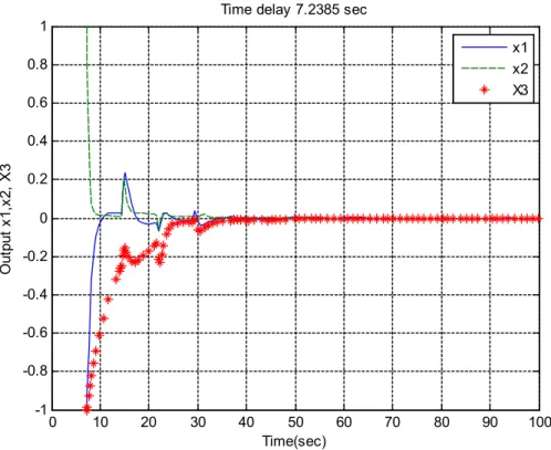
under different methods such that the system (31) is globally asymptotically stable. According to the Table 1, this example shows that the stability criterion in this paper gives much less conservative results than those in the literature [1, 8, 22, 35]. Fig. 1 shows the state response of example 1 withh 1 0and h27.2385, with
activation function T
1 2 1
( ( )) [0.02 tanh( ( )), 0.05 tanh( ( )),0.05 tanh( ( )), ] ,
g x x t x t x t when the
initial value is [ 1, 1, -1] T.
Example 2. Consider neutral-type neural networks with interval time-varying delays follows:
( ) ( ( )) ( ) ( ( )) ( ( ( ))),
where 2.7644 0 0 0.2651 -3.1608 -2.4687 0 1.0185 0 , 3.1859 -0.1573 0 , 0 0 10.2716 2.0368 -1.3633 0.5776 C A -0.7727 -0.8370 3.0819 0.2076 0.0631 0.3915 0.1004 0.6677 -2.4431 , -0.0780 0.3106 0.1009 . -0.6622 1.3109 -1.8407 -0.2763 0.1416 0.3729 B D
The neuron activation functions are assumed to satisfy Assumption 1 with {0.1019,0.3419,0.0633}.
K diag
Solution: Table 2 gives the comparison results on the maximum delay bound allowed via the methods in recent papers [1, 34, 40] and our new study. According to the Table 2, this example shows that the stability criterion in this paper can lead to less conservative results [1, 34, 40]. Therefore, the concerned neural networks with time delays (32) are asymptotically stable. Fig. 2 shows the state response of example 2 with h 1 0 and
2 22.0276,
h
T
1 2 1
( ( )) [0.02 tanh( ( )),0.05 tanh( ( )),0.05 tanh( ( )), ] ,
g x x t x t x t when the initial
value is [ 1, 1, -1] T.
Remark1: To obtain delay-derivative-dependent stability criteria, the double integral term
1 0 1 ( ) ( ) , t T t h x s Rx s dsd 1 1 ( ) 2 ( ) , t h T t h x s R x s dsd 1 2 ( ) 3 ( ) , t h T t h x s R x s dsd and 0 4 ( ) ( ) t T t x s R x s dsd
in LKF are widely used. When taking their derivative, they were
simply enlarged as 1 1 1 ( )( 1 33) ( ) , 1 ( )( 2 33) ( ) , 1 ( )( 2 33) ( ) , t T t h T t h T t h x s R X x s ds t h x s R Y x s ds t h x s R Y x s ds 1 2 ( )( 3 33) ( ) , t h T t h x s R Z x s ds and ( )( 4 33) ( ) . t T tx s R M x s ds
Then, we faced the key issue of reducing conservatism by dealing with these integral terms. In this regard, recently, many researchers have attempted to estimate its upper bounds with various techniques. Thus, to achieve this, we have utilized a new IIT in Theorem 1 to compute the new upper bounds of
such integral terms as 1 1
1 ( ) 33 ( ) , 1 ( ) 33 ( ) , 1 ( ) 33 ( ) , t T t h T t h T t h x s X x s ds t h x sY x s ds t h x sY x s ds 1 2 ( ) 33 ( ) , t h T t h x s Z x s ds and ( ) 33 ( ) t T tx s M x s ds
shown to be tighter than those of [1, 8, 22, 34, 35, 40].
5. Conclusions
In this paper, we have refined the delay-derivative-dependent stability analysis for neutral-type neural networks with interval time-varying delays. By combining delayed decomposition approach (DDA) and integral inequality approach (IIA), some improved delay-derivative-dependent criteria with less conservatism have been obtained. The delayed decomposition approach based LKFs lead to delay-derivative- dependent criteria that depend on both the upper and lower bounds on the delay derivative. The case when the derivative’s lower bound is unknown is also considered, as the case when no restrictions are cast upon the delay derivative. The new criteria are applicable to both fast and slow time-varying delays. The obtained conditions are derived in terms of LMIs which are easy to be verified by using various convex optimization techniques like an interior point method or software packages like MATLAB LMI Toolbox. Finally,two well-known examples show that these methods reduced conservatism and improved the maximum admissible upper bounds (MAUBs) of the time-delay.
References
[1]. Ali MS. Novel delay dependent stability analysis of Takagi Sugeno fuzzy uncertain neural networks with time varying delays. Chinese Physics B 2012; 21: 070207-1-12. [2]. Boyd S, Ghaoui LE, Feron E, Balakrishnan V. Linear Matrix Inequalities in System and
Control Theory. SIAM, Philadelphia, 1994.
[3]. Cao J, Yuan K, Li HX. Global asymptotical stability of recurrent neural networks with multiple discrete delays and distributed delays. IEEE Transactions on Neural Networks 2006; 17:1646-1651.
[4]. Chen B, Li H, Lin C, Zhou Q. Passivity analysis for uncertain neural networks with discrete and distributed time-varying delays. Physics Letters A 2009; 373: 1242-1248. [5]. Cheng CJ, Liao YL, Yan JY, Hwang CC. Globally asymptotic stability of a class of
neural-type neural networks with delays. IEEE Transactions on Systems Man and Cybernetics- Part B-Cybernetics 2006; 36:1191-1195.
[6]. Cheng L, Hou ZG, Tan M. A neutral-type delayed projection neural network for solving nonlinear variation inequalities. IEEE Transactions on Circuits and Systems II-Express Briefs 2008; 55: 806-810.
[8]. Feng J, Xu SY, Zou Y. Delay-dependent stability of neutral type neural networks with distributed delays. Neurocomputing 2009; 72:2576-2580.
[9]. He Y, Wu M, She JH, Liu GP. Parameter-dependent Lyapunov functional for stability of time-delay systems with polytopic-type uncertainties. IEEE Transactions on Automatic Control 49(2004) 828-832.
[10].Hua C, Long C, Guan X. New results on stability analysis of neural networks with time-varying delays. Physics Letters A 2006; 352:335-340.
[11].Li CD, Liao XF, Zhang R. Global robust asymptotical stability of multi-delayed interval neural networks: an LMI approach, Physics Letters A 2004; 328: 452-462.
[12].Li H, Chen B, Zhou Q, Qian W. Robust stability for uncertain delayed fuzzy Hopfield neural networks with Markovian jumping parameters. IEEE Transactions on Systems Man and Cybernetics- Part B-Cybernetics 2009; 39: 94- 102.
[13].Li T, Guo L, Sun C, Lin C. Further result on delay-dependent stability criterion of neural networks with time-varying delays. IEEE Transactions on Neural Networks 19(2008) 726-730.
[14].Li T, Guo L, Lin C. Stability criteria with less LMI variables for neural networks with time-varying delay. IEEE Transactions on Circuits and Systems II-Express Briefs 2008; 55:1188-1192.
[15].Li X, Fu X, Balasubramaniam P, Rakkiyappan R. Existence, uniqueness and stability analysis of recurrent neural networks with time delay in the leakage term under impulsive perturbations. Nonlinear Analysis: Real World Applications 2010; 11: 4092-4108.
[16].Liao C, Lu C. Passivity analysis for uncertain time-varying delayed neural networks with neutral type. In Second International Conference on Innovative Computing, Information and Control 2007, ICICIC’07, IEEE, 2007: 70-74.
[17].Liao TL, Yan JJ, Cheng C, Wang CC. Globally exponential stability condition of a class of neural networks with time-varying delays. Physics Letters A 2005; 339: 333-342. [18].Lien CH, Yu KW, Lin YF, Chung YJ, Chung LY. Global exponential stability for
uncertain delayed neural networks of neutral type with mixed time delays. IEEE Transactions on Systems Man and Cybernetics- Part B-Cybernetics 2008; 38:709-720. [19].Liu D, Hu S, Wang J. Global output convergence of a class of continuous-time recurrent
neural networks with time-varying thresholds. IEEE Transactions on Circuits and Systems II-Express Briefs 2004; 51:161-167.
cellular networks. IEEE Transactions on Neural Networks 2005; 16: 1219-1228.
[21].Liu PL. Improved delay-dependent robust stability criteria for recurrent neural networks with time-varying delays. ISA Transactions 2013;52(1):30-35.
[22].Liu PL. Improved delay-dependent stability of neutral type neural networks with distributed delays. ISA Transactions 2013; 52(6):717-724.
[23].Liu PL. New results on delay-range-dependent stability analysis for interval time-varying delay systems with non-linear perturbations, ISA Transactions 2015; 57: 93-100.
[24].Park JH, Kwon OM, Lee SM. LMI optimization approach on stability for delayed neural networks of neutral-type. Applied Mathematics and Computation 2008; 196:236-244. [25]. Park JH, Kwon OM. Further results on state estimation for neural networks of
neutral-type with time-varying delay. Applied Mathematics and Computation 2009; 208: 69-75.
[26]. Rakkiyappan R, Balasubramaniam P. Delay-dependent asymptotic stability for stochastic delayed recurrent neural networks with time varying delays. Applied Mathematics and Computation 2008;198: 526-533.
[27].Shao HY. Delay-dependent stability for recurrent neural networks with time-varying delays. IEEE Transactions on Neural Networks 2008; 19 (9):1647-1651.
[28].Tong SC, Li YM, Zhang HG. Adaptive neural network decentralized backstepping output-feedback control for nonlinear large-scale systems with time delays. IEEE Transactions on Neural Networks 2011;22(7):1073-1086.
[29].Tong SC, Wang T, Li YM, Zhang HG. Adaptive neural network output feedback control for stochastic nonlinear systems with unknown dead-zone and unmodeled dynamics. IEEE Transactions on Cybernetics 2014;44(6):910-921.
[30].Wang W, Cao JD. LMI-based criteria for globally robust stability of delayed Cohen-Grossberg neural networks. IEE Proceedings Control Theory & Applications 2006; 153: 397-402.
[31].Wu M, He Y, She JH. New delay-dependent stability criteria and stabilizing method for neutral systems. IEEE Transactions on Automatic Control 2004; 4: 2266-2271.
[32].Wu M, Cui BT, Lou XY. Some criteria for asymptotic stability of Cohen- Grossberg neural networks with time-varying delays. Neurocomputing 2007; 70: 1085-1088. [33].Wu M, Liu F, Shi P, He Y, Yokoyama R. Exponential stability analysis for neural
networks with time-varying delay. IEEE Transactions on Systems Man and Cybernetics-Part B-Cybernetics 2008; 38: 1152-1156.
[34].Xu S, Lam J, Ho DWC, Zou Y. Delay-dependent exponential stability for a class of neural networks with time delays. Journal of Computational & Applied Mathematics 2005; 183:16-28.
[35].Xu S, Lam J, Ho DWC. Novel global robust stability criteria for interval neural networks with multiple time-varying delays. Physics Letters A 2005; 342: 322-330. [36].Yu GJ, Lu CY, Tsai JSH, Liu BD, Su TJ. Stability of cellular neural networks with
time-varying delay. IEEE Transactions on Circuits and Systems I, Fundamental Theory Applications 2003; 50:677-678.
[37].Yu W, Li X. Some stability properties of dynamic neural networks. IEEE Transactions on Circuits and Systems I, Fundamental Theory Applications 2001; 48: 256-259.
[38].Zhang H, Wang Z, Liu D. Robust exponential stability of recurrent neural networks with multiple time-varying delays. IEEE Transactions on Circuits and Systems II-Express Briefs 2007; 54:730-734.
[39].Zhang H, Wang Z, Liu D. Global asymptotic stability of recurrent neural networks with multiple time-varying delays. IEEE Transactions on Neural Networks 2008; 19:855-873. [40].Zuo Z, Wang Y. Novel delay-dependent exponential stability analysis for a class of
delayed neural networks. Lecture Notes in Computer Science 2006; 4113: 216-226. [41].Zuo ZQ, Yang C, Wang Y. a new method for stability analysis of recurrent neural
networks with interval time-varying delay. IEEE Transactions on Neural Networks 2010; 21(2)339-344.
Table 1
Comparisons of the MADB h in Example 1
Method Xu et al. [35] Feng et. al. [8] Ali [1] Liu [22] Liu [23] Theorem 1
h 0.2321 1.8545 2.0990 4.9985 6.9874 7.2835
Table 2
Comparisons of maximum allowable delay bound (MADB) h in Example 2
Method Xu et al. [34] Zuo and Wang [43] Ali [1] Liu [23] Theorem 1
![[2015-Fall] WNFA lab1 - CamCom](data:image/gif;base64,R0lGODlhAQABAIAAAP///wAAACH5BAEAAAAALAAAAAABAAEAAAICRAEAOw==)