太平洋年代際震盪對雲與輻射效應之影響：氣候模式之評估與診斷

國立臺灣大學理學院大氣科學研究所 碩士論文

Graduate Institute of Atmospheric Sciences College of Science

National Taiwan University Master thesis

太平洋年代際震盪對雲與輻射效應之影響：

氣候模式之評估與診斷

Cloud and Radiative Balance Changes in Response to Inter- Decadal Pacific Oscillation: Global Climate Model

Diagnostics and Evaluation

陳勇志 Yong-Jhih Chen

指導教授：黃彥婷博士 Advisor: Yen-Ting Hwang, Ph.D.

中華民國 105 年 7 月

July, 2016

ii

中文摘要

本研究之目標在於探討太平洋年代際震盪對雲之影響，並估計在衛星觀測紀 錄中，太平洋年代際震盪對雲量之長期趨勢的貢獻。在過去的三十年間，衛星技術 的成熟使雲量觀測的可信度大幅提高。然而，在這段期間，太平洋年代際震盪的相 位有相當明顯的轉變，對整個氣候系統有顯著的影響。這代表在過去觀測到的雲量 趨勢，除了受到全球暖化、火山以及氣膠等外在作用力影響之外，亦可能包含了太 平洋年代際震盪相位轉變的訊號。理解太平洋年代際震盪與雲之關聯，有助於我們 更清楚地解釋觀測到的雲量趨勢。

我們使用了四個在全球暖化下，雲的表現最不同的氣候模式進行分析。在這 些模式中，太平洋年代際震盪和雲的關聯非常相似，並和觀測的推估吻合。藉助氣 候模式，我們估計在觀測期間，太平洋年代際震盪的相位轉變對於雲量趨勢的貢 獻。結果顯示，和太平洋年代際震盪有關的雲量趨勢和衛星觀測之雲量的長期趨 勢：一、就區域分佈而言，兩者在太平洋上的很多區域都有一致的趨勢；二、就量 值而言，兩者大約在同一個數量級，顯示自然震盪對雲量趨勢的影響是不可忽略 的。

關鍵字：雲回饋，太平洋年代際震盪，全球暖化，大尺度環流，衛星觀測

Abstract

The goal of this study is to investigate the cloud responses to Inter-decadal Pacific Oscillation (IPO), and estimate how IPO contributes to the observed cloud cover trend. In the past 30 years, the reliability of observational cloud data has been largely improved by satellite measurement. During this period, in addition to the background warming of global mean surface temperature, a phase shift of IPO had also occurred, introducing changes in sea surface temperature, large-scale circulations and clouds. A better understanding of cloud changes associated with IPO may be helpful for understanding the variability of clouds in satellite records.

We investigated the IPO-related cloud changes in four global climate models (GCMs) that have the most different global mean cloud feedbacks under global warming.

All of the models simulate similar IPO-related cloud changes that are consistent with observations. The contribution of IPO to observed cloud cover trend is estimated, and the magnitude is comparable to the cloud cover trend in observation. When comparing to the global warming related cloud cover trend, there are indications that the IPO and global warming may both contribute to the observed cloud cover trend in a few regions: (1) the reduction of cloud cover in the mid-latitude northwest/southwest Pacific between 30~40⁰N/S, and (2) a positive trend between 5⁰N~20⁰S and a negative trend between 25~40⁰S in the eastern Pacific. In some other regions, such as the northeast Pacific, the IPO and global warming may have the opposite contributions to the observed cloud cover trend.

Our results suggest the influence of IPO may be important to the cloud cover trend

iv

Key words: Cloud feedback, Inter-Decadal Pacific Oscillation, global warming, large-scale circulation, satellite observation

Contents

口試委員審定書 ... i

中文摘要 ... ii

Abstract ... iii

Contents ... v

List of Figures ... vii

List of Tables ... x

Chapter 1. Introduction ... 1

1.1 The cloud cover trend: external forcing and internal variability ... 1

1.2 IPO and clouds ... 2

1.3 Global warming and clouds ... 4

1.4 The scope of the study ... 5

Chapter 2. Data and Methods ... 6

2.1 Data ... 6

2.1.1 Observation and reanalysis datasets ... 6

2.1.2 Models and experiments ... 6

2.2 Methods ... 8

vi

2.2.3 The monthly regression relationships and the multiple regression relationships ... 10

Chapter 3. Cloud Changes: IPO and Global Warming ... 12

3.1 IPO-related anomalies of large-scale fields and clouds ... 12

3.1.1 Large-scale fields ... 12

3.1.2 The cloud responses and the relationships with large-scale fields ... 14

3.1.3 Estimating biases of the model ... 17

3.2 Changes of Large-scale fields and clouds under global warming ... 20

Chapter 4. Conclusions and discussions ... 22

4.1 IPO and global warming in GCMs ... 22

4.2 IPO and global warming fingerprints in the observed cloud cover trend ... 24

Reference ... 27

Tables ... 32

Figures ... 34

Appendix ... 43

List of Figures

Fig. 1.1: Anomaly patterns associated with a +1 standard deviation departure of the IPO Index in observation. a. SST from HadISST, b. vertical motion (omega) at 500 hPa from ERA-40 (positive downward), c. vertical motion (omega) at 500 hPa from ERA-Interim (positive downward). ... 34 Fig. 3.1: Anomaly patterns associated with a +1 standard deviation departure of the IPO

Index in CESM. a. SST (shading) and its climatology (contours), b. vertical motion at 500 hPa (shading) and its climatology (contours), c. geopotential height at 300 hPa (shading) and surface pressure (contours), the contour interval is 0.1 hPa, d. near-surface meridional wind (shading) and SST (contours), the contour interval is 0.1⁰C. Contours with negative values are dashed. The dots in (a) and (b) indicate all models agree on the sign of the anomalies. ... 35 Fig. 3.2: Anomaly patterns associated with a +1 standard deviation departure of the IPO

Index in CESM. a. total cloud fraction (shading) and its climatology (contours), b.

high cloud fraction (shading) and vertical motion at 500 hPa (contours), the

contour interval is 1 hPa/day, c. Low cloud fraction (shading) and SST-related low cloud anomaly (contours), the contour interval is 0.2%, and d. SW CRE e. LW CRE f. net CRE. Contours in (b) and (c) with negative values are dashed. The dots in (a), (d), (e) and (f) indicate all models agree on the sign of the anomalies. ... 36 Fig. 3.3: The monthly regression relationship between net CRE and SST in a. CESM and b.

viii

Fig. 3.4: The multiple regression relationship between SW CRE and large-scale fields. a, b The SST coefficient in a. CESM and b. observation, and c, d the vertical motion coefficient in c. CESM and d. observation. ... 38 Fig. 3.5: The SW CRE anomalies during IPO estimated by SST and vertical motion, in a.

CESM and b. observation. The estimation is computed by summing the product of the IPO-related anomalies of SST/vertical motion (Fig. 3.1a, 3.1b for CESM and Fig. 1a, 1c for observation) and the corresponding SST/vertical motion coefficient in multiple regression relationships (Fig. 3.4a, 3.4c for CESM and Fig. 3.4b, 3.4d for observation). See Chapter 2.2.3 for the detailed calculation. ... 39 Fig. 3.6: The multi-model mean of anomaly patterns associated with 1K warming of global

mean surface temperature. a. SST, b. vertical motion at 500 hPa, c. total cloud fraction and d. SW CRE e. LW CRE f. net CRE. The dots in (b)-(f) indicate all models agree on the sign of the anomalies. ... 40 Fig. 4.1: The estimation of a. IPO contribution, and b. global warming contribution to the

observed cloud cover trend. c. Locations where IPO and global warming agree on the sign of anomalies. Green/brown indicates the IPO and global warming both contribute to an increasing/decreasing of cloud. The dots in (a), (b) indicate all models agree on the sign of the anomalies, and dots in (c) indicate all models agree on the sign of the anomalies in IPO and global warming. ... 41 Fig. 4.2: Figure. 1 in Norris et al. (2016). a. Trend in average of PATMOS-x and ISCCP

total cloud amount 1983–2009. b. Change in albedo from January 1985–December 1989 (ERBS) to July 2002–June 2014 (CERES). c. Trend in ensemble mean total cloud amount 1983–2009 from CMIP5 historical simulations with all radiative

forcings (ALL). d. Locations where majority of observations and majority of simulations show increases (blue) or decreases (orange). Black dots indicate agreement among all three satellite records on sign of change in (a) and (b) and trend statistical significance (P < 0.05 two-sided) in c. All trends and changes are relative to the 60° S–60° N mean change. ... 42

x

List of Tables

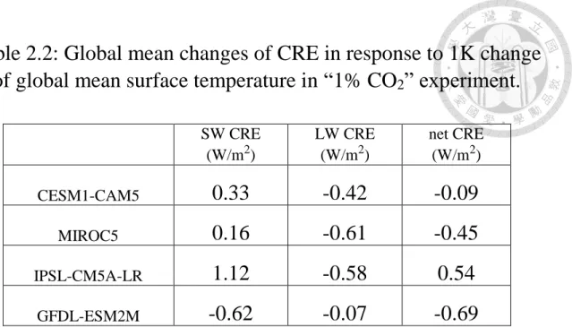
Table 2.1: Models used in this study. ... 32 Table 2.2: Changes of global mean CRE in response to 1K change of global mean

surface temperature in 1% “CO2” experiment. ... 33 Table 3.1: Changes of global mean surface temperature and CRE in response to a +1

standard deviation departure of the IPO Index ... 33

Chapter 1. Introduction

1.1 The cloud cover trend: external forcing and internal variability

Clouds can influence top of atmosphere (TOA) energy budget through their radiative effects and hence impact the climate system. The disagreement of the future projections between global climate models (GCMs) is mostly due to the diversity of clouds and the accompanied radiative effects (Andrews et al. 2012; Bellomo et al. 2014). Bony and Dufresne (2005) proposed that it is the marine boundary layer clouds that contribute to most of the inter-model spread of cloud radiative effects. Given the large uncertainty and strong impacts of clouds, understanding the response of clouds to global warming is critical for future projections.

Since the beginning of the satellite record in 1979, the reliability of observational clouds data had improved significantly (Schiffer and Rossow 1983). The observation, aside from climate models, provides another way to estimate the cloud responses to

anthropogenic forcing. However, in addition to external forcing, the observed cloud cover trend may also be influenced by low-frequency internal variability which has comparable timescale with the satellite records. Based on the observed sea surface temperature (SST) in the 20^th century, the top three dominant modes of low-frequency variations include global warming, Inter-decadal Pacific Oscillation (IPO) and Atlantic Multi-decadal Oscillation (AMO), explaining about 56%, 10% and 8% of low-frequency SST variation, respectively (Parker et al. 2007). During the satellite era, in addition to the raising of global mean

2

in Pacific (Trenberth et al. 2014), suggesting that changes of climate system during satellite era may be also largely influenced by IPO. As external forcing and internal variability both contribute to the observed cloud cover trend, a better understanding of cloud changes associated with IPO, which represents the most important internal variability over the Pacific basin, may be helpful for understanding the observed trend of cloud cover.

In previous literature, the relationship between IPO and clouds had not yet been explored thoroughly, due to limited time and spatial converge of cloud observations. In this study, we investigate the cloud responses to IPO and global warming by GCM simulations, and the cloud responses to IPO will be investigated in detail. We will further estimate that, given the phase switch of IPO and the anthropogenic warming trend observed during satellite era, how will IPO and global warming contribute to the observed cloud cover trend.

1.2 IPO and clouds

The IPO is the dominant decadal time scale SST variation over the Pacific basin. It is characterized by an ENSO-like SST pattern, but with the magnitude of SST anomaly in the tropics comparable with which in mid-latitudes (Dong and Dai 2015; Mantua et al.

1997; Newman et al. 2015). The IPO can influence climate in nearby area (Dai 2013;

Newman et al. 2015), and have global impacts on the climate system (Dong and Dai 2015).

Throughout the past 100 years, IPO accounts for most of the observed discrepancy in global mean temperature from the anthropogenically forced climate response (Kosaka and Xie 2013). The global mean surface temperature has much smaller trend after 1998,

when the phase change of IPO occurs. Moreover, the SST difference before and after 1998 is very IPO-like, and the geopotential height at 300 hPa also exhibits wave-like pattern triggered in the tropical central Pacific and propagating poleward, which coincident with the character of IPO, suggesting an IPO impact on climate system (Trenberth et al. 2014).

England et al. (2014) shows that the strengthening in Pacific trade winds accompanied by the phase shift of IPO increases the ocean heat uptake, and result in the global warming hiatus in past two decades.

Despite limited time and spatial converge, there are a few observational evidence demonstrating the influence of IPO on clouds. Using Synoptic Cloud Reports Archive from ships, Norris (2000) shows that, in the northern Pacific, the decadal variation of storm tracks, nimbostratus frequency and marine stratiform cloudiness is significantly correlated with the decadal variation of SST. In Clement et al. (2009), cloud fraction observed by satellite (International Satellite Cloud Climatology Project, ISCCP) is regressed on smoothed area mean SST in subtropical Northeast Pacific, which is correlated with IPO.

The result suggests, during positive phase of IPO, cloud fraction decreases in Maritime Continent and stratocumulus zone in the eastern Pacific, and increases in the tropical western Pacific and the tropical central Pacific.

However, it is challenging to obtain an accurate global view for the cloud changes associated with IPO using the limited length of satellite observation. The GCMs, on the other hand, are complimentary tools for investigating the problem, as they can provide pure natural variability signal by experimental design, and are able to generate unlimited length

4

1.3 Global warming and clouds

The global warming is the increase in Earth’s average surface temperature due to anthropogenic emission of green-house gases (Eickemeier et al. 2014; Lashof and Ahuja 1990). The global warming can largely influence the general circulation and hydrological cycle, and has great impact on global climate (Bengtsson, Hodges, and Roeckner 2006;

Held and Soden 2006; Lau and Kim 2015; Marvel et al. 2015).

In previous studies, some robust characters about how climate system responds to global warming are investigated. Chang et al. (2012) showed the storm track will shift poleward under global warming. Lau and Kim (2015) demonstrated that, the global warming is accompanied by the strengthening and narrowing of deep-tropics, the

weakening subsidence in the subtropics, and the expansion of Hadley cell in mid-latitude.

Marvel et al. (2015) investigated the latitude where the maximum and minimum of zonal mean total cloud fraction locates, and found that under global warming, the latitude of maximum and minimum zonal mean total cloud fraction will shift poleward, the height of high cloud in these latitude will rise, and the cloud fraction increases (decreases) in the latitude of maximum (minimum) zonal mean total cloud fraction.

Despite these robust features under global warming, the global mean of net cloud radiative effect (CRE) is very different across models, contributes to most of the

uncertainty in climate sensitivity (Andrews et al. 2012). The inter-model spread of net CRE is mostly contributed by the marine boundary layer clouds (Bony and Dufresne 2005;

Zelinka et al. 2013). Bellomo et al. (2014) further investigated several regions with larger

cloud amount feedback, which represents the changes of CRE due to cloud fraction

changes, in the period of 1954~2005 in observation and CMIP5 historical simulations, and found large disagreement between models. The CREs behavior can be different between models, even when the cloud cover responses are consistent.

1.4 The scope of the study

The goal of this study is to investigate the relationships between clouds and IPO, and estimate how IPO contributes to the observed cloud cover trend. To reach this goal, we first analyze the 500-year pre-industrial GCM simulations to construct a thorough

understanding of the large-scale fields and the cloud changes associated with IPO. The relationships between clouds and large-scale fields are examined (Chapter 3.1). The global warming impacts on clouds are investigated to compare with those of IPO (Chapter 3.2).

We then estimate the contributions of IPO-related and global warming related cloud changes in satellite observation, using reanalysis and observational data (Chapter 4).

We attempt to address the following questions: How do clouds respond to IPO?

How important is the IPO-related cloud cover trend in observation? What is the relative contribution of IPO and global warming to the cloud cover trend observed by satellite?

How do we make use of observational data to evaluate the reliability of GCMs?

6

Chapter 2. Data and Methods

2.1 Data

2.1.1 Observation and reanalysis datasets

Some observational and reanalysis datasets are used in this study to compare with the GCM simulations. The SST data is obtained from the Hadley Centre Global Sea Ice and Sea Surface Temperature (HadISST, Rayner et al. 2003) dataset of Hadley Center. The HadISST is a dataset of globally SST and sea ice concentration on 1⁰×1⁰ latitude/longitude grid from 1870 to present, in this study the period of 1920~2013 is analyzed to obtain the IPO index. The HadISST mainly uses ship observation data before 1982, and since then the satellite-derived SSTs had been included. The vertical motion data is obtained from two reanalysis datasets of European Centre for Medium-Range Weather Forecasts (ECMWF), the ERA40 (1957~2002, Uppala et al. 2005) and ERA-Interim (1979~2013, Dee et al.

2011), generated by assimilating satellite, surface, radiosonde and pilot observations. The CREs data is obtained from the Clouds and the Earth's Radiant Energy System (CERES, Wielicki et al. 1996),a satellite observation dataset of TOA radiation fluxes of National Aeronautics and Space Administration (NASA), and the period of 2000~2010 is analyzed.

2.1.2 Models and experiments

In this study, we analyze four GCMs to investigate the cloud changes during IPO and global warming: CESM1-CAM5, MIROC5, IPSL-CM5A-LR and GFDL-ESM2M (Table 2.1). The MIROC5 and the IPSL-CM5A-LR, according to Andrews et al. (2012), are the two models with most different global mean cloud feedback in the “abrupt

quadruple CO2” experiment, in which the CO2 concentration is quadrupled abruptly. The CESM1-CAM5 and GFDL-ESM2M are chosen because of some historical reasons.

Stephens 2005 showed that, in NCAR CAM2 and GFDL-AM2, which are formal versions of CESM-CAM5 and GFDL-ESM2M, the low cloud responses to greenhouse gas forcing are very different, with the opposite signs almost globally. The global mean cloud

feedbacks of the four GCMs are listed in Table 2.2.

We make use of the “pre-industrial” experiments in CMIP5 to get the unforced and intrinsic characteristics of IPO. In the “pre-industrial” experiment, the external forcing and land use are fixed to the pre-industrial condition, and the simulations continue for

thousands of years. Here we analyze 500 years of outputs in each model. For CESM1- CAM5, the data of “pre-industrial” is taken from the pre-industrial control run of BGC-LE (Bio-Geo-Chemistry Large Ensemble) experiment of NCAR rather than from the CMIP5 archive, because in CMIP5 the CESM only provide 320 years of pre-industrial simulation.

The difference between pre-industrial simulation in BGC-LE and CMIP5 is the Bio-Geo- Chemistry process in BGC-LE experiment. Comparison of the IPO-related anomalous fields between the two experiments show the difference has negligible effects to our results.

To obtain the responses of clouds to greenhouse gas forcing, the “1% CO2” experiment in CMIP5 is diagnosed, which is initialized from the “pre-industrial”

experiment and hold everything unchanged except for the CO2 concentration, which is increased by 1% every year. We analyze the first 140 years of the simulations, during which the CO2 concentration quadrupled.

8

2.2 Methods

In this section, some methodologies used in this study are introduced. To obtain the signals of IPO and global warming, the empirical orthogonal function (EOF) analysis is applied. In section 2.2.1 we briefly introduce the EOF analysis, and the diagnostics of IPO and global warming signal are described in section 2.2.2. To investigate the relationships between clouds and large-scale fields, the linear regression analysis is applied to obtain the monthly regression relationships, which are explained in section 2.2.3.

2.2.1 The Empirical orthogonal function analysis

The EOF analysis is a statistical approach commonly used in climate diagnostics.

The concept of EOF analysis is to decompose the data into orthogonal spatial patterns called EOF patterns or EOF modes, and maximize the inhomogeneity of variance explained by each pattern. By doing so, the patterns that can better describe the characteristics of the variations of the data will be highlighted. Each EOF pattern is accompanied by a time series called principle component (PC), which is the projection of the data on the EOF mode. In this study, EOF analysis is applied on SST to obtain the pattern that best explain the SST variation.

2.2.2 The diagnostics of IPO and global warming signal

Traditionally, the IPO is defined as the dominant mode of SST in the Pacific basin after the effect of anthropogenic forcing is removed from data and the high-frequency variability is smoothed out. During the past century, the anthropogenic climate change

dominants the observed variability, the leading EOF mode represents the global warming mode, and the IPO is then defined as the second EOF mode (Dai 2013; Dong and Dai 2015;

Parker et al. 2007).

In this study, we diagnose the CMIP5 “pre-industrial” simulations. Since the SST is not influenced by external forcing due to experimental design, the IPO is defined as the leading EOF mode of SST in Pacific basin, after a 13 year low-pass filter via fast Fourier transform algorithm is applied on the GCM outputs to remove high-frequency variations.

Variables are then regressed on the PC of leading EOF mode to obtain corresponding anomalous field of one standard deviation change in PC, the IPO index. In observation, the IPO is defined as the second EOF mode of global SST from 1920 to 2013, after a 13 year low-pass filter is applied on SST data. The vertical motion is then regressed on the corresponding PC to obtain corresponding anomalous field of one standard deviation change in PC.

The influence of global warming on large-scale fields and clouds is investigated in the CMIP5 “1% CO2” simulations. The EOF analysis is applied on global SST, and the leading EOF mode represents the global warming response, the correlation coefficient of the corresponding PC and global mean surface temperature is above 0.99 in all model after the PC is rescaled so that unit change in PC corresponding to one degree change of global mean temperature. Variables are then linearly regressed on the rescaled PC at each grid point to obtain the anomaly per degree change of global mean temperature.

10

2.2.3 The monthly regression relationships and the multiple regression relationships

To investigate how cloud changes are related to variation of local SST or vertical motion on monthly time scale, a simple linear regression is applied. In this study, the monthly regression relationship refers to the linear regression between two monthly mean variables at each grid point, after the seasonal cycle is removed:

Cloud properties = ∝ × L + constant + error , where L is the large-scale variable, can be either SST or vertical motion at 500 hPa. The ∝ is the slope of the regression line of cloud properties and large-scale variables, obtained by minimizing the mean square error.

The purpose is to find the local relationship between large-scale fields and clouds.

By a simple linear regression, we can obtain the cloud anomaly accompanied by unit anomaly of SST or vertical motion departure from its climatology seasonal cycle at each grid point.

We examine the monthly regression relationship between clouds and large-scale fields in CMIP5 “pre-industrial” simulations and in observation. In “pre-industrial”

simulations, the linear regression is applied to the whole 500 years. In observation the linear regression is applied to the period of 2000~2010, when the CERES CREs data is available. To test whether the difference of monthly regression relationships between GCMs and observation are arise due to the unequal data length, the 500-year-long data of GCMs is cut into a set of 10-year-long chunks. The monthly regression relationships in each 10-year-long chunk (not shown) are roughly agree with those of the 500-year-long

data, suggest that the observation data is long enough to capture the feature of monthly regression relationships.

The multiple regression relationship is generated by multiple linear regression method, and is same as monthly regression relationship except for it has two independent variables: SST and vertical motion at 500 hPa, instead of one of them in the case of monthly regression relationship:

Cloud properties = ∝ × T + β × 𝜔₅₀₀+ constant + error, where the T and 𝜔₅₀₀ are the anomalies of SST and vertical motion at 500 hPa. The ∝ and β, which are called the SST coefficient and vertical motion coefficient in this study, respectively, obtained by minimizing the mean square error. The purpose is to combine the effect from SST and vertical motion.

12

Chapter 3. Cloud Changes: IPO and Global Warming

3.1 IPO-related anomalies of large-scale fields and clouds

3.1.1 Large-scale fields

To set the stage for investigating the relationship between clouds and large-scale fields in Chapter 3.1.2, we first present the SST and circulation anomalies associated with IPO in GCMs. We also evaluate GCMs’ ability to simulate IPO by comparing with reanalysis and observational data.

The IPO-related changes of SST, vertical motion at 500 hPa, clouds and CRE are diagnosed in four GCMs. In the CESM, high and low cloud responses are further

investigated. In this chapter, we will show our results in CESM, and dot the regions that all models agree in sign. By presenting the results of one model instead of multi-model mean, we can demonstrate the linkage between IPO-related anomalies and climatology more clearly, since the climatological large-scale fields may be different across models. The climatological conditions and the IPO-related anomalous fields in other models are shown in Figure A1.

The SST pattern of IPO is similar to ENSO but with broader spatial scale (Fig. 1.1a, Fig. 3.1a). Its positive phase is accompanied by anomalous warm SST in the tropical Pacific, with maximum located in the central Pacific region. In the extra-tropics, SST anomaly is characterized by a dipole structure, with cold anomaly in the western Pacific and warm anomaly in the eastern Pacific. The minimum of SST anomaly locates at mid- latitude central Pacific (~180⁰W in the northern Pacific, ~130⁰W in the southern Pacific).

The surface pressure anomalies exhibit a wave-like pattern, with anomalous low pressures in mid-latitudes of both hemispheres, and an increased zonal pressure gradient in the tropics. In the geopotential height at 300hPa (Fig. 3.1c), the main features are the highs locating at both side of the equator, and a wave-train pattern propagating poleward and deepening the Aleutian low in North Pacific. The vertical motion at 500 hPa (Fig. 1.1b, c, Fig. 3.1b) shows an enhancement of ascending motion in the tropical western Pacific and equatorial shift of Intertropical Convergence Zone (ITCZ) andSouth Pacific Convergence Zone (SPCZ). In Northwest Pacific, the subtropical subsidence zone weakens and expands into mid-latitudes. In Southwest Pacific the subsidence is enhanced. In the eastern Pacific, the subsidence weakens between 15~40⁰N/S. The meridional wind at lowest model level (about 60m above sea level) shows there is equatorward flow in the western Pacific and poleward flow in the eastern Pacific.

Figure 3.1a and Figure 3.1b show that the dynamical fields are tightly-coupled to SST. The wave-train pattern in upper level geopotential height (Fig. 3.1c), along with the coincident pattern of the anomalous geopotential height at 300 hPa and surface pressure, suggests a “teleconnection” between tropical SST and the low pressure centers in mid- latitudes of both hemispheres. The stationary wave teleconnection mechanism is consistent with those described in previous literature (Liu and Alexander 2007; Trenberth et al. 2014;

Zhang et al. 2016). The geotropic flow accompanied by the low sea level pressure brings cold and dry high-latitude air to the mid-latitude central Pacific, and brings warm and humid low-latitude air to the mid-latitude eastern Pacific, along the west coasts of North

14

wind in mid-latitude, and drives anomalous equatorward Ekman flow in the ocean, contribute to cooling in the central Pacific (Alexander and Scott 2008; Alexander et al.

2002; Newman et al. 2015).

In the western Pacific and the southern central Pacific, the pattern of vertical motion anomaly coincident with which of SST, with anomalous ascending (descending)

corresponding to anomalous warm (cool) SST. The ascending motion in the tropical western Pacific is largely enhanced due to the latent heat released by convection. In the eastern Pacific, the anomalous ascending motion in mid-latitude may be, by quasi- geostrophic balance, induced by the low level warm advection (Fig. 3.1d), which is initiated by the anomalous low pressure in mid-latitude central Pacific.

In summary, during the positive phase of IPO, the tropical central Pacific is anomalously warm, triggering the low-pressure anomaly in mid-latitude of both

hemispheres through teleconnection. The lows influence mid-latitude SST by horizontal advection, shaping the dipole structure. The SST then drives vertical motion.

The SST and circulation changes during IPO are robust across GCMs and are in good agreement with observation and reanalysis data (Fig. 1.1, Fig. 3.1a, 3.1b). This suggests that GCMs can simulate dominating processes for IPO development.

3.1.2 The cloud responses and the relationships with large-scale

fields

In this section, we investigate how clouds respond to IPO and the associated radiative effects. Fig. 3.2a demonstrates the anomalous total cloud fraction associated with the positive phase of IPO. In the deep tropical Pacific region, clouds increase over the warm pool region, around the western and central Pacific. The band of increasing clouds extends south and east, to the southern subtropical Pacific region. In the stratocumulus zone of Northeast Pacific and Southeast Pacific along the coast of America, the cloud fraction decreases.

In some regions, the high clouds (above 400 hPa, Fig.3.2b) and low clouds (below 700 hPa, Fig.3.2c) behave differently. In the tropical western and the tropical central Pacific, high cloud cover is largely increased and low cloud cover is slightly decreased, resulting in increased total cloud cover. In 20~40⁰N in the western and central Pacific, the high cloud cover decreases and low cloud cover increases, with overall increased total cloud cover in 20~30⁰N and decreased total cloud cover in 30~40⁰N. In the subtropical eastern Pacific (20~40⁰ in both hemispheres), the high cloud cover increases and low cloud cover decreases, resulting in an decreasing of total cloud cover in Northern Hemisphere and near zero change of total cloud cover in Southern Hemisphere.

The changes in clouds are tightly-coupled to the changes of large-scale fields. The pattern of high cloud fraction changes (Fig. 3.2b) coincident with which of vertical motion at 500 hPa, with ascending motion corresponding to more high clouds. A physical

explanation is, the vertical motion represents the occurrence of convection and provides upward moister flux, therefore is in good agreement with high cloud fraction. The low

16

the changes of SST, which has a strong control on the boundary layer’s static stability. The influence from SST change is estimated by multiplying the IPO-related SST anomaly (Fig.

3.1a) by the monthly regression relationship between low clouds and SST (Fig. 3.3a).

The patterns of cloud radiative effects (Fig. 3.2d-f) are consistent with which of cloud fraction anomalies, with the SW CRE corresponding to the total cloud fraction, the LW CRE corresponding to the high cloud fraction, and the net CRE corresponding to the low cloud fraction. When the total cloud fraction decreases (increases), there will be less (more) reflected solar radiation and a positive (negative) SW CRE anomaly. For the case of LW CRE, the higher clouds emit less outgoing LW radiation, thus keep more energy in the climate system. Increased high cloud fraction reduces outgoing LW radiation and lead to positive LW CRE anomaly. The net CRE is the summation of SW and LW CRE. For high clouds, it reflects incoming solar radiation and generates negative SW radiative effect, but it also emits less outgoing LW and generates positive LW radiative effect. Therefore, the SW and LW radiative effects from high clouds tend to cancel each other and have little contribution to net CRE. In the case of low clouds, the effect of LW warming is weak due to higher cloud-top temperature, and the SW cooling effect related with solar radiation reflection is much stronger. As a result, the net CRE is mainly contributed by the SW radiative effect of low clouds. Despite significant contribution for top-of atmosphere (TOA) fluxes in various regions, the global mean of net CRE is small, indicating the changes of clouds have little effect on global energy budget (Table 3.1).

Change in net CRE (Fig. 3.2f) shows that, due to cloud changes, there are

anomalously positive TOA fluxes in the eastern Pacific and the tropical central Pacific, and anomalously negative TOA fluxes in the western Pacific and the mid-latitude central

Pacific. The SW and LW CRE exhibit different effects on the climate system. The anomalous LW CRE is related with higher cloud trapping more LW energy, so the

anomalous LW CRE mostly represent the heating or cooling in the atmosphere, especially at the level of cloud top. The LW CRE in the atmosphere can change static stability and horizontal temperature gradient, and have potential influence on circulations (Li et al.

2015). The anomalous SW CRE is associated with the variations in cloud cover and their reflective solar radiation. The anomalous SW CRE has a direct influence on the oceanic surface, since the atmosphere absorbs little SW radiation. In the extra-tropics, the SW CRE (Fig. 3.2d) shows a warming effect in the eastern Pacific and cooling effect in the western Pacific, representing a positive feedback to local SST. This is consistent with the positive SST-low clouds feedback evidenced in Clement et al. (2009), in which the observed low cloud amount and local SST in the subtropical Northeast Pacific stratocumulus zone were analyzed. The warm SST reduces the low troposphere stability, making the splinter of stratocumulus and allowing more penetrating SW radiation to further heat the ocean surface. To understand how the LW and SW CRE then influence the structure or timescale of IPO, further GCM experiments may be necessary.

3.1.3 Estimating biases of the model

In this section, we estimate the possible model biases by comparing the monthly regression relationships in CESM and observation. The monthly regression relationships in other models are attached in Appendix A2. In GCMs, the cloud responses to IPO can be

18

relationships between clouds and large-scale fields. This approach allows us to qualitatively estimate the biases of models, by comparing the large-scale fields changes during IPO and the monthly regression relationships between clouds and large-scale fields in observation and in model simulations. Assuming cloud response linearly with small perturbation of large-scale environment within relatively short timescale, we use the monthly regression relationships obtained by inter-annual variations in the 10-year observational time period to understand the inter-decadal variability of clouds. Without such approach, hundreds years of cloud observation is needed to diagnose the IPO-related cloud changes in the real world.

Note, however, with the linear assumption, we can only perform qualitative comparison between observations and GCMs.

As the IPO-related anomalous patterns of large-scale fields are similar in

observation and in CESM (Fig. 1, Fig. 3.1), the biases are likely contributed primary by the monthly regression relationships betweenlarge-scale fields and clouds. The monthly regression relationships between CREs and large-scale fields in CESM is compared to which in observational data to investigate the potential biases in SW, LW and net CREs.

Since the IPO-related anomalous patterns of CREs are in good agreement with which of clouds, the biases in SW, LW and net CREs also reflect the biases in total cloud cover, high cloud cover and low cloud cover, respectively.

The net CRE changes during IPO are mainly contributed by the radiative effects of low clouds, which are closely linked to SST anomalies. Figure 3.3a shows the monthly regression relationship between net CRE and SST in CESM, and Figure 3.3b shows which in observation. The model can roughly capture the feature of observed net CRE-SST relationships in most regions, except in the Southeast Pacific around 10~40⁰S, where the

region of positive net CRE-SST relation is too confined to the west coast of South America in CESM. The LW CRE changes during IPO are mainly contributed by the radiative effects of high clouds, which are closely linked to the vertical motion.Figure 3.3c shows the monthly regression relationship between LW CRE and subsidence at 500 hPa in CESM, and Figure 3.3d shows which in observation. The relation between LW CRE and

subsidence is negative everywhere in both CESM and observation, and will not contribute to biases of IPO-related anomalous patterns of LW CRE and high cloud fraction.

For the case of SW CRE which represents the total cloud cover, it cannot be explained by SST or vertical motion alone, since the low clouds are primary explained by SST and high clouds are primary explained by vertical motion. To include the responses of high clouds and low clouds, the multiple linear regression method is applied instead of simple linear regression method. Figure 3.4 shows the multiple regression relationships of SW CRE in CESM and in observation, and Figure 3.5 shows the IPO-related SW CRE anomalies estimated from the multiple regression relationships (Fig. 3.4) and IPO-related changes of large-scale fields (Fig. 1a, 1c, 3.1a, 3.1b). In the Southeast Pacific stratocumulus zone the region of positive SW CRE extending westward from the west coast of South America in observation while not in CESM, implying the decreasing of stratocumulus there may be too confined to the west coast of South America in CESM. There are a few

limitations and caveats with such comparison that require further examinations before concluding the GCM evaluation: (1) the anthropogenic forcing, such as greenhouse gas and aerosol emissions, may also influence the regression relationship, which would not be

20

3.2 Changes of Large-scale fields and clouds under global warming

For comparison with the IPO-related cloud responses, in this section we investigate the large-scale fields and cloud responses to global warming. Because the results are diverged between models, in this chapter we will express the results by multi-model mean, and dot the regions that all models agree in sign.

Figure 3.6 shows the multi-model mean of anomalous SST, vertical motion at 500 hPa, total cloud fraction and CREs responding to one degree warming of global mean surface temperature. The vertical motion shows squeezed deep tropics, weakening

subsidence in subtropics of both hemispheres, and anomalous descending motion in 40⁰S of the southern Pacific and 40⁰N of the Northwest Pacific (Fig. 3.6b), which is consistent with previous studies (Lau and Kim 2015; Marvel et al. 2015). The total cloud fraction (Fig.

3.6c) increases in topical Pacific, and decreases in mid-latitudes in both hemispheres. The SW CRE (Fig. 3.6d) exhibits a cooling effect in tropical Pacific, and warming effect in mid-latitudes in both hemispheres, roughly coincident with the pattern of total cloud fraction. The LW CRE (Fig. 3.6e) is in different sign with SW CRE in most regions, with warming in the tropics, and cooling effect in mid-latitudes. The overall net CRE (Fig. 3.6f) exhibits a cooling effect in the tropical western Pacific and the subtropical southern Pacific, and a warming effect in the tropical eastern Pacific and the subtropical Northeast Pacific.

There are some common characters between models, despite the global mean cloud feedbacks in these models are very different (Table 2.2). The most consistent features in changes of circulation are the shrinking and strengthening of deep tropics, the weakening of

subsidence in the subtropical Southeast Pacific, and the expansion of Hadley cell in the mid-latitude of the southern Pacific (Fig. 3.6b). For the case of total cloud cover, the most consistent features are the decreased cloud cover in the mid-latitude of the southern Pacific and in the stratocumulus zone in the Northeast Pacific (Fig. 3.6c). The SW and LW CREs (Fig. 3.6d, 3.6e) tend to be consistent in regions where the signs of total cloud cover changes are consistent, with consistently decreased total cloud cover corresponding to positive SW CRE and negative LW CRE. However, the cancelation of SW and LW CREs result in inconsistent net CRE in most of these regions (Fig. 3.6f), even though the cloud cover changes are consistent. Detailed analysis of cloud responses in different altitude may be helpful, since the contributions from high cloud and low cloud to net CRE are different.

22

Chapter 4. Conclusions and discussions

4.1 IPO and global warming in GCMs

In this study, we investigate the IPO-related and global warming related changes of large-scale fields and clouds in GCMs. Consistent with previous studies (Alexander et al.

2002; Chen and Wallace 2015), the large-scale fields are tightly-coupled to each other during IPO in the four GCMs we analyze. The tropical SST anomalies induce the sea level pressure anomalies in mid-latitudes of both hemispheres through teleconnection, and the geostrophic flow accompanied by the sea level pressure anomaly shape the dipole SST structures in mid-latitudes. In addition, we find that the cloud responses to IPO are robust across models, even for those models that have very different cloud responses under global warming. In the tropical western and central Pacific, the clouds increase, accompanied by the decreased clouds in the Southwest Pacific. In the northern Pacific, there is a zonal asymmetry structure, where the clouds increase in the Northwest Pacific while decrease in the Northeast Pacific. The clouds decrease in the stratocumulus zone in Southeast Pacific.

These variations in clouds simulated by GCMs are qualitatively consistent with those reported by limited observational data (Clement et al. 2009). The consistency between models and the similar characters with observational estimations suggest the results in GCMs may be reliable.

In the case of global warming, the changes of circulation are characterized by squeezed deep tropics, weakening subsidence in subtropics of both hemispheres, and expansion of the edge of Hadley cell in 40⁰S of the southern Pacific and 40⁰N of the Northwest Pacific, which is consistent with previous studies (Lau and Kim 2015; Marvel et

al. 2015). The multi-model mean of cloud responses to global warming are characterized by increased cloud cover in topical Pacific, and decreased cloud cover in mid-latitudes in both hemispheres. However, these characters do not hold in all models. The inconsistency between models is not surprising, since the four models that have the most diverse changes in clouds under global warming are analyzed in this study. Despite ofthe discrepancies of total cloud feedbacks, there are some consistent characters across the four models,

including the decreasing of cloud cover in the mid-latitude of the southern Pacific and in the stratocumulus zone in the Northeast Pacific.

The inter-model consistency of cloud behaviors is different for IPO and global warming. The cloud cover responses are consistent between models in about 2/3 of the area over Pacific during IPO. The overall cloud pattern changes are consistent across models, and inconsistency only exists at the boundary of the transition zones (Figure 3.2a). On the other hand, these models exhibit diverse cloud responses under global warming. In the tropical Pacific, the cloud cover and SW CRE respond differently across models, despite the consistency of changes in large-scale vertical motion (Figure 3.6). What is the difference between IPO and global warming, making GCMs simulating consistent cloud responses during IPO, but not for global warming? Here are offer one possible explanation:

The IPO changes the gradient of SST, and has little effect to the global mean surface temperature, while the global warming impacts the SST gradient and global mean surface temperature. The atmosphere responses to SST gradient are more consistent across GCMs, while the responses to a uniform SST warming may be more uncertain. As a result, the IPO

24

experiments in the CMIP5 archive may be helpful to evaluate our hypothesis and better constrain the cloud feedbacks in GCMs.

4.2

From the GCM simulations, we can roughly estimate the influence of IPO and global warming on clouds in the observational record. The period of 1983~2009 is

examined, when the ISCCP dataset is available. During this period, the linear trend of IPO index and global mean surface temperature is roughly estimated to be -0.6 standard

deviation per decade and +0.2K per decade, respectively. With the linear trend of IPO index (unit in standard deviation per 25 years) and global warming (unit in degree Celsius per 25 years) in observation, along with the diagnostics of cloud responses to IPO (unit in percentage amount per standard deviation) and global warming (unit in percentage amount per degree Celsius) in GCM simulations that are shown in Chapter 3, we can roughly estimate that, during the period of satellite observation, how do IPO and global warming contribute to the observed cloud cover trend.

Figure 4.1a and 4.1b show the estimation of IPO-related and global warming related cloud cover trend, respectively, during the period of 1983~2009. Figure 4.1c depicts the areas where the IPO and global warming having the same effects on clouds. In Pacific, IPO and global warming both act to increase cloud fraction in the tropical eastern Pacific

between 5⁰N~15⁰S, and both act to reduce cloud fraction in the tropical western Pacific, the mid-latitude Northwest/Southwest Pacific between 30~40⁰N/S, and in the mid-latitude Southeast Pacific. In other regions, the IPO and global warming related cloud changes tend

to cancel each other. Note the different colorbar scale in the Figure 4.1a and 4.1b: the magnitudes of IPO-related cloud cover trend are larger than which of global warming in most regions, suggesting the IPO’s impacts on cloud may be more significant than those of global warming.

Figure 4.2 is a figure from Norris et al. 2016, in which several datasets of satellite cloud observation are corrected to remove artefacts, and the linear trend of cloud cover was performed. Figure 4.2a shows the cloud cover trend in satellite observation during

1983~2009, and Figure 4.2c represents the cloud cover trend that is associated with external forcing in CMIP5 models. Figure 4.2d shows the locations where the cloud cover trend in satellite observation are agree in sign with the cloud cover trend associated with external forcing in GCMs simulations. They found that the cloud cover trends simulated in GCMs are consistent with which in observation in most locations.

Comparing Figure 4.1a, 4.1b and 4.2a, the phase shift of IPO can also explain the cloud cover trend observed in most regions of Pacific, including the decreased cloud cover in the tropical central Pacific and the subtropical Northwest Pacific, and increased cloud cover in the subtropical Southwest Pacific, the subtropical Northeast Pacific and the subtropical Southeast Pacific. In the northern Pacific between 10~30⁰N, the observed clouds trend cannot be explained by external forcing (Fig. 4.2c), while it roughly match the IPO-related cloud cover trend. The magnitudes of IPO-related cloud cover trends are comparable to the observed linear trend of clouds, implying the IPO can significantly contribute to the cloud cover trend in observation. The global warming, on the other hand,

26

trends of cloud cover observed are contributed not only by external forcing, but also by the low-frequency internal variability.

Reference

Alexander, Michael A. et al. 2002. “The Atmospheric Bridge: The Influence of ENSO Teleconnections on Air-Sea Interaction over the Global Oceans.” Journal of Climate 15(16): 2205–31.

Alexander, Michael A., and James D. Scott. 2008. “The Role of Ekman Ocean Heat Transport in the Northern Hemisphere Response to ENSO.” Journal of Climate 21(21): 5688–5707.

Andrews, Timothy, Jonathan M. Gregory, Mark J. Webb, and Karl E. Taylor. 2012.

“Forcing, Feedbacks and Climate Sensitivity in CMIP5 Coupled Atmosphere-Ocean Climate Models.” Geophysical Research Letters 39(9): 1–7.

Anon, Anon. 2012. “GFDL’s ESM2 Global Coupled Climate-Carbon Earth System Models. Part I: Physical Formulation and Baseline Simulation Characteristics.”

Journal of Climate 25: 6646–65.

Bellomo, Katinka, Amy C. Clement, Joel R. Norris, and Brian J. Soden. 2014.

“Observational and Model Estimates of Cloud Amount Feedback over the Indian and Pacific Oceans.” Journal of Climate.

Bengtsson, Lennart, Kevin I. Hodges, and Erich Roeckner. 2006. “Storm Tracks and Climate Change.” Journal of Climate 19(15): 3518–43.

Bony, Sandrine, and Jean Louis Dufresne. 2005. “Marine Boundary Layer Clouds at the Heart of Tropical Cloud Feedback Uncertainties in Climate Models.” Geophysical

28

Chang, Edmund K M, Yanjuan Guo, and Xiaoming Xia. 2012. “CMIP5 Multimodel Ensemble Projection of Storm Track Change under Global Warming.” Journal of Geophysical Research Atmospheres 117(23): 1–19.

Chen, Xianyao, and John M. Wallace. 2015. “ENSO-like Variability: 1900-2013.” Journal of Climate 28(24): 9623–41.

Clement, C a, R Burgman, and J R Norris. 2009. “Observational and Model Evidence for Positive Low-Level Cloud Feedback” Science 325(July): 460–65.

Dai, Aiguo. 2013. “The Influence of the Inter-Decadal Pacific Oscillation on US Precipitation during 1923–2010.” Climate Dynamics 41(3-4): 633–46.

http://link.springer.com/10.1007/s00382-012-1446-5.

Dee, D. P. et al. 2011. “The ERA-Interim Reanalysis: Configuration and Performance of the Data Assimilation System.” Quarterly Journal of the Royal Meteorological Society 137(656): 553–97.

Dong, Bo, and Aiguo Dai. 2015. “The Influence of the Interdecadal Pacific Oscillation on Temperature and Precipitation over the Globe.” Climate Dynamics 45(9-10): 2667–81.

http://dx.doi.org/10.1007/s00382-015-2500-x.

Dufresne, J. L. et al. 2013. 40 Climate Dynamics Climate Change Projections Using the IPSL-CM5 Earth System Model: From CMIP3 to CMIP5.

Eickemeier, Patrick et al. 2014. Climate Change 2014 Mitigation of Climate Change Working Group III Contribution to the Fifth Assessment Report of the

Intergovernmental Panel on Climate Change.

England, Matthew H et al. 2014. “Recent Intensification of Wind-Driven Circulation in the Pacific and the Ongoing Warming Hiatus.” Nature Clim. Change 4(3): 222–27.

http://dx.doi.org/10.1038/nclimate2106\n10.1038/nclimate2106\nhttp://www.nature.co m/nclimate/journal/v4/n3/abs/nclimate2106.html#supplementary-information.

Held, Isaac M., and Brian J. Soden. 2006. “Robust Responses of the Hydrological Cycle to Global Warming.” Journal of Climate 19(21): 5686–99.

Hurrell, James W. et al. 2013. “The Community Earth System Model: A Framework for Collaborative Research.” Bulletin of the American Meteorological Society 94(9):

1339–60.

Kosaka, Yu, and Shang-Ping Xie. 2013. “Recent Global-Warming Hiatus Tied to Equatorial Pacific Surface Cooling.” Nature 501(7467): 403–7.

http://www.nature.com/doifinder/10.1038/nature12534.

Lashof, D a, and D R Ahuja. 1990. “Relative Contributions of Greenhouse Gas Emissions to Global Warming.” Nature 344(6266): 529–31.

http://www.nature.com/doifinder/10.1038/344529a0\npapers3://publication/doi/10.103 8/344529a0.

Lau, William K.-M., and Kyu-Myong Kim. 2015. “Robust Hadley Circulation Changes and Increasing Global Dryness due to CO2 Warming from CMIP5 Model Projections.”

Proceedings of the National Academy of Sciences of the United States of America 112(12): 1–6. http://www.ncbi.nlm.nih.gov/pubmed/25713344.

30 Journal of Climate 28(18): 7263–78.

http://journals.ametsoc.org/doi/abs/10.1175/JCLI-D-14-00825.1.

Liu, Zhengyu, and Mike Alexander. 2007. “Atmospheric Bride, Oceanic Tunnel, and Global Climate Teleconnections.” Reviews of Geophysics 45(2005): 1–34.

Mantua, Nathan J et al. 1997. “A Pacific Interdecadal Climate Oscillation with Impacts on Salmon Production *.” (January).

Marvel, Kate et al. 2015. “External Influences on Modeled and Observed Cloud Trends.”

Journal of Climate 28(12): 4820–40.

Newman, Matthew et al. 2015. “The Pacific Decadal Oscillation, Revisited.” Bull. Amer.

Meteor. Soc.: 1–63.

Norris, Joel R. 2000. “Interannual and Interdecadal Variability in the Storm Track, Cloudiness, and Sea Surface Temperature over the Summertime North Pacific.”

Journal of Climate 13(2): 422–30.

———. 2016. “Evidence for Climate Change in the Satellite Cloud Record.” Nature: 1–16.

http://dx.doi.org/10.1038/nature18273.

Parker, David et al. 2007. “Decadal to Multidecadal Variability and the Climate Change Background.” Journal of Geophysical Research Atmospheres 112(18): 1–18.

Rayner, N. A. et al. 2003. “Global Analyses of Sea Surface Temperature, Sea Ice, and Night Marine Air Temperature since the Late Nineteenth Century.” Journal of Geophysical Research 108(D14): 4407.

http://dx.doi.org/10.1029/2002JD002670\nhttp://doi.wiley.com/10.1029/2002JD00267

0\nhttp://linkinghub.elsevier.com/retrieve/pii/S1381116906013641.

Schiffer, R.A., and W.B. Rossow. 1983. “The International Satellite Cloud Climatology Project (ISCCP) - The First Project of the World Climate Research Programme.”

Bulletin of the American Meteorological Society 64(7): 779–84. <Go to ISI>://A1983RC22100006.

Stephens, Graeme L. 2005. “Cloud Feedbacks in the Climate System: A Critical Review.”

Journal of Climate 18(2): 237–73.

Trenberth, K. E., J. T. Fasullo, G. Branstator, and A. S. Phillips. 2014. “Seasonal Aspects of the Recent Pause in Surface Warming.” Nature Climate Change 4(October): 911–

16.

Uppala, S. M. et al. 2005. “The ERA-40 Re-Analysis.” Quarterly Journal of the Royal Meteorological Society 131(612): 2961–3012. http://doi.wiley.com/10.1256/qj.04.176.

Watanabe, Masahiro et al. 2010. “Improved Climate Simulation by MIROC5: Mean States, Variability, and Climate Sensitivity.” Journal of Climate 23(23): 6312–35.

Wielicki, Bruce A. et al. 1996. “Clouds and the Earth’s Radiant Energy System (CERES):

An Earth Observing System Experiment.” Bulletin of the American Meteorological Society 77(5): 853–68.

Zelinka, Mark D. et al. 2013. “Contributions of Different Cloud Types to Feedbacks and Rapid Adjustments in CMIP5.” Journal of Climate 26(14): 5007–27.

32

Tables

Institution Model name Model grid (LAT/LON/vertical)

Reference National Center for

Atmospheric Research

(U.S.)

Community Earth System Model with Community

Atmosphere Model version 5

(CESM1- CAM5)

192 / 288 / 17 Hurrell et al., 2013

Institut Pierre- Simon Laplace

(France)

L’ Institut Pierre- Simon Laplace Coupled Model, version 5, coupled

with NEMO, low resolution

(IPSL-CM5A- LR)

96 / 96 / 17 Dufresne et al., 2013

Atmosphere and Ocean Research Institute (The University of Tokyo),

National Institute for Environmental Studies,

and Japan Agency for Marine-Earth Science

and Technology (Japan)

Model for Interdisciplinary

Research on Climate, version 5

(MIROC5)

128 / 256 / 17 Watanabe et al., 2010

NOAA Geophysical Fluid Dynamics

Laboratory (U.S.)

Geophysical Fluid Dynamics Laboratory Earth

System Model

(GFDL- ESM2M)

90 / 144 / 17 Anon, 2012

Table 2.1: Models used in this study.

SW CRE (W/m²)

LW CRE (W/m²)

net CRE (W/m²)

CESM1-CAM5

0.33 -0.42 -0.09

MIROC5

0.16 -0.61 -0.45

IPSL-CM5A-LR

1.12 -0.58 0.54

GFDL-ESM2M

-0.62 -0.07 -0.69

Surface Temperature (K)

SW CRE (W/m²)

LW CRE (W/m²)

net CRE (W/m²)

CESM1-CAM5

0.03 -0.013 0.006 -0.007

MIROC5

0.04 -0.009 0.028 0.019

IPSL-CM5A-LR

0.04 -0.002 0.034 0.032

GFDL-ESM2M

0.02 0.036 -0.008 0.028

Table 2.2: Global mean changes of CRE in response to 1K change of global mean surface temperature in “1% CO

” experiment.

Table 3.1: Global mean changes of surface temperature and CRE

in response to a +1 standard deviation departure of the IPO Index.

34

Figures

SST from HADISST

Vertical motion at 500 hPa

ERA-Interim ERA-40

Figure. 1.1 Anomaly patterns associated with a +1 standard deviation departure of the IPO Index in observation. a. SST from HadISST, b. vertical motion (omega) at 500 hPa from ERA-40 (positive downward), c. vertical motion (omega) at 500 hPa from ERA- Interim (positive downward).

b c

a

hPa/day

⁰C

hPa/day

SST Vertical motion

Meridional wind (Shading) and SST (contour) Geopotential height at 300 hPa (Shading)

and Surface pressure (contour)

Figure. 3.1 Anomaly patterns associated with a +1 standard deviation departure of the IPO Index in CESM. a. SST (shading) and its climatology (contours), b. vertical motion at 500 hPa (shading) and its climatology (contours), c. geopotential height at 300 hPa (shading) and surface pressure (contours), the contour interval is 0.1 hPa, d.

near-surface meridional wind (shading) and SST (contours), the contour interval is 0.1⁰C. Contours with negative values are dashed. The dots in (a) and (b) indicate all

a b

c d

⁰C hPa/day

gpm m/s

36

Cloud fraction Cloud radiative effect

Total cloud SW

LW

Net

High cloud fraction (Shading) and vertical motion at 500 hPa (contour)

Low cloud fraction (Shading) and SST-related low cloud anomaly (contour)

Figure. 3.2 Anomaly patterns associated with a +1 standard deviation departure of the IPO Index in CESM. a. total cloud fraction (shading) and its climatology (contours), b. high cloud fraction (shading) and vertical motion at 500 hPa (contours), the contour interval is 1 hPa/day, c.

Low cloud fraction (shading) and SST-related low cloud anomaly (contours), the contour interval is 0.2%, and d. SW CRE e. LW CRE f. net CRE. Contours in (b) and (c) with negative values are dashed. The dots in (a), (d), (e) and (f) indicate all models agree on the sign of the anomalies.

%

%

%

a

b

c

d

e

f

W/m²

W/m²

W/m²

NET CRE - SST NET CRE-SST

LW CRE – vertical motion

Figure. 3.3 The monthly regression relationship between net CRE and SST in a.

CESM and b. observation, and the monthly regression relationship between LW CRE and vertical motion at 500 hPa in c. CESM and d. observation.

a b

c d

CESM Observation (2000~2010)

(W/m²) / (hPa/day) W/m²/K

LW CRE – vertical motion

(W/m²) / (hPa/day) W/m²/K

Monthly regression relationships

between net CRE and SST

38

SW CRE – SST coefficient SW CRE-SST coefficient

SW CRE – vertical motion coefficient

Figure. 3.4 The multiple regression relationship between SW CRE and large-scale fields. a, b The SST coefficient in a. CESM and b. observation, and c, d the vertical motion coefficient in c. CESM and d. observation.

a b

c d

CESM Observation (2000~2010)

(W/m²) / (hPa/day) W/m²/K

SW CRE – vertical motion coefficient

(W/m²) / (hPa/day) W/m²/K

Multiple regression relationships between

SW CRE and large-scale fields

SW CRE anomalies during IPO estimated by SST and vertical motion

Figure. 3.5 The SW CRE anomalies during IPO estimated by SST and vertical motion, in a. CESM and b. observation. The estimation is computed by summing the product of the IPO-related anomalies of SST/vertical motion (Fig. 3.1a, 3.1b for

Observation (2000~2010) CESM

a

b

W/m²

W/m²

40

SW CRE

LW CRE

Net CRE

Figure. 3.6 The multi-model mean of anomaly patterns associated with 1K warming of global mean surface temperature. a. SST, b. vertical motion at 500 hPa, c. total cloud fraction and d. SW CRE e. LW CRE f. net CRE. The dots in b-f indicate all models agree on the sign of the anomalies.

hPa/day

%

W/m²

a

b

c

d

e

f

Total Cloud Fraction Vertical motion at 500 hPa

SST

Anomaly patterns associated with 1K warming of global mean surface temperature

W/m²

W/m²

⁰C

Positive Negative

IPO contribution

Global warming contribution

IPO and Global warming

Figure. 4.1 The estimation of a. IPO contribution, and b. global warming contribution to the observed cloud amount trend. c. Locations where IPO and global warming agree on the sign of anomalies. Green/brown indicates the IPO and global warming both contribute to an increasing/decreasing of cloud. The dots in (a), (b) indicate all models agree on the sign of the anomalies, and dots in (c) indicate all models agree on the sign

a

b

c

%/25 years

%/25 years

42

Figure. 4.2 Figure. 1 in Norris et al. [2016]. a, Trend in average of PATMOS-x and ISCCP total cloud amount 1983–2009. b, Change in albedo from January 1985–

December 1989 (ERBS) to July 2002–June 2014 (CERES). c, Trend in ensemble mean total cloud amount 1983–2009 from CMIP5 historical simulations with all radiative forcings (ALL). d, Locations where majority of observations and majority of

simulations show increases (blue) or decreases (orange). Black dots indicate agreement among all three satellite records on sign of change in (a) and (b) and trend statistical significance (P < 0.05 two-sided) in c. All trends and changes are relative to the 60° S–

60° N mean change.

Appendix

In Appendix A1 the climatology and IPO-related anomalous fields in each model are attached. The monthly regression relationships of clouds and large-scale fields in each model are illustrated in Appendix A2, and the anomalous fields associated with global warming in each model are shown in Appendix A3.

44

Figure. A1.1 SST climatology (contour) and anomalies associated with a +1 standard deviation departure of the IPO Index (shading) in a. CESM, b. GFDL- ESM2M, c. MIROC5 and d. IPSL-CM5A-LR.The dots indicate all models agree on the sign of the anomalies.

a b

c d

CESM

SST, climatology (contour) and anomalies during IPO (shading)

GFDL-ESM2M

MIROC5 IPSL-CM5A-LR

⁰C ⁰C

⁰C ⁰C

Figure. A1.2 Vertical motion (omega) at 500 hPa, climatology (contour) and anomalies associated with a +1 standard deviation departure of the IPO Index (shading) in a. CESM, b. GFDL-ESM2M, c. MIROC5 and d. IPSL-CM5A-LR.

Contours with negative values are dashed. The dots indicate all models agree on the

a b

c d

CESM

Vertical motion at 500 hPa, climatology (contour) and anomalies during IPO (shading)

GFDL-ESM2M

MIROC5 IPSL-CM5A-LR

hPa/day hPa/day

hPa/day hPa/day