土衛八伊阿珀托斯赤道脊之彈性折彎模型模擬

(1)

1

國立台灣大學理學院地質科學所碩士論文

Department of Geosciences College of Science

National Taiwan University Master Thesis

土衛八伊阿珀托斯赤道脊之彈性折彎模型模擬

Elastic Flexure Model of Iapetus’ Equatorial Ridge

鄭懷傑 Whyjay Zheng

指導教授：葉永烜博士，鄧屬予博士 Advisor: Wing-Huen Ip Ph.D., Louis S. Teng Ph.D.

中華民國 102 年 1 月 January, 2013

(2)

i

口試委員審定書

(3)

i

Acknowledgement

終於寫到了整本論文的最後一哩路。回首在台大地質系的點點滴滴，心中竟湧起無限的惆悵與感激。感激的是我何其幸運，在初探研究門扉時，便有許許多多的貴人相助，順利完成此段學業；但惆悵的是或許以後有好一段時間，無法對著一樹的銀杏紅葉，抒發思古之幽情了。

在選擇接受碩士論文共同指導之後，才發現這的確不是件容易的事，但學生有幸的遇到兩位好老師：葉永烜老師總是不吝於給予學生學術上的指導，從題目的發想、研究的架構，一直到論文寫作上的協助，葉老師從不間斷的關心與建議，

精進並強化了我在學術研究上的能力與熱情；而鄧屬予老師則扮演了心靈導師的角色，一旦學生在研究之路上遇到了各式各樣的阻礙，鄧老師總會仔細地聆聽，

並且幫我精闢的分析，使學生獲得一生受用無窮的智慧。而論文能得以完稿，除了承蒙兩位指導老師全力協助外，尚得感謝願意擔任學生口試委員的台灣大學洪淑蕙老師、中央研究院趙丰老師與中央大學林殿順老師，提供使論文更臻完善的寶貴意見。Also very thanks Professor Bernd Giese, Professor Tilman Spohn and Professor Doris Breuer, who discussed with me and gave me many useful advices on my thesis work when vising Institute of Planetary Research (DLR) in Germany, 2012.

由於共同指導的緣故，得在中央大學與台灣大學兩邊跑。雖舟車勞頓，但也多虧於此，我才能結交來自不同領域的朋友，以及在研究室內一起打拼的夥伴。

每次想起各位實在心懷感激：小麥跟塗翎總是能陪我打發在校車上的時間；宗富、

晉銘、潮劭軒和泰豪是不認真 Meeting 時的好搭檔(!?)；小諭、白餅乾、陳徵(趕快加入吧!)還有 Alex 讓太陽系實驗室多了幾分活力；宇棋、LiChing、志仰、英同與省文前輩們使後生小輩受益良多；助理 Tracy 小姐每次都很貼心的處理所有行政上的職務；跟姊妹或小希的野外總是很放鬆地認真；而跟頌平或于倫的野外總是很認真地放鬆!與泰迪或賴瑞討論總是可以激發新的研究點子；品如學姊的家則是凝聚實驗室向心力的中心；阿刀、鎮源還有小黃學長們提供的撇步讓我總算順利畢業；芊學姊與宜伶學姊在學校行政流程上屢次不遺餘力的幫忙；也感謝其他太陽系實驗室的成員們、沉積與大地構造實驗室的成員們、台大地質 237 研究室的成員們、一起登山的隊員們，以及 B95 和 R99 志於從研究所畢業的夥伴們，因為有你們的包容與支持，才有這篇論文的誕生!回顧碩士生涯，或許在研究之外最令我印象深刻的就是地質調查導論二了，能夠擔任這門課的助教兩年半，實在是我的榮幸!謝謝鄧茂華老師與劉聰桂老師給我這麼多機會參與其中，更要深深的感謝每位老師、助教與學生的出力，共同完成了一段美好回憶。尤其是羅立、頌平和梅子，能夠與你們搭檔主持晚會，重拾大學時辦營隊的熱情與樂趣，真的非常開心!

最後，謝謝爸媽對於我的任何決定總是支持與鼓勵，雖然偶爾會好奇我什麼時候要畢業，但還是很放心的讓我放手去做；謝謝包包，就算是為了論文忽略了妳，凌晨兩點仍在趕工時，仍然會有貼心的按摩服務。因為有你們的陪伴，使我在人生的道路上不畏懼任何挑戰，滿懷著希望向前行。

(4)

i

摘要

土衛八伊阿珀托斯可能是太陽系中最具特異性之一顆衛星。在平均半徑約為 735 公里的星球上，有一列平均高度約 10 公里的山脊精準地落在其赤道上，這高聳的山脊甚至讓伊阿珀托斯的外型看起來像核桃般特異。此列山脊大概佔據了伊

阿珀托斯超過 75%的赤道總長，吾人即據此事實名之「赤道脊」。赤道脊在 2005 被

卡西尼號探測器發現，但它的形成原理卻因缺少進一步的觀測證據，至今還在爭辯中；目前已經有數種不同的形成假說，並可以粗略地被分為內生性成因(板塊運動)或是外生性成因(環遺骸堆積物)。

另外，伊阿珀托斯的外型呈現扁橢球形，並可對應至一個自轉週期為 16 小時的液體球平衡外型。但伊阿珀托斯目前已受土星之潮汐鎖定，導致其自轉週期為 79 天。由於此衛星具有古老且隕石坑眾多的表面，潮汐鎖定事件和赤道脊形成的事件應也在衛星形成的早期(> 4000 Ma)即完成。如此一來，在赤道脊形成之時，

伊阿珀托斯之表面應具有相當高之熱流值，使得地表易受到負重或板塊作用力的影響而彎曲。因此，只要利用此點，就可算出在赤道脊形成時，伊阿珀托斯表面之材料特性，再利用這些限制求出較可能之赤道脊起源。

本研究主要目的，即是利用彈性岩石圈理論，運用解析法及數值法，建構伊阿珀托斯赤道脊之折彎模型(Flexure Model)。赤道脊在此方法中被視為在伊阿珀托斯的硬外殼(彈性板)上完美之線狀負載，伊阿珀托斯的數值高程模型(DTM)不僅被作為建構赤道脊負載的量化依據，同時也顯露出赤道脊山腳有數公里深之凹陷證據。

如此深的凹陷意味著彈性板厚度可能極小，如此一來伊阿珀托斯的硬外殼可以被視為平坦的單一薄板。另外從地質特徵觀之，伊阿珀托斯並無板塊作用(側向應力的存在)的證據。在解析式模型中，赤道脊被設定為一負載點，以上條件可令折彎與負載的關係簡化成一維線性常微分方程，輸入彈性板的厚度後，就可求得被折

(5)

ii

彎之地表的情形。而在一維數值模型中，負載之函數則依赤道脊的外貌剖面建立，

並使用有限差分法模擬折彎之地表。另外，因為隕石撞擊事件可能影響彈性板厚度，本研究也嘗試使用彈性板厚度隨位置變化之數值模型做為參考。

模擬結果顯示了與前人研究一致之訊息：超過 100 公里厚之彈性岩石圈將不會造成任何顯著的地表折彎。然而 DTM 高程提供的訊息(尤其是隆起處與赤道脊中心之距離)卻顯示其較有可能為 5-10 公里厚之彈性岩石圈作用下的結果。數值模擬結果也顯示了赤道脊區域的地型主要由隕石撞擊事件，以及薄彈性層折彎這兩因子所塑造。此一新結果雖與前人研究相異，但除了一部份疑似受隕石撞擊事件施以彈性層水平應力之區域外，對於 DTM 地形卻高度相符。如此薄的岩石圈，也說明

了赤道脊形成時，伊阿破托斯內部具有高熱流通量(~18 mWm^-2)。如此一來 16 小時

週期之橢球外貌的形成，時間上應晚於赤道脊之形成。折彎模型中也顯示了赤道脊的原始高度可能較現今高出一倍，如此一來原始坡度就與環殘骸堆疊(外生性成因)後自然形成的堆積坡休止角較為相近而不矛盾。綜觀以上結果，由於並無明顯的證據支持內生性成因，因此較有可能之赤道脊起源仍屬外生性之環殘骸假說。

簡而言之，從地表地型資料與衛星熱史推論，伊阿珀托斯的彈性折彎模型顯示了赤道脊可能負載於一較薄(5-10 公里)之彈性板上，並且提供了更多關於伊阿珀托斯，這顆太陽系中有趣的衛星，其起源的更多線索。

關鍵字：

伊阿珀托斯，彈性折彎模型，赤道脊，岩石圈，數值模擬

(6)

iii

Abstract

Iapetus may be the most peculiar satellite in the Solar System. This Saturnian moon has a mean radius of 735 km, but an averagely 10-kilometer-high mountain ridge lies precisely on its 75% equatorial circumference. The ridge is so high that Iapetus appears walnut shaped, and it is named “equatorial ridge” after this amazing truth. The ridge was discovered by the Cassini spacecraft in 2005, but the formation theory is still under debate because of the lack of observational data.

Several hypotheses, which are roughly divided into endogenic (tectonic buckling) and exogenic (ring remnant) processes, are attributed to explain its origin.

Previous studies also noted that the shape of Iapetus is an oblate spheroid related to a hydrostatic spin period of 16 h, but Iapetus now is tidally synchronized with a 79-day period. Because the surface of Iapetus is old and heavily cratered, the formation of the ridge and the oblate spheroid had finished in the early stage of Iapetus (> 4000 Ma). Thus, it’s plausible to assume that Iapetus had a high thermal flux when the equatorial ridge formed. The assumption leads to a result that the surface would bend when the applying load like the ridge exerted. Therefore, upon calculating the deflection of the surface, we could obtain some constraints for the thermal history of Iapetus, and the proper origin model of the equatorial ridge.

According to this idea, we attempted to construct analytical and numerical flexural models of the equatorial ridge by utilizing elastic lithosphere theory. The equatorial ridge is treated as a perfectly linear load on Iapetus’ hard shell (i.e. elastic layer of Iapetus). The Digital Terrain Model (DTM) data are inputted and

transformed to a vertical load function, and also reveals that large deflection exists in some foothills area. This few-kilometre deflection implies a very thin elastic layer enough to regard it as a flat plate. Moreover, there are no tectonic signals on Iapetus, so the flat-Earth and one-plate condition could adapt to the flexure model.

To obtain an analytical solution, the equatorial ridge is simplified to a central loading point. This can be rearranged into an explicit deflecting function in the 1-D

coordinate system, so the deflection can be computed if the elastic thickness is given. In the numerical model, the point vertical force is replaced by a loading map.

(7)

iv

The finite difference method is used to solve the ODE flexural function. Consider the elastic thickness may vary with different areas; we also set a variable-thickness program for the numerical modelling.

The modelling results illustrate that an over 100-km elastic layer would not cause any significant deflection; it coincides with the previous suggested. However, a deflecting curve with a range of 5-10 km elastic thickness well fits the terrain data, especially for the distance between a bulge and the ridge. Numerical solution also shows that there are 2 factors contributing the geomorphological changes:

cratering and the flexure. Cratering created a deep hole and a thinner elastic layer.

These new results seem controversial to the previous studies, but the modelled surface profile is highly consistent with numerical ridge DTM profile except the plateau regions which are suspected to be caused by cratering end load pressure.

Such a thin shell implies that the ridge formed when the heat flux stayed high (~18 mWm^-2). Therefore, the formation of the ridge probably happened before the despin (oblate shaping) event. The thin-layer flexure model also solves the problem of the angle of response because the ridge sank in the deflected surface, lowered the slope from the angle of response to the observed slope of the ridge. Since there is no evidence relating to endogenic processes, the exogenic origin is in favour.

In conclusion, the flexural model of Iapetus’ equatorial ridge reveals the

possibility of thinner (5-10 km) hard shell, fits the surface profile and thermal history, and supplies more clues to the origin of Iapetus, the interesting satellite in the Solar System.

Key words:

Iapetus, Flexure model, Equatorial Ridge, Lithosphere, Numerical Model

(8)

v

List of Figures

Fig. 1-1 Ring System of Saturn ... 1

Fig. 1-2 Relative position of the major moons of Saturn ... 2

Fig. 1-3 Image of Iapetus ... 3

Fig. 1-4 Global Surface Image of Iapetus ... 6

Fig. 1-5 Equatorial Ridge on Iapetus ... 9

Fig. 2-1 Portion of image N1483174398... 18

Fig. 2-2 Digital Terrain Model (DTM) of Iapetus ... 20

Fig. 2-3 Illustration for a ring-collapsing scenario ... 24

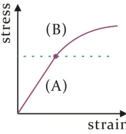
Fig. 3-1 A typical stress-strain curve... 28

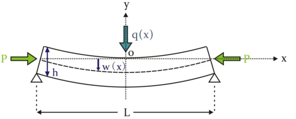
Fig. 3-2 An elastic plate pinned at its ends and bending under a load q(x) ... 31

Fig. 3-3 A segment of the deflecting plate in Fig. 3-2 ... 32

Fig. 3-4 The small segment (with the length of l) of the plate ... 35

Fig. 3-5 The phase diagram of water ... 39

Fig. 3-6 Iapetus thermal radiation image ... 40

Fig. 3-7 Illustration of vertical forces on a deflected elastic plate ... 42

Fig. 3-8 Flow chart of the analytical flexural modeling ... 45

Fig. 3-9 Flow chart of the numerical flexural modeling ... 48

Fig. 4-1 The site of DTM profiles ... 50

Fig. 4-2 Analytical Flexural Modeling of Profile r1 ... 52

(11)

viii

Fig. 4-11 Numerical Flexural Modeling of Profile r1... 58

Fig. 4-12 Numerical Flexural Modeling of Profile r2 ... 58

Fig. 4-20 Modeling of Profile r9 with Various Lithospheric Elastic Thickness. ... 61

(12)

ix

List of Tables

Table 1 Basic Parameters of Iapetus... 8 Table 2 Origin Models of Iapetus’ Equatorial Ridge ... 22 Table 3 Parameters of The Equatorial Ridge for Every Profile ... 51

(13)

1

Chapter 1 Introduction

1.1 Saturn

Saturn is the second largest planet in the Solar System. It is located on an average distance of 9.58 AU away from the Sun. This giant planet belongs to a member of Jovian Planets, and is composed of mainly gaseous matter (96.3%

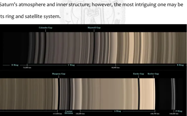
hydrogen and 3.25% helium) and a small amount of solid matter (ice and silicate rocks) as its inner core (Willians, 2012). The high ratio of gaseous matter lowers the average density of Saturn with only 687 kg/m³, which is much less than Jupiter, Uranus and Neptune (Willians, 2012). There are many interesting properties of Saturn’s atmosphere and inner structure; however, the most intriguing one may be its ring and satellite system.

Fig. 1-1 Ring System of Saturn. PIA08389, Courtesy of NASA. Horizontal

axis stands for the distance away from the center of Saturn.

(14)

2 1.1.1 The Ring System of Saturn

Saturn’s rings which consist of dust particles are multi-layered. The whole ring system can be divided into several layers by the ring gaps, whose particles are sparser than ring layers (e.g. Huygens Gap in Fig. 1-1). The particles stuffed in the rings are sized from 1 centimeter to ten meters, and constructed a vertically thin layer (Zebker et al., 1985). According to IAU nomenclature, D ring occupies the most inner part of the ring system, and the next is C, B, A, F ring and so on. Fig. 1-1 displays the relative position of the ring system. There are also some ring layers beyond the F ring; for instance, Phoebe Ring spans from ~4 million kilometers to over 13 million kilometers away from the center of Saturn (Verbiscer et al., 2009). Due to the improvement of observation technology, new rings outside the F ring are

continuously discovered. The outer edge of Saturn’s rings still remains ambiguous

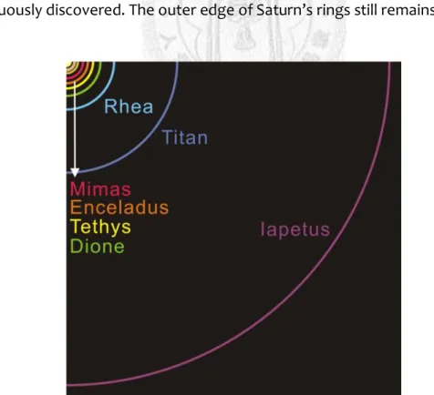
Fig. 1-2 Relative position of the major moons of Saturn.

(15)

3

since the reflected light of ring edge is too dim to detect.

The origin of Saturn’s rings is also ambiguous. Previous studies suggested that the age of the rings may be old, but the precise age remains unknown (Kerr, 2008).

The rings were interpreted to the wrecks of a satellite. After a huge impact event, the satellite was scattered into particles. For those particles which were in the Roche limit of Saturn, they remained scattered due to the affection of tidal force.

Rings may interact with nearby satellites. These satellites, often called

“shepherd moons”, help the rings to stabilize the ring system. For example, two moons Prometheus and Pandora maintain the shape of the F ring and prevent any gravitational interruption.

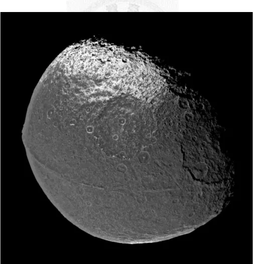
Fig. 1-3 Image of Iapetus. PIA06166, courtesy of NASA.

(16)

4 1.1.2 The Satellite System of Saturn

Saturn has numerous satellites with a high variety of features. Most of them are too small to form spheroids. Only 7 moons are ball-shaped: (arranged with the distance from Saturn) Mimas, Enceladus, Tethys, Dione, Rhea, Titan and Iapetus. Fig.

1-2 also shows the distance between each major satellites and Saturn.

The 7 moons have their own geologic features. Mimas is the smallest known gravitational rounded astronomical body in the Solar System. It’s highly

tidal-stretched, so it appears egg-shaped. Enceladus is geologically active due to cryovolcanism. Water may exist under its surface ice layer. Tethys has a large crater Odysseus and a large canyon Ithaca Chasma. These 2 features may have relationship in the early age of Tethys. Some ice cliffs exist on the surface of Dione; this perhaps implies the geologic activity similar to Enceladus. Recent researches suggested that Rhea may have its own ring system (Jones et al., 2008; Schenk et al., 2011). It would become the first satellite which has a ring around itself. Titan is the largest moon of Saturn; it is also the only satellite covered with thick atmosphere. Therefore, Titan is regard as a hotspot of astrobiology which may help us to understand the early stage of life. Finally, Iapetus is the topic of this study. The next section will discuss more details of Iapetus.

1.2 Iapetus

Iapetus is the third largest satellite of Saturn, also the 11th largest satellite in the Solar System (Yeomans, 2012). Fig. 1-3 taken by Cassini-ISS (Imaging Science

Subsystem) shows the outline of this satellite. Although its mean radius is only 734.3

(17)

5

km (Thomas, 2010), peculiar geomorphological features make Iapetus become a focus of planetary science. This section will simply introduce the basic knowledge of Iapetus, including observations and important features.

1.2.1 Observational History

Iapetus was first discovered by Giovanni Domenico Cassini in October 25^th, 1671.

After several decades of observation, he found that if Iapetus appears on the western side of Saturn, it is always brighter than viewing it on the eastern side of Saturn (van Helden, 1984). Hence, Cassini surmised that Iapetus must be tidally locked by Saturn, and that it has a brightness difference between the two sides of Iapetus. In the other words, the bright side faces the Earth when Iapetus is on the western side, and the dark side emerges when Iapetus is on the eastern side. His conjecture was confirmed by Cassini-Huygens spacecraft 2 centuries later. The dark side of Iapetus nowadays is named Cassini Regio in honor of his excellent

contribution.

After Cassini’s observation, humans didn’t know much more about Iapetus until the arrival of Cassini-Huygens spacecraft in 2007. Cassini-Huygens is a spacecraft mission conducted by NASA (National Aeronautics and Space Administration), ESA (European Space Agency) and ASI (Italian Space Agency) (Munsell, 2012). Its main goal is to study the science of Saturn and its natural satellites. Cassini-Huygens includes a Saturn orbiter called Cassini and an atmospheric probe, called Huygens, for its moon Titan. It launched on October 15^th, 1997 and reached Saturn on July 2004. Huygens probe separated from Cassini orbiter five months later, and

successfully entered Titan’s atmosphere on January 14^th, 2005. Huygens performed

(18)

6

excellently since it finally landed on Titan’s surface and returned data to the Earth.

It’s also a first probe that landed on the outer Solar System. On the other hand, Cassini orbiter investigated many aspects of Saturn during different flybys. On September 10^th, 2007, Cassini had its first and only flyby of Saturn’s distant moon, Iapetus, just 1640 km above its surface (Munsell, 2012). Many images and data were taken (Fig. 1-3), including instrumental observations of Cassini’s Visible and Infrared Mapping Spectrometer (VIMS), ISS, Composite Infrared Spectrometer (CIRS), Ultraviolet Imaging Spectrograph (UVIS) and RADAR detection (Jet Propulsion Laboratory, 2007). The observational details will be discussed in the next chapter.

After this flyby, no other flyby events or plans are suggested until 2012.

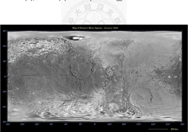
Fig. 1-4 Global Surface Image of Iapetus. PIA08406. Courtesy of NASA.

(19)

7 1.2.2 Basic Physical Properties

Most detailed physical properties of Iapetus were measured by Cassini spacecraft. Compare to the other satellites of Saturn, Iapetus has some abnormal parameters. First, from Fig. 1-2, Iapetus has the largest orbital semi-major axis and inclination among all major satellites of Saturn (Castillo-Rogez et al., 2007).

Although there are dozens of small satellites like Phoebe outside Iapetus, they are too small to form spheroids. Iapetus is big enough to maintain its spheroidal shape, but it is highly flattened. The lengths of Iapetus’ 3 axial radii are listed in Table 1.

C-axis is set to the polar radius, which is only 95% of the equatorial radius. Iapetus’

mean density listed in Table 1 is only 1.088 g/cm³. It’s also the smallest mean density in all Saturn’s major satellites. That implies Iapetus may be mainly composed of water ice (near 0.9 g/cm³) or have a porous inner structure, and silicate materials may occupy 20% or less of Iapetus’ total weight (Castillo-Rogez et al., 2007).

Another unique property of Iapetus is its albedo variability. The global topographic map of Iapetus (Fig. 1-4) was made from mosaic images taken by

Cassini ISS. Iapetus is highly synchronized with Saturn, and the terrain of the leading side (left side in Fig. 1-4, often called Cassini Regio) shows darker than Iapetus’

trailing side. The albedo is 0.05 for the leading side and is 0.5 for the trailing side (Willians, 2012). The boundary of albedo dichotomy is also obvious. This

phenomenon is exclusive in the Solar System, and becomes a highlight of Solar System science. The hypotheses of the formation of albedo dichotomy will be mentioned in the next chapter.

(20)

8

Table 1 Basic Parameters of Iapetus

Orbital Properties

Semi-major Axis (m) 3.561×10^9*

Eccentricity 0.0283^*

Inclination (°) 14.72^*

Orbital Period (days) 79.33^* Physical Properties

Mean Radius (km) 734.3±2.8^†

Oblate Semi-major Axis (km) 745.7, 745.7, 712.1^† Mean Density (kg/m³) 1088±13^†

Rotation Period (days) 79.32^‡ Equatorial Surface Gravity (m/s²) 0.220-0.223^‡

Albedo 0.05-0.5^*

Mass (kg) 1.806×10^21§

*: Willians, 2012.

†: Thomas, 2010.

‡: Roatsch et al., 2009.

§: Jacobson et al., 2006.

(21)

9 1.2.3 Surface Features

The surface of Iapetus is highly cratered. Several huge craters can be seen on Fig. 1-4. The diameter of the largest crater is 580 km, equal to ~78% of Iapetus’ mean radius (USGS Astrogeology, 2009). The fact of cratering implies 2 points at least: 1) Iapetus presently has no significant geologic processes; and 2) All the surface features on Iapetus must be old except some mass wasting events, which will be discussed in the next chapter.

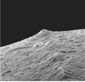
Iapetus also has the most peculiar surface feature that was uncovered by Cassini orbiter. Denk et al. (2000) have first detected it in Voyager data, but no further description until 2007 Cassini flyby. Just as previous mentioned, Iapetus has an equatorial bulge that outlines an oblate spheroid of Iapetus; but stranger than the bulge is its equatorial ridge. Equatorial ridge is a huge structure on Iapetus, and can be seen on the global view of this satellite (Fig. 1-2 and 1-4). The closer view of

Fig. 1-5 Equatorial Ridge on Iapetus. PIA08404. Courtesy of NASA.

(22)

10

the equatorial ridge is showed by Fig. 1-5 taken by Cassini orbiter. This mountain lies precisely on the equator and runs over 75% of the circumference (Singer &

McKinnon, 2011). Cassini observations (Porco et al., 2005) reported that the

equatorial ridge typically has a triangular cross-section with a base of 200 km and a height of up to 20 km. Some parts of equatorial ridge have devastated by cratering, but the well-preserved section of the ridge spans over 1600 km, that is, over one third of the circumference. The existence of the ridge do not relate to the albedo dichotomy since the ridge is continuous on the dichotomy boundary. The flanks of the ridge are steep with over 20 degrees in some areas (e.g., Giese, Denk et al., 2008). The estimated volume of this mountain is ~3×10⁶ km³ (~0.1% of total volume of Iapetus), excluding any mountain roots. The ridge is also an old structure since the surface of the ridge is dominated by craters, like other areas on Iapetus. This mountain is also the main topic of this study.

1.3 Research Goals

After the exploration of Cassini spacecraft, we could get more information about these 2 unique features (the albedo dichotomy and the equatorial ridge).

There is one intriguing question among all the research topics related to Iapetus:

how did the equatorial ridge form? Is there any distinctive process on the formation of the ridge? Until 2012, many studies on Iapetus tried to suggest models explaining the formation of the equatorial ridge. These models include despinning

(Castillo-Rogez et al., 2007), collapse of Iapetus’ ring system (Ip, 2006), contraction theory (Sandwell & Schubert, 2010), convection theory (Czechowski &

Leliwa-Kopystyński, 2008), magmatic intrusion (Melosh & Nimmo, 2009), large

(23)

11

impact event (Dombard et al., 2012). It is still under debate about which model is more possible. Therefore, this study will change the sight toward the ridge to another aspect. We first examine the possible restricted physical conditions the ridge, and the last select the more possible model for interpreting the formation of the ridge.

Flexure model is a powerful tool for analyzing the layered structure of the lithosphere on the Earth. In order to construct the inner structure of Iapetus (especially in the ridge area), this study utilizes the flexure model as a major tool.

Although there is no gravitational anomaly and laser altimeter data, Giese, Denk et al. (2008) have transferred the Cassini ISS images into the Digital Terrain Model

(DTM). They overlapped different images, which photographed the same area in Iapetus. Based on the program calculation, they gathered the more detailed DTM data of Cassini Regio on Iapetus. Most previous studies pointed out that there isn’t any flexure signal caused by the loading of the equatorial ridge (Dombard et al., 2012; Giese, Denk et al., 2008), but in this study shows the high possibility of a

thin-shell flexure signal in the foothills of the ridge. This study attempts to construct both analytical and numerical models of flexure model, and deducts the possible boundary conditions of the ridge. These conditions may correlate with some origin models. Finally, these conditions would reveal a likelihood of the ridge formation.

(24)

12

Chapter 2 Historical Researches

2.1 Geological Background of Iapetus

So far, most data and images of Iapetus are observed by the 2007 flyby of Cassini orbiter. Several models have been mentioned to construct the geologic inferences of Iapetus. These models are usually classified into different topics:

shape and rotation, inner structure, age, albedo dichotomy of exosphere, and equatorial ridge. All topics will be described next except the origin models of the equatorial ridge, which will be discussed in section 2.3.

2.1.1 Shape and Rotation

Iapetus is a satellite that has a shape of oblate spheroid (746×746×712 km, from Table 1), and its rotation period is tidally synchronized with a 79-day orbiting period (Porco et al., 2005). The highly flattened shape of Iapetus is possibly caused by rotational flattening since the amount of a-c axis difference is large enough to ignore the effect of crater modifying. But 79-day rotation period is too slow to form an oblate spheroid. Consider an equilibrium of gravitational field and centrifugal acceleration due to rotation, the flattening coefficient, f, is given by

𝑓 =

^𝑅^𝑒^−𝑅^𝑝

𝑅

=

⁵

4 𝜔²𝑅³

𝐺𝑀 (2-1)

where R is the mean radius of the satellite, Re and Rp stand for the equatorial and polar radius (a and c axis) of the satellite, ω and M are the angular velocity and the

(25)

13

mass of the satellite, and G is the gravitational constant. The parameters listed in Table 1 are adopted to calculate the status of hydrostatic equilibrium for the current rotation period. If Iapetus is homogeneous, the estimated a-c difference (Re – Rp) is only 2.53 m. It doesn’t match with the current shape of Iapetus. Thus, Iapetus doesn’t have an equilibrated shape nowadays, and must possess a despinning history.

In the meantime, the hydrostatic equilibrium of the shape of Iapetus yields a predicted period of 16.5 h (from Eq. 2-1). If there was a silicate core inside Iapetus, it would be required a spin period of 15.2 h to form this oblate spheroid

(Castillo-Rogez et al., 2007). So, Iapetus has a fossil shape that formed in the early age of Iapetus. When the rock strength of Iapetus increased due to cooling, Iapetus fixed its outline.

Another issue is that how long did Iapetus despin to the synchronization? In fact, all satellites of Saturn, except Hyperion, are tidally locked by Saturn. However,

synchronous spin on Iapetus is less possible than the other Saturnian satellites since Iapetus has both large mass and semi-major axis (Peale, 1986). Ip (2006) and

Matson et al. (2009) also suggested that Iapetus need much time that possibly more than the age of the Solar System, except that the interior are mostly molten. To describe more precisely, we uses the following formula to calculate the damping time of tidal locking (Gladman et al., 1996; Peale, 1977):

𝑡

_{𝑙𝑜𝑐𝑘}

≈

_3𝐺𝑀^𝜔^𝑖^𝑎⁶^𝐼𝑄

𝑝2𝑘₂𝑅⁵ (2-2)

where ωi is the initial angular velocity of the satellite (1.06×10^-4 radian/sec) , a is the

(26)

14

semi-major axis of the satellite, I is the moment of inertia (≈ 0.4M𝑅²) of the satellite, Q is the dissipation function of the satellite, Mp is the mass of the planet (which is Saturn in this case, 5.6846×10²⁶ kg (Willians, 2012)), k2 is the tidal Love number of the satellite. In general,

𝑘

₂

≈

^1.5

1+_{2𝜌𝑔𝑅}^19𝜇 (2-3)

where μ is the rigidity of the satellite (usually 4×10⁹ Nm^-2 for icy satellites), ρ is the mean density of the satellite, g is the surface gravity of the satellite. Set a generic Q of solid bodies = 100, Eq. 2-2 and 2-3 yield a tidal-locking time of 277 My. Since Q has a high uncertainty which ranged from 10-500 for solid icy satellites (Dobrovolskis et al., 1997), Iapetus may have a tidal dissipation timescale of 28-1400 My. Based on the

calculation, we can conclude that it requires the existence of partial melting on the early stage of Iapetus inner core to synchronize its spin, or Iapetus may have spent long time (roughly 100-1000 My) to do so.

2.1.2 Age

Porco et al. (2005) reported that Cassini ISS images showed the heavily cratered surface of Cassini Regio. The whole surface except the equatorial ridge area is controlled by the cratering, with over 3 large ones whose diameters are larger than 350 km. The study of size distribution of craters (Kirchoff & Schenk, 2010) suggests that the terrain age of both dark side and bright side are the same. The high density of craters on Iapetus implies that Iapetus may be geologically old.

(27)

15

A quantitative value of the age of Iapetus is predicted by Castillo-Rogez et al.

(2009, 2007). They set a model considering the shape, despinning and the thermal history of Iapetus, and the best-fit age value is between ~3.4-5.4 Myr after the formation of calcium-aluminum inclusions (CAIs). The age of CAIs was measured by Amelin et al. (2002), who proposed an age of 4567.2±0.6 Myr from Pb-Pb dating method. Thus the age of Iapetus is 4563.8 to 4561.8 My. Since all the surface features on Iapetus appear old, they might form on the early stage of Iapetus. The crater frequencies analyzing result (Neukum et al., 2005) also implied an over 4-billion-year surface on Iapetus. Based on lunar crater studies, the age of the surface of Iapetus is probably close to 4400-4500 Myr.

2.1.3 Inner Structure and Composition

As previous mentioned, Iapetus has 2 possible internal structures: 1) Iapetus has large portion of low-density materials; 2) Iapetus has a porous inner core. If Iapetus is composed of low-density materials, then water ice is the most likely matters since ice has a low density (0.9 g/cm³) similar to the density of Iapetus. In the model proposed by Leliwa-Kopystyhski et al. (1994), Iapetus is set to have an icy mantle of 418-km thickness and an silicate inner core (whose density is 3.361 g/cm³) of 328-km radius. But the radius of the inner core decreases when mantle is mixed with

ammonia (NH3) and methane (CH4), which are the bulk compounds in the Jovian planets. In the other hand, Owen et al. (2001) analyzed the infrared spectrum of 0.3-3.8 μm to get the information of the surface composition of Iapetus. They found that the surface of Cassini Regio is deposited by the mixed matters of water ice, amorphous carbon, and nitrogen-rich compounds. After Cassini orbiter’s

(28)

16

observation, Buratti et al. (2005) obtained the VIMS data for Iapetus, and concluded that the bright side is ice-rich so that it appears the high albedo; and that the

detection of carbon dioxide (CO2) in the dark side implies the removal of the regolith. Cruikshank et al. (2010) even noted that the CO2 on Iapetus is native, enclathrated in water ice, and then released due to the exposure of the solar wind.

Therefore, an acceptable model is that the bulk composition of Iapetus is H2O, and that there are compounds which are rich in carbon, nitrogen inside the water ice.

A porous inner core may exist, but is less possible due to a lack of gravitational data. Sandwell and Schubert (2010) used this hypothesis to construct a model of the formation of the equatorial ridge, which will be discussed later.

2.1.4 Thermal History

Thermal history is the key to the chronology of Iapetus. If the tidal-dissipating time is relatively short, sufficient heat is needed for the partial melting of the inner core. Furthermore, the fossil 16-h shape implies a core which generated large amount of heat but lost it quickly. Castillo-Rogez et al. (2007) noted that ²⁶Al could play a significant role on the early stage of Iapetus. ²⁶Al is one of short-lived

radioactive isotopes (SLRI), which include the common radioactive isotopes with the half-life of under several million years. ²⁶Al is also abundant in CAIs, but quickly decay to ²⁶Mg with a half-life of 0.716-0.73 Myr (Kita et al., 2005). Castillo-Rogez et al.

(2009) also pointed out that the abundance of ²⁶Al dominated the age, the porosity changes, and the shape evolution. Their modeling result shows a possible ²⁶Al-rich scene: after Iapetus formed (with the age mentioned in section 2.1.2), the heating from radioactive nuclides lowered the strength of the material of Iapetus, shaped

(29)

17

an oblate spheroid. When Iapetus synchronized its spin within 200-1000 Myr, no more ²⁶Al radioactive heat was generated so that the satellite was cooling down, remaining a 16-h fossil shape.

2.1.5 Albedo Dichotomy

Iapetus’ albedo dichotomy can be easily recognized in Fig. 1.4. The Cassini Regio (dark side) distributes over low to mid-latitude regions, and is constrained in 0-210 degrees of longitude. Squyres and Sagan (1983) first noted that there is a

one-magnitude difference of albedo between the dark side and the bright side. The VIMS survey mentioned in 2.1.3 offered a possible composition of these 2 sides (Buratti et al., 2005; Cruikshank et al., 2010): The bulk composition of the bright side is water ice, however the matters on the dark side mixed with several compounds including H2O, CO2, and N-rich organic compounds which are often called tholins.

Because we observed that CO2 emited from ice clathrates, it is accepted that the dark side is regolith-depleted; in other words, the deep rock of Iapetus is exposed to the surface because of the removal of the weathering soil.

Dozens of hypotheses were proposed to explain the origin of the dichotomy.

For instances, Owen et al. (2001) interpreted the dark side as debris deposits, which were originated from Titan. On the other hand, Marchi et al. (2002) regarded the dichotomy as a result of Iapetus-Hyperion collision event. Wilson and Sagan (1996) also suggested that there is a removal of ice on the dark side, and then the dark matters were exposed; the trigger of the removal of ice is numerous impact events from interplanetary dust particles. Most of these hypotheses are related to

exogenic procedures. In the recent study, a new model is illustrated by Spencer and

(30)

18

Denk (2010), who plausibly explained the albedo dichotomy as a global thermal migration of water ice. In this model, a slight albedo difference is given in the beginning. Since Iapetus has an unusual synchronous spin, the day temperature is high enough to sublimate water ice. If there is a slight albedo dichotomy on Iapetus, water ice in the dark side will be sublimated during daytime. The gaseous H2O will migrate and deposit in the bright side, and then increase the albedo of the bright side. This positive feedback enlarges the difference of the two sides, and finally depletes the water ice in the dark side. The process costs 2400 Myr to form the nowadays condition of Iapetus. Because Iapetus need ~10⁹ years to be synchronized, the albedo dichotomy may be a “new” structure on the Iapetus, or still in

development.

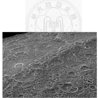
Fig. 2-1 Portion of image N1483174398. From Porco et al. (2005).

(31)

19

2.2 Geomorphological Data of Iapetus’ Equatorial Ridge

The earliest mosaic images of Iapetus are published by Porco et al. (2005). Fig.

2-1 is one of the images of the peculiar equatorial ridge. The ridge in Fig. 2-1 shows 2 features: 1) several parallel linear structures aligning the ridge; and 2) heavily

cratered surface with some parts which is devastated (the lower left corner of the ridge in Fig. 2-1).

To obtain more detailed morphological data of Iapetus, Thomas et al. (2007) employed the limb coordinates and stereogrammetric control points which were measured by the Cassini ISS. They treated Iapetus as an oblate spheroid with

747.4×747.4×712.4 km. And the next, the limb area (especially in the equatorial bulge) of each image is located and measured. Finally, Thomas et al. gathered 31 limb

profiles of the equatorial bulge area. However, Giese, Denk et al. (2008) pointed out that the limb profile may be over-estimating on the height of the equatorial ridge.

They used another way to construct the Digital Terrain Model (DTM) data of Iapetus.

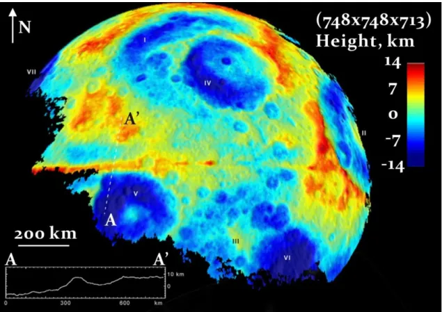
Their simple idea is to superimpose multiple images which have control points and picture at the same area of Iapetus. The shadowed area that is caused by the highlands of Iapetus varies when the position of the orbiter changes, so the height of the surface is obtained by superimposing images taken by Cassini ISS from different places. Giese, Denk et al. utilized their method to icy satellites including Enceladus (Giese, Wagner et al., 2008), Phoebe (Giese et al., 2006), and of course Iapetus. Fig. 2-2 displays the calculated DTM data of leading side (dark side). (Giese, Denk et al. also noted that the DTM height of the ridge is 10-20 km, which a width of 100-200 km and an average slope of 4-10 degrees. The DTM data shows a lower

(32)

20

ridge than previous suggestion by Thomas et al. (2007), but the precision of the surface profile is enhanced. For example, the A-A’ profile in Fig. 2-2 cuts through a crater, the ridge, a depression area and a plateau area; this profile distinguishes them respectively. The resolution of DTM data is kilometer-scale, but the small structure of such this scale may be ignored when modeling; that is, DTM data is useful on large-scale structures like big craters or the ridge, but it is not so precise for the small structures.

Fig. 2-2 Digital Terrain Model (DTM) of Iapetus. Reference shape is a 748×748×713

oblate spheroid. A-A’ profile cuts though the depression area, the ridge and crater No. 5. Modified from Giese, Denk et al. (2008).

(33)

21

2.3 The Origin Models and Flexural Implications of Iapetus’ Equatorial Ridge

The equatorial ridge is also an old structure since the crater density is similar to the other areas of Iapetus. If we accept the crater-frequency dating proposed by Neukum et al. (2005), the ridge has remained its shape for over 4 billion years.

Although there is a fossil 16-h equatorial bulge, the ridge seems to be excluded from the bulge and superimposes on it. Obviously, the ridge was not formed simply by despinning, and the other scene is needed to explain the origin of the ridge.

Until 2012, the ridge has been interpreted into several different origins, which can be divided into two main classes: endogenic model and exogenic model. Due to the lack of in situ survey, it is still under debate that which one is more correct. The brief descriptions of these models are listed in Table 2 for the detailed discussion in the next section.

(34)

22

Table 2 Origin Models of Iapetus’ Equatorial Ridge

Author(s) and year Model Class Description

Ip (2006) Exogenic The collapse of the ring system, which originated during Iapetus’ formation Castillo-Rogez et al.

(2007); Porco et al.

(2005)

Enodogenic Tectonic activity triggered by the despinning

Dombard et al. (2012);

Levison et al. (2011)

Exogenic The collapse of the ring system, which originated from an impact event Giese, Denk, et al.

(2008)

Endogenic Endogenic tectonic unwarping (fold)

Czechowski and Leliwa-Kopystyński (2008)

Endogenic The rising point in the two-cell convection

Melosh and Nimmo (2009)

Endogenic Igneous dike intruded in a thin lithosphere

Sandwell and Schubert (2010)

Endogenic Lithosphere was applied by the contraction stress, which originated from a porous core

(35)

23 2.3.1 Exogenic Models

Porco et al. (2005) first noted that the equatorial ridge may originate from the same process that formed the equatorial bulge. Castillo-Rogez et al. (2007)

expanded this idea and developed a model to evaluate the possibility of a despinning scenario. In this model, the ridge is interpreted to what was buckled when Iapetus started to slow down its rotation from a high initial spin rate. Set the thickness of lithosphere is 15 km, and then a 5-h initial spin rate is adequate to redistribute enough amount of material (~3.5×10⁶ km³) that reaches the volume of the ridge (~3×10⁶ km³). Although there’s a high uncertainty affected by the

lithospheric thickness, the initial spin rate is so close to the 3.8-h Roche limit that it hardly maintain a shape of oblate spheroid.

Therefore, the dispinning scenario is doubtful. Ip (2006) computed that the despinning has not likely finished for limited age of the Solar System, just as discussed in section 2.1.1. He also suggested a new exogenic model that describes the ridge as deposits of a ring system remnant. Just like Saturn or the other gaseous planets, satellites may have their ring system during the formation stage. Iapetus’

dust particles in the ring system might collide and drag with each other, making a dissipation of energy. This condition resulted in the decay of the ring orbit, and that numerous particles impacted on the equator of Iapetus, accumulating an equatorial ridge. Similar phenomenon was recently discovered on another Saturian satellite, Rhea, which has a completed equatorial linear trace that was soon interpreted as a ring remnant, although the total mass is much lesser than the equatorial ridge (Schenk et al., 2011). Ip also proved that the possible volume of the Iapetus ring is sufficient to accrete the nowadays equatorial ridge. Fig. 2-3 simply describes the

(36)

24

process he proposed, and it makes sence that why the ridge lies precisely on the equator.

Based on the previous idea, the exogenic model has been developed by Levison et al. (2011) and Dombard et al. (2012). These two studies suggested that an ancient

giant impact created Iapetus’ ring system. Dombard et al. noted that if both Iapetus and its ring system have formed from the Saturian subnebula, it would have not been explained why the equatorial ridge was only found in Iapetus. Alternatively, they proposed the model that the ring formation may be posterior to the formation of Iapetus due to a unique catastrophic incident on Iapetus. Levison et al. (2011)

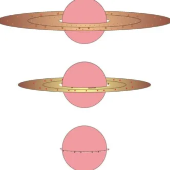
Fig. 2-3 Illustration for a ring-collapsing scenario, modified from Ip (2006). Top:

Iapetus owned its ring system. Middle: The ring system gradually decayed its orbital radius due to the tidal dissipation. Bottom: The remnant of the ring deposited on the equator of Iapetus, building the ridge. Dombard et al. (2012) and Levison et al. (2011) used similar process to explain the transformation from an impact event to the equatorial ridge.

(37)

25

presented a scenario that the impact debris built the ring straightly; while Dombard et al. (2012) proposed that the impact may form a subsatellite first, and then this

subsatellite decayed its orbit, eventually entering the Roche limit of Iapetus, torn into pieces, building the ring indirectly. After the ring formed, the accumulation scene is similar to Fig. 2-3.

2.3.2 Endogenic Models

Some researchers preferred endogenic models which need some special structural conditions. Giese, Denk et al. (2008) first pointed out that the ring remnant deposits should build a steep hill and a sharp peak, whose angle of

response is up to 30-40 degrees. However, the average slope of the equatorial ridge is only 8-15 degrees (Giese, Denk et al., 2008), and the topography of the peak revealed by their DTM model is really flat. Therefore, they argued that the ridge may not be formed by an exogenic process, but an ancient tectonic activity. Steep slopes and top-flatted peaks can be simply attributed to tectonic upwarping. They also figured out that there are some depressions aligned with the equatorial ridge; these depressions may stand for the flexural signals.

Next, Sandwell and Schubert (2010) expanded their study for the equatorial ridge. They suggested an innovative model describing a porous inner core (where porosity is over 10%) and a solid outer shell in Iapetus’ early stage. When the inner core was heated and reached about 200K, the core began shrinking and lost the support force to the outer shell. Then the shell must deform its shape to match the volume with the inner core. The equatorial ridge is such a product of this buckling process. If the ridge was buckled, the flexure model can be used to construct a

(38)

26

relation between the thickness of the outer shell and the buckling type. This model in the spheroid case is suggested by the following formula (Beuthe, 2008; Sandwell

& Schubert, 2010):

𝑊_𝑙 = 𝑞₀[^𝜂𝐷

𝑅⁴

𝑙(𝑙+1)[𝑙(𝑙+1)−2][𝑙(𝑙+1)−2]

[𝑙(𝑙+1)−1+𝜐] − ^𝐹

𝑅²

[𝑙(𝑙+1)−2][𝑙(𝑙+1)−2]

[𝑙(𝑙+1)−1+𝜐] +

𝐸ℎ 𝑅²

[𝑙(𝑙+1)−2]

[𝑙(𝑙+1)−1+𝜐]+ Δ𝜌𝑔]⁻¹ (2-4)

𝜂 =

^12𝑅²

12𝑅²+ℎ² (2-5)

where W is the vertical deformation (flexure value) in terms or Legendre

polynomials, q0 is the vertical load, D is flexural rigidity which will be mentioned in Chapter 3, R is the radius of the satellite, E and ν are Young’s modulus and Poisson ratio of the material, F is the end load, h is the thickness of the lithospheric outer shell, Δρ is the change of density between the core and the space (where the value is equal to ρ), and g is the surface gravity of the satellite. The l value in Eq. 2-4 is a factor of the frequency domain, and l=2πkR approximately. The denominator of Eq.

2-4 explains a composition of flexural frequencies. The lesser the amount of the denominator is, the larger the portion of the flexure is. Sandwell & Schubert found that if the buckling forms the type of the ridge whose harmonic degree (=2πR/λ =kR) is 2, the thickness of the lithospheric shell should excess 120 km. This model is

plausible since it does not need an ultra-high initial spin rate of 5-h and a strictly constrained thermal history. Nevertheless, it can’t explain the depressions aligned with the ridge because thick shell didn’t cause obvious regional depressions.

(39)

27

Another different endogenic model was proposed by Czechowski and

Leliwa-Kopystyński (2008). Their model assumed a convective flow inside Iapetus.

The properties of the material and the amount of the heat flow both affect the convective patterns. If parameters are chosen properly, Iapetus will show a pattern of 2-cell convection. In the 2-cell convection, the heat material flow upwells in the equator, and subducts in the polar region. In other words, the role of the ridge is like the mid-ocean ridges on the Earth. The disadvantages of this model is that we don’t find any structures implying subduction near the pole of Iapetus; moreover, it’s difficult to build such a high ridge only pushed by the thermal buoyancy (Dombard & Cheng, 2008).

Besides, there is also a creative model suggested by Melosh and Nimmo (2009).

They regarded the ridge as an intrusive dike which occurred where the shell is the thinnest and hottest. It’s similar to the scene of convection model, but they noted that the model doesn’t need any convective patterns. When tidal dissipation generated heat on Iapetus, the heat soon concentrated in the Iapetus’ equator, thinning the lithosphere. Thus, heat flow upwelled in the equator, generated a ridge.

(40)

28

Chapter 3 Research Methods

3.1 Introduction to the Flexure Model

Flexural model originates from the studies of lithosphere and plate tectonics on the Earth. This theory was first developed in the 1970s for the rising of the theory of plate tectonics. 3 main geomorphological observations imply the lithosphere may obey the elastic deformation mechanism: 1) post-glacial rebound; 2) the gravity anomaly of the seamount chains; 3) the buckling of the convergent plate boundary.

Walcott (1970) proposed a concept that the upper lithosphere must deform elastically because the temperature and the pressure are low here. Although Walcott noted that the proper description of the lithospheric deformation is viscoelasticity in large time scale, the model only considering elasticity is worth to be a reference model since it is simple and has minor bias.

Material behavior is mostly constrained by stress, temperature and pressure.

Fig. 3-1 shows the typical stress-strain curve of the material, and this curve is divided

Fig. 3-1 A typical stress-strain curve.

(41)

29

into (A) and (B) regions. In (A) region, stress is proportional to the strain, and the material obeys elastic deformation (Hook’s law); In (B) region, stress is beyond the elastic limit (the boundary stress of (A) and (B) region), the material deforms plastically or is fractured (brittle deformation). The elastic limit which controls the type of deformation is affected by both temperature and pressure. If temperature and pressure are low, material shows mainly elasticity.

In the theory of plate tectonics, the plate must be applied an end load (by the tectonic force) and a vertical load (by the surface deposits). If we ignore the brittle deformations such as faults and fractures, the whole plate can be treated as an elastic material. Thus, the geomorphological features and the gravity anomaly are the outcome of the bending plate, and then the thickness of this plate can be found out by solving formulae listed in the next section. This thickness is also called the

“elastic thickness of lithosphere”. Studies showed that the elastic thickness of oceanic lithosphere is ranged from 2-50 km, and that the elastic thickness of continental lithosphere is scattered with 5-100 km (Watts et al., 1982). The elastic thickness cannot represent the thickness of whole lithosphere since the lower lithosphere may deform plastically, but it is highly bound with geothermal gradient or thermal conductivity. For example, the elastic thickness increases when the age of sea-floor increases because the older sea-floor has the smaller geothermal gradient, enlarging the thickness affected by elastic deformation (Watts et al., 1982).

3.2 Construction of the Flexure Model

The flexure model is built on the elastic plate theory, which has been well

(42)

30

studied for mechanical engineers for several tens of years. The structure of the flexure model in this paper mainly refers to the books, separately written by Watts (2001) and Turcotte and Schubert (2002). It will be simply described.

3.2.1 Fundamental Formulae of the Flexure Model

It’s generally assumed that an elastic plate can be described by Hook’s law; that is, the stresses originating from the bent plate are proportional to the strain. Thus, we will first introduce basic relationships of the stress and strain. Consider a 3-D stressed material, and define that the scalar components of stress vectors (σ) and strain vectors (ε) exerting on the x, y, z axis are σ1, σ2, σ3, and ε1, ε2, ε3 respectively.

The relationship between stress and strain is described by the following 2

parameters: 1) Young’s modulus (E), which represents the ratio of the axial strain to the axial stress in a laterally unrestricted material; 2) Poisson’s ratio (ν), which represents the ratio of lateral extension to longitudinal extension in a laterally unrestricted material exerted by the axial stress. With these 2 parameters, the connection between stress and strain can be easily written as

𝜀

₁

=

¹

𝐸

𝜎

₁

−

^𝜈

𝐸

𝜎

₂

−

^𝜈

𝐸

𝜎

₃ (3-1)

𝜀

₂

=

^−𝜈

𝐸

𝜎

₁

+

¹

𝐸

𝜎

₂

−

^𝜈

𝐸

𝜎

₃ (3-2)

𝜀

₃

=

^−𝜈

𝐸

𝜎

₁

−

^𝜈

𝐸

𝜎

₂

+

¹

𝐸

𝜎

₃ (3-3)

Given distinctive stress and strain conditions, these stress and strain

components can be solved by Eq. 3-1 to 3-3. A common assumption used in geology

(43)

31

is uniaxial strain, that is, when sediments were buried, it would be laterally constrained. Thus, ε2=ε3=0, and Eq. 3-1 to 3-3 will be simplified to

𝜎

₂

= 𝜎

₃

=

^𝜈

1−𝜈

𝜎

₁ (3-4)

𝜎

₁

=

(1+𝜈)(1−2𝜈)^{(1−𝜈)𝐸𝜀}¹ (3-5)

In the next section, we will discuss the conditions on elastic plates, and illustrate the flexure equations from the above formulae.

3.2.2 2-D Flexure Equations of Elastic Plates

Consider an elastic plate shown in Fig. 3-2. The plate has a width (x-direction) of L and a thickness (y-direction) of h, and is infinitely long in the z-direction. A line force q(x) in unit of z direction (Nm^-2) applies on the plate and bends it. Note that q(x) will not change if z coordination varies. We define the deflection function w(x) to describe the vertical displacement of the plate. For example, a downward

Fig. 3-2 An elastic plate pinned at its ends and bending under a load q(x).

(44)

32

displacement w(x) shown in Fig. 3-2 is considered negative. The plate is pinned at its ends, that is, w is always equal to 0 on the edge of the plate. To simplify calculation, we assume that the plate is thin compare to its width, h<<L, and so is the deflection function, w<<L. Therefore, the linear elastic equations could adapt to this case. This 2-D bending case is often called cylindrical bending since the plate is a beam taken from a cylindrical shape of the bending.

Fig. 3-3 shows a segment of the deflecting plate. The deflection is the outcome of the equilibrium with all the forces and torques in Fig. 3-3. The small segment has a coordination of x and a width of dx. The downward load q(x) is exerted on the segment, so the combined downward force between x and x + dx is q(x) dx (Nm^-1).

Another force in the vertical direction is the shear force, which is V at location x and V + dV at location x + dx. Obviously, dV is also a downward force because the

segment is sheared by the adjacent segments and the right side has a stronger upward shear force. Thus, a force balance in the vertical direction can be

Fig. 3-3 A segment of the deflecting plate in Fig. 3-2, with applied forces and

torques. Modified from Turcotte and Schubert (2002).

(45)

33 constructed by equilibrating these 2 forces:

𝑞(𝑥)𝑑𝑥 + 𝑑𝑉 = 0

(3-6)

On the other hand, there are 3 types of torque acting on this segment. One is the net bending moment, which is the integrated moment on the cross section of the segment. The moment originates from the normal stresses of the cross section σxx, also known as fiber stresses. The bending moment is M at x and is M + dM at x + dx. Based on the same reason of the direction of dV, dM is considered

counterclockwise. The other torque is attributed by the horizontal force P (Nm^-1, per unit length in the z direction). The values of P in the both side of the segment are the same, but the y coordination is different. The deflection is w at x and is w + dw at x + dx, so the vertical distance of acting points of the two sides is dw. It results in a counterclockwise torque of –P dw. The minus sign is needed since dw is obviously negative, just mentioned before. The third one is the torque created by the shear force. The moment arm of the shear force is the width of this segment dx, so the torque is V dx clockwise. (The torque produced by dV can be ignored since dV and dx are both infinitesimal.) A torque balance of all the above yields

𝑑𝑀 − 𝑃𝑑𝑤 = 𝑉𝑑𝑥

(3-7)

Differentiate Eq. 3-7 twice, ant it gives

(46)

34 𝑑²𝑀

𝑑𝑥²

=

^𝑑𝑉

𝑑𝑥

+ 𝑃

^𝑑²^𝑤

𝑑𝑥² (3-8)

Substituting Eq. 3-6 into Eq. 3-8 obtains

𝑑²𝑀

𝑑𝑥²

= −𝑞 + 𝑃

^𝑑_𝑑𝑥²^𝑤₂ (3-9)

The next step will be to find an expression of M in a function of deflection. M is the integration of the fiber (longitudinal) stress σxx; to find σxx, we construct a relationship between fiber stress and longitudinal strain εxx. Fig. 3-4 shows a small section of the bending plate with an infinitesimal length l. R and φ in this figure are the radius and the angle of curvature of this section respectively. The length change Δl is proportional to the distance (y component) from the midplane (y = 0). Thus, the longitudinal strain is obtained by the following equation:

𝜀

_𝑥𝑥

= −

^𝑑𝑙_𝑙

= −

^𝑦𝜙_𝑙

= −

^𝑦_𝑙 _𝑅^𝑙

= −

^𝑦_𝑅 (3-10)

(47)

35

Note that εxx is negative when y is positive; that is, compressional strain is defined negative in Eq. 3-10. The radius of local curvature is the reciprocal of the curvature κ. The expression of curvature is given by

κ =

¹

𝑅

=

⁽

𝑑2𝑤 𝑑𝑥2) [1+(^𝑑𝑤_𝑑𝑥)²]

32

≈

^𝑑²^𝑤

𝑑𝑥² (3-11)

If the slopes is small (as our assumption of w << L), the denominator of Eq. 3-11 will reduce to 1. So the curvature is equal to the second differentiation of the

Fig. 3-4 The small segment (with the length of l) of the plate. Strain

varies with y value. Modified from Turcotte and Schubert (2002).

(48)

36

deflection. Substitute Eq. 3-10 with Eq. 3-11, and then we have

𝜀

_𝑥𝑥

= −𝑦𝜅 = −𝑦

^𝑑²^𝑤

𝑑𝑥² (3-12)

In Fig. 3-2, this plate illustrates the conditions of stresses and strains. Because the plate is infinitely long in the z direction, it won’t be stretched and compressed in this direction. Hence, εzz = 0. Moreover, the stress normal to the surface, σyy, can be set to 0 throughout since the plate is thin and is on the top. Thus, Eq. 3-1 and 3-3 will be rewritten as

𝜀

_𝑥𝑥

=

_𝐸¹

(𝜎

_𝑥𝑥

− 𝜈𝜎

_𝑧𝑧

)

(3-13)

𝜀

_𝑧𝑧

=

_𝐸¹

(𝜎

_𝑧𝑧

− 𝜈𝜎

_𝑥𝑥

) = 0

(3-14)

Therefore, the fiber stress will be obtained:

𝜎

_𝑥𝑥

=

^𝐸

1−𝜈²

𝜀

_𝑥𝑥

= −

^𝐸𝑦

1−𝜈² 𝑑²𝑤

𝑑𝑥² (3-15)

The integration of fiber stresses is called the bending moment M:

𝑀 = ∫

_{−ℎ 2}^{ℎ 2}^⁄_⁄

𝜎

_𝑥𝑥

𝑦𝑑𝑦 =

^−𝐸

1−𝜈² 𝑑²𝑤

𝑑𝑥²

∫

_{−ℎ 2}^{ℎ 2}^⁄_⁄

𝑦

²

𝑑𝑦 =

^−𝐸ℎ³

12(1−𝜈²) 𝑑²𝑤

𝑑𝑥²

(3-16)

(49)

37

We define the coefficient as the flexural rigidity, D, because it is usually used:

𝐷 ≡

_12(1−𝜈^𝐸ℎ³ ₂₎ (3-17)

Thus,

𝑀 = −𝐷

^𝑑²^𝑤

𝑑𝑥² (3-18)

Substituting Eq. 3-18 into Eq. 3-9 gathers the most common formula of the deflection of the plate:

𝐷

^𝑑⁴^𝑤

𝑑𝑥⁴

= 𝑞(𝑥) − 𝑃

^𝑑²^𝑤

𝑑𝑥² (3-19)

Note that D (flexural rigidity) is the property of the material, q(x) is the summation of the vertical force, and P is the summation of the horizontal force.

Both q and P are in unit of the z direction (Nm^-1). Eq. 3-19 will be the most fundamental formula in the next discussion, which tries to apply the case of the equatorial ridge into the deflection equation.

土衛八伊阿珀托斯赤道脊之彈性折彎模型模擬

National Taiwan University Master Thesis

Elastic Flexure Model of Iapetus’ Equatorial Ridge

Acknowledgement

摘要

Abstract

Table of Contents

List of Figures

List of Tables

Chapter 1 Introduction

Chapter 2 Historical Researches

𝑓 =

=

𝑡

≈

𝑘

≈

𝜂 =

Chapter 3 Research Methods

𝜀

=

𝜎

−

𝜎

−

𝜎

𝜀

=

𝜎

+

𝜎

−

𝜎

𝜀

=

𝜎

−

𝜎

+

𝜎

𝜎

= 𝜎

=

𝜎

𝜎

=

𝑞(𝑥)𝑑𝑥 + 𝑑𝑉 = 0

𝑑𝑀 − 𝑃𝑑𝑤 = 𝑉𝑑𝑥

=

+ 𝑃

= −𝑞 + 𝑃

𝜀

= −

= −

= −

= −

κ =

=

≈

𝜀

= −𝑦𝜅 = −𝑦

𝜀

=

(𝜎

− 𝜈𝜎

)

𝜀

=

(𝜎

− 𝜈𝜎

) = 0

𝜎

=

𝜀

= −

𝑀 = ∫

𝜎

𝑦𝑑𝑦 =

∫

𝑦