國立臺灣大學公共衛生學院流行病學與預防醫學研究所 碩士論文
Graduate Institute of Epidemiology and Preventive Medicine College of Public Health
National Taiwan University Master Thesis
寇斯與隨機漫步統計模式於動態複雜型排序資料:以糞便 免疫潛血濃度為例
Cox and Random Walk Statistical Models for Dynamics of Intractable Ordinal Data: An Example of Fecal Hemoglobin Concentration
彭思敏 Szu-Min Peng
指導教授:陳秀熙 博士 Advisor:Hsiu-Hsi Chen, Ph.D.
中華民國 104 年 05 月
國立臺灣大學碩士學位論文 口試委員會審定書
論文中文題目
寇斯與隨機漫步統計模式於動態複雜型排序資料:以糞便 免疫潛血濃度為例
論文英文題目
Cox and Random Walk Statistical Models for Dynamics of Intractable Ordinal Data: An Example of Fecal Hemoglobin Concentration
本論文係 彭思敏 君(學號 R02849033)在國立臺灣大 學 流行病學與預防醫學研究所完成之碩士學位論文,於民國 104 年 05 月 29 日承下列考試委員審查通過及口試及格,特此證 明。
口試委員:
致謝
能夠完成這篇論文,我首先要特別感謝我的指導教授陳秀熙老師。謝謝陳老 師在學生的兩年碩士中給予的一切幫助與指導,不論是在課業上時常以生活中的 範例來解釋生物統計與流行病學,或是在做論文時的耐心指導以及幫助學生做修 改等等的鼓勵,感謝陳老師花費了許多的精力與時間教導學生。感謝口試委員張 淑惠老師、丘政民老師以及林明薇老師能夠在學生論文口試時撥冗參與,並給予 了許多地指正與建議,使我能夠再次以更完善的角度檢視這份論文,同時在相關 知識方面帶給我很多的收穫,最後得到了老師們一致的肯定,學生由衷的感恩。
此外還要感謝嚴明芳老師、陳立昇老師、范靜媛老師還有邱月暇老師,謝謝 老師們在學生做論文當中給予的種種指導,不厭其煩地傾聽我的問題,從統計到 程式編寫上,都一一點出學生的錯誤並且提供很多建議使我能正確地修正論文。
同時感謝 533 的所有學長、姊們,在我提出問題時總是陪伴在旁邊給予幫忙,時 常地給予鼓勵、分享經驗使得我在碩士兩年間可以快速地進入狀況。
兩年在流預所的日子裡,要感謝同樣是成大幫的小萱,不管是快樂的、忙碌 的、無趣的都一起經歷了,並且同樣期待之後也是連體嬰般的職場生活。也謝謝 生統碩二的大家,佳純、良珂一起回家不孤單,隔壁桌的芸婕常常一起討論一起 進步,碩研室的大家一起生活,做論文再忙也有你們相挺,就算偶爾疲憊也會被 激勵出更多的腎上腺素。謝謝因為進入 533 認識的古玫生,加油打氣總是來的剛 剛好。感謝管家阿祐打理我的身體健康,總是在忙碌時給予溫暖支持,但也同時 要求我投資自己的健康。最重要的還要感謝家人們,給予不匱乏的物資以及精神 鼓勵,讓我得以在這兩年內心無旁鶩的讀書做研究,感謝你們給的單純幸福。
最後,僅將此論文與各位分享,歡喜相聚,祝福滿滿。
彭思敏 謹致 于臺灣大學流行病學與預防醫學研究所
中文摘要
背景
糞便潛血濃度(f-Hb) 已證實對於大腸直腸癌的發生率以及死亡率具有極佳的 預測力。因此對於在族群篩檢而言,f-Hb 在篩檢時之重複測量數值以及其動態變 化對於族群的風險而言亦具有其重要的角色。然而,在運用族群篩檢資料發展描 述 f-Hb 變化的模型時,由於其序位型資料特性以及資料中所包含的相關性、設限 以及截切等特性,使得模型的建構極為困難。本研究利用有吸收性境界 (absorbing barrier) 之隨機漫步模型(random walk model) 將上述特性納入考量建構描述族群 f-HB 動態變化之模式。
目的
本篇論文第一個目的為利用存活分析的模式評估在不同篩檢組別(正常、大腸 腺瘤、大腸直腸癌症) f-Hb 的差異表現,並分別估計並得到族群發生大腸腺瘤以
及大腸直腸癌症的糞便潛血濃度數值中位數(f-Hb50),以及其不同的臨界值。本片
論文第二個主要的目的為應用隨機漫步模型來量化 f-Hb 濃度的動態變化,並加以 考慮在族群發生大腸腺瘤以及大腸直腸癌症時的最大上界值(即觸及吸收境界)的 情況。
方法
我們首先利用傳統的單因子變異數分析以及存活分析針對 f-Hb 在不同篩檢組 別(正常、大腸腺瘤、大腸直腸癌症)平均數或是中位數的差異進行檢定。接著運用 寇斯等比例風險模型(Cox proportional hazards regression model)控制可能的影響變 項,並且將資料中的相關特性納入考慮,以序位方式對 f-Hb 數值進行排序,估計 各組別(正常、大腸腺瘤、大腸直腸癌症)之對比風險值。配合無母數排序的方法,
吾人可以在上述三個組別中計算其糞便潛血濃度數值中位數(f-Hb50),並且分別估
計得到族群發生大腸腺瘤以及大腸直腸癌症的 f-Hb 之臨界值。
在建構動態隨機模型方面,藉由運用隨機漫步模型,並發展基於該模型的漸 進分佈(asymptotic distribution) 和多項分佈(multi-nominal distribution) 來描述 f-Hb 重複測量資料變化的進程,並估計 f-Hb 在三種不同的疾病狀態下的數值升高機率 (p) 以及降低(q)。進一步可以利用估計得到的機率估計值,計算各組別(大腸直腸 癌症或大腸線瘤病患)相對應的賭徒破產機率(即觸及吸收境界之機率)。
結果
利用經過自然對數轉換後的 f-Hb 所作的變異數分析結果中,顯示出三個組別 的糞便潛血濃度平均數值達到顯著性的差異 (F=104324, p<0.001, R2=0.142),無母 數方法檢定的結果顯示同樣顯著差異 (p<0.001)。
利用寇斯比例風險模型分析在將其他解釋變相納入調整後(性別、年齡、家族 病史以及篩檢工具廠牌),以篩檢無疾病的人當作比較組,其結果顯示癌症組的風 險比是 0.181 (0.178, 0.184),大腸腺瘤組的風險比為 0.204 (0.202, 0.205)。此估計結 果顯示大腸直腸癌個案以及大腸腺瘤個案具有較高的 f-Hb 數值,表示在大腸直腸 癌篩檢計畫中,檢測出的糞便潛血濃度越高的人,其後續發展成為大腸腺瘤或大 腸直腸癌之風險亦較高。
利用隨機漫步模型結合邏輯斯迴歸所估計得到的結果得到 f-Hb 淨上升機率 (drift rate, p-q) 在癌症病患中最高,大腸腺瘤病患次之,最低為無大腸相關疾病的 篩檢族群。已僅考慮前進與後退機率的隨機漫步邏輯斯迴歸中為例,在由模型估 計的前進機率(p)與後退機率(q)在癌症組中分別為 0.733 及 0.267,在大腸腺瘤組算 得的前進與後退機率分別為 0.575 和 0.425,在篩檢後沒有被診斷為大腸疾病的病 患的前進機率為 0.358,後退機率為 0.642;因此 f-Hb 上升機率在癌症及線瘤組別 中皆為大於 0 的正值,而在正常人則為負值。此外,若與正常族群相較,利用模
在大腸腺瘤的族群中,此一勝算比是正常人的 2.43 倍。利用模型估計結果計算賭 徒破產機率時,若對於癌症設定 f-Hb 值 400 g/g 為吸收狀態;而大腸腺瘤則以 300 g/g 為吸收狀態;正常篩檢族群的吸收狀態則訂在 20 g/g。計算出來的結果 在癌症族群中達到吸收狀態機率為 0.867,高於大腸腺瘤組的 0.455,而正常組別 則是最低的,其吸收機率幾乎為 0。當假定每個人的起始濃度(x) 為 1 時,平均而 言,癌症人期望走 740 步到達 400 g/g,大腸腺瘤組則須走 893 步到達 300 g/g。
對正常族群而言,達到 f-Hb 濃度 0 g/g 之吸收狀態的期望步數則為 7.05 步。
結論
本研究運用了寇斯風險比例模式以及建立了隨機漫步迴歸模型以分析具有極 端值以及右偏特性的序位資料,模型中亦將由於 f-Hb 值極低而造成的不可量測(左 設限)資料,以及遺失值皆納入模型建構之考量。此外,本研究所建構之模型亦包 含了多階段疾病特性。
本研究運用所建構的模型於全國大腸直腸癌症篩檢資料,估計了相較於正常 族群下,大腸直腸癌族群以及大腸腺瘤族群之高 f-Hb 濃度的風險對比值,同時利 用族群 f-Hb 中位數定義各族群之 f-Hb 臨界值。運用隨機漫步模型架構,本研究藉 由對於各族群之 f-Hb 上升與下降之估計值結合其淨上升機率以及到達吸收狀態 所需步數之計算釐清 f-Hb 隨著時間升高或是降低時有多少破產機率(即有多少達 到吸收狀態的機率),並且估算走到吸收狀態需要的期望步數。本文中的研究結果 所建立的新指標,將有助於發展大腸直腸癌族群篩檢計畫決策以及監測規劃。
關鍵字;隨機漫步、賭徒破產、大腸直腸癌症篩檢、糞便潛血、化學免疫法。
ABSTRACT
Background
As fecal hemoglobin concentration (f-Hb) is a good predictor for colorectal cancer (CRC) incidence and mortality, the dynamics of f-Hb is therefore of great interest in the face of large population-based screening data on periodical examination of f-Hb. Modeling the evolution of f-Hb is intractable as it is an ordinal property and often involves with correlated, censoring, truncating, and dynamic movement with absorbing barriers in the province of the random walk model.Aims
This thesis was first to assess the values of f-Hb across three groups (normal, adenoma, and CRC), estimate the effective median f-Hb concentration (f-Hb50) and its threshold when the adenoma and CRC were detected. The second aim was to apply the random walk model to quantify the dynamic change of f-Hb considering the upper limit because of occurrence of adenoma and CRC.Methods
Conventional survival analysis was employed to test the difference in the mean (or median) value of f-Hb across three groups. The Cox proportional hazards (PH) regression model, making allowance for correlated property, was applied to estimating the hazard ratio (HR) of reaching the ranking of f-Hb across three groups after controlling for relevant covariates. The non-parametric method was used to estimate effective median value of f-Hb (f-Hb50) and the threshold value of f-Hb to hit colorectalTo consider the dynamic (stochastic) property, a random walk model with asymptotic distribution and multi-nominal distribution was further developed to elucidate the evolution (repeated measurement) of f-Hb data to estimate the forward probability (p) and backward probability (q) by three types of diseases status. These parameters were also exploited for calculating the gambler’s ruin probabilities of hitting adenoma and CRC.
Results
The result of ANOVA shows that the differences in the mean value of f-Hb across three groups were statistically significant. The result of Cox PH regression after adjusting for other covariates (gender, age, family history and brand), compared to the normal group, the HR of the CRC group was 0.181 (0.178, 0.184) and the adenoma group was 0.204 (0.202, 0.205), which suggest that screenee who had higher f-Hb may have higher probability to be diagnosed with disease. The estimated results on the random walk logistic regression model is that the drift rate (p-q) was the highest in the CRC patients followed by adenoma, and the lowest in subjects free of colorectal neoplasia. With the random walk logistics regression model merely considering forward (p) and backward probability, the calculation probabilities gave 0.733 and 0.267 for patents diagnosed as CRC, 0.575 and 0.425 of p and q for patients diagnosed as adenoma, and 0.358 and 0.642 of p and q for the normal subjects. Compared with the normal group, the odds ratio of moving forward was 4.923 for CRC and 2.426 foradenoma. If we set 400 g/g for CRC, 300 g/g for adenoma and 20 g/g for normal as the absorbing barrier the gambler’s ruin probability of reaching the barrier was 0.867,
which was higher than 0.455 of adenoma whereas the ruin probability for the normal subject was very low. If the initial value (x) was set 1 it takes, on average, 740 steps for CRC, 893 steps for adenoma, and 7.05 steps for normal to reach absorbing barrier.
Conclusions
The thesis has applied the Cox PH regression model and developed a random walk regression model to accommodate the ordinal data with long tail distribution at extremely high value, undetectable circumstance at extremely low value, and missing values and also in relation to multi-state outcome. These proposed models have been applied to nationwide population-based screening for CRC with FIT to estimate the hazard ratio for CRC and adenoma as opposed to the normal subjects, also to estimate the f-Hb50 and threshold of developing CRC and adenoma, and get a betterunderstanding of how f-Hb moves forward and backward with time, providing what is the chance of having gambler’s ruin (reaching to the barriers of f-Hb) and how many
steps are expected to be taken before ruining. These findings provide a new insight into policy-making for colorectal cancer screening and also the surveillance of early-detected colorectal cancer.
Keywords:Random walks, gambler’s ruin, colorectal cancer, screening, fecal
CONTENTS
口試委員會審定書 ... I 致謝 ... II 中文摘要 ... III
ABSTRACT ... VI CONTENTS ... IX LIST OF FIGURES ... XI LIST OF TABLES... XIII
Chapter 1:Introduction ... 1
Chapter 2:Literature Review ... 4
2.1 Theory of Random Walk
Model
... 42.2 Re-analysis of Hopper et al study ... 8
Chapter 3:Materials ... 12
Chapter 4:Methodology ... 14
4.1 One-way analysis of variance ... 14
4.2 Survival Analysis for fecal hemoglobin concentration ... 15
4.2.1 Kaplan-Meyer Method ... 15
4.2.2 Cox Proportional Hazards Regression Model ... 15
4.2.3 Interval Cancers censored at f-Hb ... 17
4.3 Random Walk Model ... 18
4.3.1 Unrestricted Random Walk Model ... 19
4.3.2 Random Walk Logistic Regression Model ... 20
4.3.3 Gambler’s ruin and expected number of game ... 21
Chapter 5:Results ... 28
5.1 One-way analysis of variance ... 28
5.2 Cox Proportional Hazards Regression Model ... 29
5.3 The Random Walk Model ... 30
Chapter 6:Discussion ... 35
REFERENCE ... 43
APPENDIX ... 45
i. Figure ... 45
ii. Table ... 57
LIST OF FIGURES
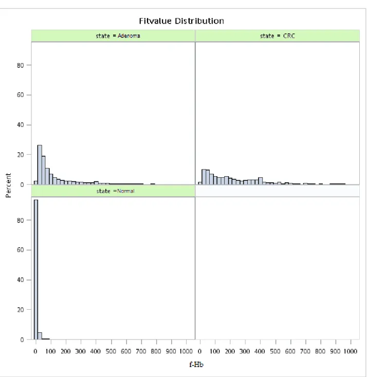
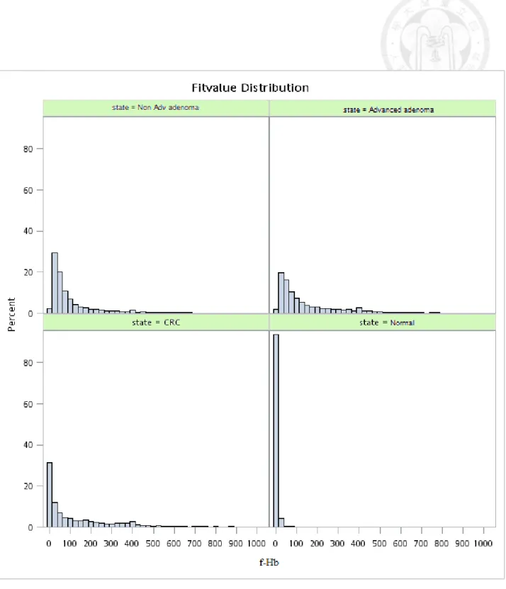
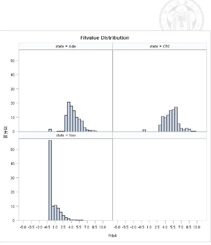
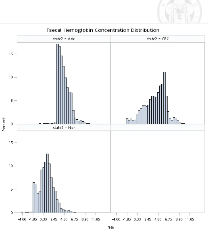
Figure 5.1.1 Histogram of original f-Hb by three disease statuses (normal, adenoma, and colorectal cancer)... 45 Figure 5.1.2 Histogram of original f-Hb by four disease statuses (normal, non-advanced
adenoma, and advanced adenoma, and colorectal cancer)... 46 Figure 5.1.3 Histogram of ln(f-Hb) (adding 0.5 unit to the right) by disease status
before IC interpolation... 47 Figure 5.1.4 Histogram of ln(f-Hb) (excluding undetected cases) by disease status
before IC interpolation... 48 Figure 5.1.5 Histogram of ln(f-Hb) (adding 0.5 unit to the right) by disease status after
IC interpolation... 49 Figure 5.1.6 Histogram of ln(f-Hb) (excluding undetected cases) by disease status after
IC interpolation... 50 Figure 5.2.1 Cumulative distribution of f-Hb by different states before IC
interpolation... 51 Figure 5.2.2 Cumulative distribution curve of f-Hb by different states after IC
interpolation... 52
Figure 5.2.3 Cumulative distribution curve of f-Hb among age groups of cancer patients... 53 Figure 5.2.4 Cumulative distribution curve of f-Hb among age groups in adenoma
patients... 54 Figure 5.2.5 Cumulative distribution curve of f-Hb among gender groups of cancer
patients... 55 Figure 5.2.6 Cumulative distribution curve of f-Hb among gender groups of adenoma
patients... 56
LIST OF TABLES
Table 2.1 Estimated results of re-analysis of symptom and endoscopy measures of treatments for peptic oesophagitis ... 57 Table 2.2 The results of the probability of symptom score after the movement of n
step ... 57 Table 2.3 The results of ruin probabilities with different absorbing
states ... 58 Table 2.4 Estimated results of limiting equilibrium distribution (𝜋𝑘) with reflecting
barriers (state 0 and state 6) on symptomatic scores example ... 58 Table 2.5 The results on the estimates of random walk model parameters (with standard
errors), and log-likelihood for bacitracin and vancomycin treatment groups ... 59 Table 3.1 The descriptive results of f-Hb by disease status and other characteristics of
visits (screens) for each individual ... 60 Table 3.2 Basic characteristics table of f-Hb after adding the value of f-Hb interval
cancer with interpolation ... 61 Table 5.1.1 Interval cancer frequency in all repeated measures ... 62 Table 5.1.2 The results of ANOVA table ... 63
Table 5.1.3 The non-parametric analysis of f-Hb across three disease status ... 63 Table 5.2.1 The estimated hazard ratio of reaching f-Hb using Cox proportional hazards
regression model ... 64 Table 5.2.2 The estimated hazard ratio of reaching f-Hb using the Accelerated failure
time model ... 65 Table 5.3.1 Number of jumps distribution among states ... 66 Table 5.3.2 Step distribution of f-Hb among state ... 66 Table 5.3.3 The estimated parameters on the use of random walk model assuming
normal approximation ... 67 Table 5.3.4 Estimated regression coefficients and their 95% Cis with the random walk
regression model considering three disease statuses, normal, colorectal adenoma, and colorectal cancer ... 68 Table 5.3.5 Estimated forward (p) and backward (q) probability, the odds ratio of p/q,
ruin probability, and the expected steps based on the estimated parameters from Table 5.3.4 ... 68 Table 5.3.6 Estimated regression coefficients and their 95% Cis with the random walk
regression model considering four disease statuses, normal, colorectal
non-advanced adenoma, advanced adenoma, and colorectal cancer ... 69 Table 5.3.7 Estimated forward (p) and backward (q) probability, the odds ratio of p/q,
ruin probability, and the expected steps based on the estimated parameters from Table 5.3.6 ... 69 Table 5.3.8 Estimated regression coefficients and their 95% Cis with the random walk
regression model considering four disease statuses, normal, colorectal adenoma, screen-detected colorectal cancer (SDC), and interval cancer (IC)... 70 Table 5.3.9 Estimated forward (p) and backward (q) probability, the odds ratio of p/q,
ruin probability, and the expected steps based on the estimated parameters from Table 5.3.8 ... 70 Table 5.3.10 Estimated regression coefficients and their 95% Cis with the random walk
regression model considering three disease statuses, normal, colorectal adenoma, and colorectal cancer with two logistic regression models considering forward (p), backward(q), and no movement (r) ... 71 Table 5.3.11 Estimated forward (p), backward (q) probability, staying probability (r) the
odds ratio of p/q, ruin probability, and the expected steps based on the estimated parameters from Table 5.3.10 ... 71
Table 5.3.12 Estimated regression coefficients and their 95% Cis with the random walk regression model considering four disease statuses, normal, colorectal non-advanced adenoma, colorectal advanced adenoma, and colorectal cancer two logistic regression models considering forward (p), backward(q), and no movement (r) ... 72 Table 5.3.13 Estimated forward (p), backward (q) probability, staying probability (r) the
odds ratio of p/q, ruin probability, and the expected steps based on the estimated parameters from Table 5.3.12 ... 72 Table 5.3.14 Estimated regression coefficients and their 95% Cis with the random walk
regression model considering four disease statuses, normal, colorectal adenoma, screen-detected colorectal cancer (SDC), and interval cancer (IC) with two logistic regression models considering forward (p), backward(q), and no movement (r) ... 73 Table 5.3.15 Estimated forward (p), backward (q) probability, staying probability (r) the
odds ratio of p/q, ruin probability, and the expected steps based on the estimated parameters from Table 5.3.14 ... 73 Table 5.3.16 Estimated regression coefficients and their 95% Cis with the random walk
regression model considering three disease statuses, normal, colorectal
adenoma, and colorectal cancer based on all detection modes (including prevalent screen) ... 74 Table 5.3.17 Estimated forward (p) and backward (q) probability, the odds ratio of p/q,
ruin probability, and the expected steps based on the estimated parameters from Table 5.3.16 ... 74 Table 5.3.18 Estimated regression coefficients and their 95% Cis with the random walk
regression model considering four disease statuses, normal, colorectal non-advanced adenoma, advanced adenoma, and colorectal cancer based on all detection modes (including prevalent screen) ... 75 Table 5.3.19 Estimated forward (p) and backward (q) probability, the odds ratio of p/q,
ruin probability, and the expected steps based on the estimated parameters from Table 5.3.18 ... 75 Table 5.3.20 Estimated regression coefficients and their 95% Cis with the random walk
regression model considering three disease statuses, normal, colorectal adenoma, screen-detected colorectal cancer (SDC), and interval cancer (IC) (including prevalent screen) ... 76
Table 5.3.21 Estimated forward (p) and backward (q) probability, the odds ratio of p/q, ruin probability, and the expected steps based on the estimated parameters from Table 5.3.20 ... 76
Table 5.3.22 Estimated regression coefficients and their 95% Cis with the random walk regression model considering three disease statuses, normal, colorectal adenoma, colorectal cancer (CRC), besides that, making allowance for gender (covariate) ... 77 Table 5.3.23 Estimated forward (p) and backward (q) probability, the odds ratio of p/q,
ruin probability, and the expected steps based on the estimated parameters from Table 5.3.22 ... 77 Table 5.3.24 Estimated regression coefficients and their 95% Cis with the random walk
regression model considering three disease statuses, normal, colorectal adenoma, colorectal cancer (CRC), besides that, taking gender as covariate (including prevalence screen) ... 78 Table 5.3.25 Estimated forward (p) and backward (q) probability, the odds ratio of p/q,
ruin probability, and the expected steps based on the estimated parameters from Table 5.3.24 ... 78
I. Introduction
Modelling ordinal data on quantitative biomarker such as fecal hemoglobin concentration (f-Hb) is very intractable partly because of correlated measurements and partly because of incomplete information (censoring and truncation) problem. In addition, absorption barrier (the upper limit value) also adds to the complexity of such a kind of data.
Very few studies have been conducted before to deal with these statistical issues.
One of studies using a random walk model has been conducted to assess the dynamics of score after the administration of endoscopy (Hopper & Young, 1988). However, this study has not evaluated the questions with a formal assessment of such a dynamic ordinal data using the theory of random walk model to report the drift of outcome with unrestricted barrier and the ruin probability with gambler’s algorithm (Cox & Miller, 1965).
We are motivated by the recent research on fecal immunological test (FIT) that is widely used in population-based screening for early detection of colorectal cancer and effective in reducing mortality. The application of FIT has extended from qualitative test to quantitative test based on faecal hemoglobin (f-Hb) concentration. The former is to set a cutoff to classify the participants into positive and negative ones. The latter is to make use of quantitative f-Hb from 0 to upper limit of f-Hb concentration. The recent
researches have also demonstrated the quantitative use of baseline faecal hemoglobin (f-Hb) concentration for predicting incident colorectal neoplasia (Chen, Yen, Chiu, Liao,
& Chen, 2011; Chen et al., 2013) and also colorectal cancer mortality (Chen et al., 2013).
These findings have raised the interest of using quantitative faecal hemoglobin as an ordinal outcome to compare three groups of the underlying population, consisting of free of CRC neoplasia, colorectal adenoma, and colorectal cancer. However, modelling ordinal data such as f-Hb is not straightforward as the distribution is by no means normal distribution and fraught with considerable heterogeneity, including the extreme right values of f-Hb, the outliers of the distribution, and the extreme left undetectable f-Hb that can be treated as left-censored value. To tackle these issues, we treat the order of f-Hb as the outcome of time to event with ranking statistics and apply a Cox proportional hazards regression model to model the difference of f-Hb across three groups (free of CRC neoplasia, colorectal adenoma, and colorectal cancer) with adjustment for other possible covariates.
The first aim of this thesis was to first assess the value of f-Hb across three groups classified by the status of colorectal neoplasia, normal, colorectal adenoma, and colorectal cancer based on a Cox proportional hazards regression model making
interval cancer. The second major aim of this thesis was to apply the random walk model to quantify the dynamic change of f-Hb considering the absorbing barriers because of occurrence of colorectal adenoma and colorectal cancer.
II. Literature Review 2.1 Theory of Random Walk Model
The random walk is a stochastic process in discrete time. Define a simple random walk as fallow: each jump is +1 with probability p, -1 with probability q, and 0 (no jump) with the probability 1-p-q .
That is,
𝑝𝑖𝑗 = {
𝑝 𝑞 1 − 𝑝 − 𝑞
𝑖𝑓 𝑗 = 𝑖 + 1 𝑖𝑓 𝑗 = 𝑖 − 1
𝑖𝑓 𝑗 = 𝑖 (2.1.1)
, with 𝑝𝑖𝑗 = 𝑃𝑟 {𝑋𝑛 = 𝑗|𝑋𝑛−1 = 𝑖}. Where Xn is the position immediately after n jumps, i.e. at time n, Xn = X0+ Z1+ Z2+ ⋯ + Zn, Zi is the moves of in 𝑖th jump and {𝑍𝑖} is a sequence of independently and identically distributed random variables.
There are several types of random walk model that are described as follows.
(1) Unrestricted
We suppose the particle starts at the origin. Also, we assume at time n, the particle reaches the point k. Thus, it has to make 𝑟1 positive jumps, 𝑟2 negative jumps, and 𝑟3
zero jumps. Hence, we have 𝑃𝑟{𝑋𝑛 = 𝑘} = ∑𝑟 𝑛!
1!𝑟2!𝑟3!𝑝𝑟1(1 − 𝑝 − 𝑞)𝑟3𝑞𝑟2 (2.1.2),
over the value of 𝑟, 𝑟 and 𝑟 satisfying 𝑟 − 𝑟 = 𝑘 and n = 𝑟 + 𝑟 + 𝑟 .
distributed with mean 𝑛𝜇 and variance 𝑛𝜎2, with μ= p − q and 𝜎2 = 𝑝 + 𝑞 − (𝑝 − 𝑞)2. Thus, we can have an approximation equation
P(j ≤ 𝑋𝑛 ≤ k) ≅ Φ (𝑘+𝑐−𝑛𝜇
𝜎√𝑛 ) − Φ (𝑗−𝑐−𝑛𝜇
𝜎√𝑛 ) (2.1.3), c=1/2 or c=1 according to the following condition: p + q < 1 or p + q = 1.
(2) Two Absorbing Barriers
Suppose the particle ceases when it reaches either – 𝑏 or 𝑎 (𝑎, 𝑏 > 0). We say that absorption occurs at state 𝑎 (or state – 𝑏). Define 𝑓𝑗𝑎(𝑛) as the probability that the particle is absorbed at a at exactly time n. 𝑓𝑗𝑎(𝑛) is also the probability that an
unrestricted particles, that is,
𝑓𝑗𝑎(𝑛) = 𝑃(−𝑏 < 𝑋1 < 𝑎, … , −𝑏 < 𝑋𝑛−1 < 𝑎, 𝑋𝑛 = 𝑎|𝑋0 = 𝑗) ,
n = 1,2, … (2.1.4), with the initial value condition 𝑋0= 𝑗 when n=0.
Next, we can use the generating function
𝐹𝑗𝑎(𝑠) = ∑∞𝑛=0𝑓𝑗𝑎(𝑛)𝑠𝑛 = 𝐹𝑗(𝑠) (2.1.5),
after the substitution of a trial solution, 𝐹𝑗(𝑠) = 𝜆𝑗, the two solutions are
𝜆1(𝑠), 𝜆1(𝑠) =1−𝑠(1−𝑝−𝑞)±[{1−𝑠(1−𝑝−𝑞)}2−4𝑝𝑞𝑠2]1⁄2
2𝑝𝑠 (2.1.6),
and
𝜆1 =𝑞
𝑝 > 𝜆2 = 1 (𝑝 < 𝑞),
𝜆1 = 1 > 𝜆2 = 𝑞
𝑝 (𝑝 > 𝑞), (2.1.7) 𝜆1 = 1 = 𝜆2 (p = q).
Ruining probability then can be calculated by
𝐹𝑗𝑎(𝑠) ={𝜆{𝜆1(𝑠)}𝑗+𝑏−{𝜆2(𝑠)}𝑗+𝑏
1(𝑠)}𝑎+𝑏−{𝜆2(𝑠)}𝑎+𝑏 (2.1.8), set s=1 and let the particle starts at origin then
P(absorption occurs at a) = 𝐹0𝑎(1) = 1−(
𝑞 𝑝)𝑏
1−(𝑞𝑝)𝑎+𝑏 (2.1.9) and P(absorption occurs at − b) = 𝐹0,−𝑏(1) = 1 − 𝐹0𝑎(1). From the formula derived in the Cox and Miller (1965), denote N as the time to absorption, we have the probability distribution of N
P(N = n) = 𝑓0𝑎(𝑛)+ 𝑓0,−𝑏(𝑛) (2.1.10), and
its generating function
E(𝑠𝑁) = 𝐹0𝑎(𝑠) + 𝐹0,−𝑏(𝑠) (2.1.11).
From the Wald’s identity, the expected number of steps to absorption is
E(N) = {
(𝑎+𝑏)−𝑎𝑒𝜃0𝑏−𝑏𝑒𝜃0𝑎
𝑒−𝜃0𝑎−𝑒𝜃0𝑏 (𝜇 ≠ 0)
𝑎𝑏
𝜇𝜎2 (𝜇 = 0) (2.1.12), 𝜃0 = 2𝜇 𝜎⁄ if the steps follow normal distribution. 2
(3) Two Reflecting Barriers
Suppose the particle starts in the state j and that the state 0 and state a (a>0) are reflecting barriers. Suppose we have 𝑋0 = 𝑗, and
𝑋𝑛 = {𝑋𝑛−1+ 𝑍𝑛 𝑎 0
(2.1.13).
Let 𝑝𝑗𝑘(𝑛) be the probability that the particle occupies the state k at time n having started in the state j. Assume there is a limiting equilibrium distribution of the state occupation probabilities the we have as n → ∞, 𝑝𝑗𝑘(𝑛) → 𝜋𝑘 (k=0,1,…,a). Hence we
obtain the truncated geometric distribution 𝜋𝑘 = 1−𝑝 𝑞⁄
1−𝑝 𝑞⁄ 𝑎+1(𝑝𝑞)𝑘 (k = 0, … , a) (2.1.14).
2.2 Re-analysis of Hopper et al study
As mentioned earlier, one of important papers that applies a random walk model for evaluating clinical trials involving serial observations. In a clinical trial, when the status of patients during and after treatment is recorded, analysis of such information will be more convincing. Applications of semi-Markov models have been restricted to diseases with no reverse transitions. The methods of non-parametric inference for these compartmental processes were based on the martingale theory through counting processes.
The alternative is to use the simple random walk that is a stochastic process in discrete time and can be used to deal with the cases where the multistate aspect of disease status may be summarized by an ordinal measure on which patients may improve or regress throughout the clinical trial. With a numerical maximization routine, this method can provide a suitable statistical inference about the efficacy of different treatment regimes. The random walk model was applied to re-analyze the data on two examples.
(1) Example 1: Symptom and endoscopy measures of treatments for peptic oesophagitis
A double-blind trial was conducted on 59 patients with peptic oesophagitis, the goal is to study the efficacy of two treatments (30 controls, 29 Pyrogastone). Scores were recorded on a six-point scale, and recorded at the same epochs (endoscopy scores:
4 weeks for 3 times; symptomatic scores: 2 weeks
for 5 times).
Table 2.1gives the estimate of two scores.
The authors used the two logistic models to estimate the change of these two scores, and chosen the most fitted one with log-likelihood.
In the endoscopy scores case, they estimated r=0 in control group.
Here the re-estimation using the unrestricted normal approximation gives the following estimates: μ= −0.249 and 𝜎2 = 0.227 for case group in symptomatic scores, and μ= −0.162 and 𝜎2 = 0.176 for the control group.
We also calculated the probability P(𝑋6< 0) = Φ (0+0.5−6×(−0.249) 0.227×√6 ) = Φ(3.59) = 0.9998, P(𝑋6 < −0.5) = Φ (−0.5+0.5−6×(−0.249)
0.227×√6 ) = Φ(2.69) = 0.9964.
Table 2.2 shows the results of the probability P(𝑋𝑛 < −0.5).
Regarding the application to absorbing barriers on symptomatic scores example, we can obtain the ruin probability of different start position j, from 0 to 6 as absorbing state. The ruin probabilities are given in Table 2.3.
For the application on reflecting barriers (state 0 and state 6) on symptomatic scores example, we can obtain the limiting equilibrium distribution 𝜋𝑘 given in Table 2.4.
(2) Example 2: Stool frequency as a measure of treatment for colitis
A randomized double-blind trial compared the effect of two drug treatments, bacitracin or vancomycin. Stool frequencies were recorded on eight successive days for 18 patients in each treatment group, and were categorized into 10 levels (level 1 as an absorbing barrier).
From day 0 to day 7, the mean improvement in bacitracin was 2.73±5 0.56 levels, compared to 3.61 ± 0.38 on vancomycin, (P > 0.20).
Table 2.5 shows the estimates of random walk model parameters (with standard errors), and log-likelihood, for bacitracin and vancomycin treatment groups using stool frequency level data.
The results of analysis with the random walk suggested that patients in the bacitracin group show only 58 percent (comparison of E-values) of the improvement in resolution of diarrhoea. The fit of the four models could have different suggestion, while the changes in log-likelihood were not significant. Thus the inference of this example
It should be noted that very few literatures proposed the random walk model to elucidate the dynamics of such an ordinal data like quality of life. Even the paper proposed the random walk model for dealing with the drift of probabilities. There is lacking of formal assessment of computing the ruin probability for reaching the absorbing barrier and the expected steps (time) taken for reach the boundary of the best improved and the worst unimproved states, which will be my major goal of my thesis.
III. Materials Data on Colorectal Cancer Screening Data
Data we used here are derived from the Taiwanese Nationwide Colorectal Cancer Screening Program using fecal immunochemical test (FIT) as a tool. Details on the planning and implementation of the screening program were reported elsewhere (Chiu et al., 2015). Briefly, the nationwide screening program launched in 2004 was provided to residences of Taiwan aged between 50 to 69 years with a two-year screening interval.
The target population consisted of a residency of 5417699 subjects with a staggered entry with the goal of 20% coverage rate set for the initial 5 years. During the study period between January 1, 2004 and December 31, 2009, there were 1160895 attendees with a coverage rate of 21.4% and a repeat screening rate of 28.3%. The fecal hemoglobin concentration of attended were detected by the OC Sensor method by using two brands of commercial kits. A positive test was defined for the given test and those with positive result were referred for confirmatory diagnosis using colonoscopy as a major method. Individual information such as sex, age, family history, and the outcomes of colorectal neoplasm derived from the report confirmatory diagnosis and cancer registry including non-advance adenoma, advanced adenoma (defied as large than 10mm or with villous component) and colorectal cancer were also collected.
method for the measurement of fecal hemoglobin were excluded from analysis. The basic characteristics of demographic distribution are listed in Table 3.1 and Table 3.2.The dataset consist of 1031314 screenees and 1265305 repeated measures used for the following analysis.
IV. Methodology
In the thesis, we present analysis of fecal hemoglobin (f-Hb) concentration from the application of conventional statistical approach to the development of new random walk model to demonstrate how f-Hb concentration was heterogeneous with three categories of colorectal neoplasia including normal, adenoma (including non-advanced adenoma and advanced adenoma) and colorectal cancer.
4.1. One-way analysis of variance
Instead of treating the disease status of colorectal neoplasia as the outcome, we treat f-Hb as the outcome of interest and the disease status as the independent variable and test the difference in f-Hb across three categories of disease status with the traditional statistical method, one-way analysis of variance. The null hypothesis is set by
H0: 0 = 1 =2
where 0, 1, 2 represent the mean value of normal, colorectal adenoma, and colorectal
cancer. The drawback of using one-way ANOVA is that the result is easily affected by the tail distribution of extreme value.
4.2. Survival Analysis for fecal hemoglobin concentration
It is very interesting in the thesis to consider f-Hb concentration as the ranking data that permits us to consider the use of survival analysis to assess the difference of f-Hb across three or four disease groups with the adjustment for other covariates.
4.2.1 Kaplan-Meyer Method
We therefore first applied the conventional nonparametric method, the Kaplan-Meyer method, to evaluate whether there are differences between colorectal neoplasms, followed by deriving the cumulative distribution curve of f-Hb among different states.
4.2.2 Cox Proportional Hazards Regression Model
Second, we treated the f-Hb of each screenee as the time to event and the disease status as a covariate in Cox proportional hazards regression model. In contrast to survival time, the smaller the f-Hb, the higher the hazard ratio and the lower the risk for developing colorectal neoplasm. By using the method of ties proposed by Breslow (1974), we can deal with the problem of left censoring data with ties resulting from the undetectable f-Hb level.
The reason here that we were not using the exact method for handling the ties was because the population screens cohort contents millions participants, and the sample size was too large for using the exact method. By asymptotic property, the method of ties proposed by Breslow would be expected to be the same as the exact method.
The maximum likelihood estimator of hazard λ0 in terms of β is given at the same f-Hb concentration (denote fi) by
λ̂ = mi i
((fi− fi−1) ∑i∈Riexp(β′Zi))
⁄ (4.2.1) ,
where mi is the number of screenees at fi while Ri is the set of screenees who were not withdrawn between (0, fi ), i.e. whose fi higher then fi-1. Zi here denoted the
covariates we used. The underlying cumulative distribution is estimated by F̂(fi) = ∏ (1 − m𝑙i=1 i∙ ln ∑𝑖∈Riexp(β′Z𝑙)) (4.2.2).
Hence the log-likelihood function would be
ln(L(β)) = ∑ (βki=1 ′si− mi∙ ln ∑i∈Riexp(β′Zi)) (4.2.3) ,
where si is the sum of Zi over the number at fi .
Besides, in order to take into account the correlation as a result of repeated screen in population-based screening, we used the method proposed by Lin and Wei (1989), and requested the robust sandwich estimate for the covariance matrix.
4.2.3 Interval Cancers censored at f-Hb
Because interval cancer patients did not have information on f-Hb when diagnosed, which is defined as the censored data, we computed the faecal hemoglobin concentration of interval cancer cases from random samples of the prevalence screen-detected cancer cases and subsequent screen-detected cancer cases by the stratum of gender and age using the cold-deck method, one of conventional methods for dealing with missing data (Rubin, 1987).
4.3. Random Walk Model
It should be noted that although the equation (2.2.1) can be thought to delineate the random process of the dynamic change of f-Hb, the empirical data as indicated in the section of material do not permit us to directly apply this equation to get the estimate of random sum. Most of repeated screens only included two rounds of screen. Based on Markov property, we assume the change of f-Hb from f-Hb at baseline (measured at first screen, i.e. initial location) after n step for each one screenee is equivalent to n jumps based on any of the change of f-Hb between the value of two successive screens (including first screen and second screen) within the same individual or across individual. By using this assumption, define three possibilities of the change among n jumps denoted by the random variable X where X=1, -1, and 0 represent forward movement, backward movement, and no movement to depict the change of f-Hb between (j-1) th and j th screen. The forward (p), backward probability (q), and no movement (r=1-p-q) of drift are defined by by
{
p , if fHbj− fHbj−1> 0 (move forward) q , if fHbj− fHbj−1< 0(𝑚𝑜𝑣𝑒 𝑏𝑎𝑐𝑘𝑤𝑎𝑟𝑑)
r , fHbj− fHbj−1 = 0 (no movement)
(4.2.4)
.
The random variable X among n jumps follows a multinomial distribution denoted as: X~Multinomial(n, p, q).
4.3.1 Unrestricted Random Walk Model
Supposed that sample size (n) is large enough, with the asymptotic property, we proposed to use the normal distribution as the limiting distribution of Xn when estimating the forward and backward probability.
Xn→ Normal(nμ, nσ a 2) (4.2.5) , with μ= p − q and σ2 = 𝑝 + 𝑞 − (𝑝 − 𝑞)2.
Again, we assumed the steps have identical and independent distribution, hence the step of jth jump ( Xj ) follows normal distribution with mean μ, variance σ2.
The likelihood function is
L = ∏ 1
√2πσ2exp (−(Xj− μ)2 2σ2 )
n
j=1
(4.2.6) ,
and the log-likelihood function is
ln(L) = ∑ −1
2ln(2πσ2) −(Xj− μ)2 2σ2
j
(4.2.7) ,
where n isthe number of jumps.
When analysis, we classified the screenees into three groups by their disease statuses: cancer, adenoma and normal.
4.3.2 Random Walk Logistic Regression Model
The ith jump between jth and (j+1)th screen is denoted by the random variable Xj,
Xj = {
1 , if fHbj− fHbj−1 > 0 0 , if fHbj− fHbj−1 = 0
−1 , if fHbj− fHbj−1< 0
(4.2.8)
Again, X~Multinomial(n, p, q)
To model the effect of disease status on the probabilities of movement, we proposed the generalized logistic regression model for estimating the forward, backward, and no movement. We treated the disease status as a covariate that is incorporated into the generalized logistic regression model, through which we can model the moving probabilities among different states in the same time.
Generalized logistic regression model:
logit(𝑝𝑖) = 𝑙𝑜𝑔 (𝑝𝑖⁄1 − 𝑝𝑖)
= 𝛼0+ 𝛼1∙ 𝑆𝐷𝐶𝑖 + 𝛼2∙ 𝐴𝑑𝑣𝑎𝑑𝑒𝑛𝑜𝑚𝑎𝑖+ 𝛼3 ∙ 𝑁𝑜𝑛𝑎𝑑𝑣𝑑𝑒𝑛𝑜𝑚𝑎𝑖+ 𝛼4
∙ 𝐼𝐶 (4.2.9), logit(𝑞𝑖) = 𝑙𝑜𝑔 (𝑞𝑖⁄1 − 𝑞𝑖)
= 𝛽0+ 𝛽1∙ 𝑆𝐷𝐶𝑖+ 𝛽2∙ 𝐴𝑑𝑣𝑎𝑑𝑒𝑛𝑜𝑚𝑎𝑖 + 𝛽3∙ 𝑁𝑜𝑛𝑎𝑑𝑣𝑑𝑒𝑛𝑜𝑚𝑎𝑖 + 𝛽4
∙ 𝐼𝐶 (4.2.10),
To simplify the generalized logistic regression model, we proposed six
(i) Combine adenoma group and also the cancer group, that is, let α2 = α3, and α1 = α4.
(ii) Combine cancer group, let α1 = α4. (iii) Combine adenoma group, let α2 = α3.
(iv) Combine adenoma group and also the cancer group, that is, let α2 = α3, and α1 = α4 , and estimates parameters by the two logistic regression models.
(v) Combine the cancer group, let α1 = α4 , and estimates parameters by the two logistic regression models.
(vi) Combine the adenoma group, let α2 = α3 , and estimates parameters by the two logistic regression model.
In the model (i), (ii), and (iii), we combined q and r into q and did estimation based only on the first logistic regression model (4.2.9). In the model (iv), (v), and (vi) we used both regression models (4.2.9) and (4.2.10) and then estimated p, q, and r by different states.
In addition to the analysis of data on screenees who had participated more than one time, we also considered including data on prevalent screenees (who participated in screening once only).
In the prevalence case, we assume who diagnosed as cancer or adenoma would move forward, and those who had screening results as normal cases would
either stay on or move backward. Thus we can define the steps of prevalence cases, Xi0= {1 , if the ith prevalence case was cancer or adenoma
0 , if the ith prevalence case was normal (4.2.11) .
Noted in the prevalent screen, there are absence of interval cancers. As the results show no movement probability (r) for cancer and adenoma group is relative low, we only used the same logistic regression model (4.2.9) , and set q=1-p in the following analysis
We have three scenarios when including prevalent cases.
(i) Combine adenoma group and the cancer group, that is, let α2 = α3, and α1 = α4.
(ii) Combine cancer group, let α1 = α4. (iii) Combine adenoma group, let α1 = α4,
After setting up the logistic model for prevalent cases, we can define the
As regards the estimates based on only the regression model (4.2.9), we have (SDC) p1 = exp(𝛼0+ 𝛼1)
1 + exp(𝛼0+ 𝛼1) (4.2.12), (Adv adenoma) p2 = exp(𝛼0+ 𝛼2)
1 + exp(𝛼0+ 𝛼2) (4.2.13) , (Non Adv adenoma) p3 = exp (𝛼0+ 𝛼3)
1 + exp (𝛼0+ 𝛼3) (4.2.14), (IC) p4 = exp (𝛼0+ 𝛼4)
1 + exp (𝛼0+ 𝛼4) (4.2.15), (Normal) p5 = exp (𝛼0)
1 + exp (𝛼0) (4.2.16), and qi = 1 − pi , i = 1,2,3,4,5 (4.2.17).
Regarding the estimates based on both regression models (4.2.9) and (4.2.10), we
have
(SDC) p1 = exp(𝛼0+ 𝛼1)
1 + exp(𝛼0+ 𝛼1) + exp(𝛽0+ 𝛽1) , q1 = exp (𝛽0+ 𝛽1)
1 + exp (𝛼0+ 𝛼1) + exp (𝛽0+ 𝛽1) (4.2.18), (Adv adenoma) p2 = exp(𝛼0 + 𝛼2)
1 + exp(𝛼0+ 𝛼2) + exp(𝛽0+ 𝛽2) , q2 = exp (𝛽0+ 𝛽2)
1 + exp (𝛼0+ 𝛼2) + exp (𝛽0+ 𝛽2) (4.2.19) (NonAdv adenoma) p3 = exp(𝛼0+ 𝛼3)
1 + exp(𝛼0+ 𝛼3) + exp(𝛽0+ 𝛽3) , q3 = exp (𝛽0+ 𝛽3)
1 + exp (𝛼0+ 𝛼3) + exp (𝛽0+ 𝛽3) (4.2.20), (IC) p4 = exp(𝛼0+ 𝛼4)
1 + exp(𝛼0+ 𝛼4) + exp(𝛽0+ 𝛽4) , q4 = exp (𝛽0+ 𝛽4)
1 + exp (𝛼0+ 𝛼4) + exp (𝛽0+ 𝛽4) (4.2.21), (Normal) p5 = exp(𝛼0)
1 + exp(𝛼0) + exp(𝛽0) ,
q5 = exp (𝛽0)
1 + exp (𝛼0) + exp (𝛽0) (4.2.22), and ri = 1 − pi− qi , i = 1,2,3,4,5 (4.2.23).
Then we can have the likelihood function given k screenee:
for analyses based only on (4.2.9) and also based on (4.2.9) and (4.2.10). Assuming the probabilities applied to first screen are the same as the change of f-Hb at successive screens as indicated in the equation (4.2.4). The likelihood function based on the data on first screen is given as follows.
L = ∑ ∑ 𝑝∑ 𝑥1𝑖∙ 𝑞∑ 𝑥2𝑖+∑ 𝑥3𝑖
n
j=1 k
𝑖=1
(4.2.24),
for analyses based on (4.2.9) and (4.2.10),
L = ∑ ∑ 𝑝∑ 𝑥1𝑖𝑗 ∙ 𝑞∑ 𝑥2𝑖𝑗 ∙ 𝑟∑ 𝑥3𝑖𝑗
ni
j=0 k
i=1
(4.2.25),
Where
𝑥1𝑖 = {1 , 𝑖𝑓 𝑋𝑖 = 1 0 , 𝑜. 𝑤.
𝑥2𝑖 = {1 , 𝑖𝑓 𝑋𝑖 = −1
0 , 𝑜. 𝑤. (4.2.26), 𝑥3𝑖 = { 1 , 𝑖𝑓 𝑋𝑖 = 0
0 , 𝑜. 𝑤.
The likelihood function for the n jumps of subsequent screens as indicated above was also derived in a similar manner.
With the random walks model and the regression equations we set up, we can estimated the coefficients of variables and calculated the probabilities movement in random walk model.
4.3.3 Gambler’s ruin and expected number of game
After the estimation of the probabilities of movement, we can further apply the gambler’s ruin theorem. The gambler’s ruin problem is the random walks with
absorbing barriers 0 and N. A gambler starts out with x f-hb, and he wins 1 unit with probability p and lose 1 unit with probability q=1-p. The gambler stops when he has a state of 0 or N .
Following the formal derivation of processes for the two absorbing barriers by Cox and Miller (1965), here we use alternative way of deriving the ruin probability.
We are interesting in the computation of probability Vx that the player will be ruined after commencing with x. At the end of the first game (first step analysis), he will has (x+1) if he wins the game with p (Vx+1), or he will has (x-1) if he loses the
game with q (Vx-1). Thus, we have
Vx = qVx−1+ pVx+1 , 0 < 𝑥 < 𝑁 (4.2.27)
p(Vx+1− Vx) = q(Vx+ Vx−1) ,
Vx+1− Vx = q p⁄ (Vx+ Vx−1) .
By recursive method, we have
Vx+1− Vx= (q p⁄ )x(V1− 1) , 0 < 𝑥 < 𝑁 (4.2.28),
Let
Vx− 1 = Vx− V0 = (Vx− Vx−1) + (Vx−1− Vx−2) + ⋯ + (V1− 1)
= {
1 − (q p⁄ )x
1 − (q p⁄ ) (V1− 1) p ≠ q x(V1− 1) p = q
(4.2.29) .
The absorbing barrier leading to 𝑉𝑁 ,
Vx= {
1 −1 − (q p⁄ )x
1 − (q p⁄ )N p ≠ q 1 − x
N p = q
(4.2.30) .
Furthermore, let Dx denote the expected time until a gambler who starts with x, say 1 (f-hb) is ruined.
The boundary conditions are D0=0, DN=0. By first-step analysis,
Dx = q(Dx−1+ 1) + p(Dx+1+ 1) = 1 + qDx−1+ pDx+1 (4.2.31)
p(Dx+1− Dx) = q(Dx− Dx−1) − 1
Let Mx = Dx− Dx−1
pMx+1= qMx−1 (4.2.32)
Again by the recursive method, we have
Mx = (q
p)x−1M1−1 p∑ (q
p)j
x−2
(4.2.33)
Dk= ∑kj=1Mj = ∑kj=1[(qp)jD1−1p∑j−2i=0(qp)j] =
{
1−(q p⁄ )k
1−(q p⁄ ) [D1−p−q1 ] −p−qk (p ≠ q) k(D1− (k − 1)) (p = q)
(4.2.34)
With DN= 0,
D1 = { N
p( 1
1 − (q p⁄ )N) − 1
p − q (p ≠ q) N − 1 (p = q)
(4.2.35)
Thus we can calculate the expected number of game (Dx) until the gambler that starts at $x is ruined.
Dx = {
1 − (q p⁄ )x
1 − (q p⁄ ) [D1− 1
p − q] − x
p − q (p ≠ q) x(N − x) (p = q)
(4.2.36)
V. Results
5.1 One-way analysis of variance
Table 3.1 shows the descriptive results of f-Hb by disease status and other characteristics such as gender, age, family history, and brand type. The similar findings are shown when interval cancer is added (Table 3.2). Table 5.1.1 shows the frequencies of all repeated screens. Figure 5.1.1-5.1.6 shows the distribution of original f-Hb and also the corresponding ones with log transformation. These figures also show the results with and without considering undetectable f-Hb (including 0) in the normal group. The undetectable problem is considered by left censoring with the Breslow tie method in the Cox proportional hazards regression model. It can be seen that the log transformation renders the positive skewed distribution go toward a normal shape.
The analysis of variance for the log transformation of f-Hb (adding 0.5 unit to the right) shows that the difference in the mean value of f-Hb across three groups were statistically significant. (Table 5.1.2, p<0.001, R2=0.142). The similar findings were noted when the non-parametric analysis was performed (Table 5.1.3).
5.2 Cox Proportional Hazards Regression Model
The results of univariable analysis are listed in Table 5.2.1 showing significant differences in the f-Hb concentration between categories of colorectal neoplasm, with disease-free case (normal group) as the reference group, the hazard ratio (HR) of the colorectal cancer group was 0.197 (0.194, 0.20), and the HR of the adenoma group was 0.213 (0.212, 0.215).
The results of multivariable analysis also show that men generally had higher f-Hb concentration than women (HR=0.948, (0.944, 0.951)), the old age group also had higher f-Hb concentration than the young age group. The effect of family history was significant in univariable analysis (HR=1.051, (1.036, 1.067)) but not significant in multivariable analysis (HR=1.012, (0.997, 1.027)). After adjusting for other covariates (gender, age, family history and brand), compared to the normal group, the HR of the cancer group was 0.181 (0.178, 0.184) and the adenoma group was 0.204 (0.202, 0.205). This model clearly clarifies that those who had been diagnosed with colorectal cancer tended to have higher f-Hb level in screening, as the adenoma group does. This indicates that screenee who had higher f-Hb may have higher probability to be diagnosed with disease. Table 5.2.2 shows the similar findings estimated by the accelerated failure time model.
Figures 5.2.1 and 5.2.2 show the cumulative figure with the non-parametric
method for f-Hb. We found the computation of f-Hb for interval cancer with the cold-deck method got the curve corrected (Figure 5.2.1 and Figure 5.2.2). Based on the nonparametric method we can also assess the f-Hb50 of CRC was 142 g Hb/g,
f-Hb50 of adenoma was 66 g Hb/g, and f-Hb50 of normal near 0 g Hb/g. The threshold value was 600 g Hb/g for CRC and 400 g Hb/g for adenoma. (Figure
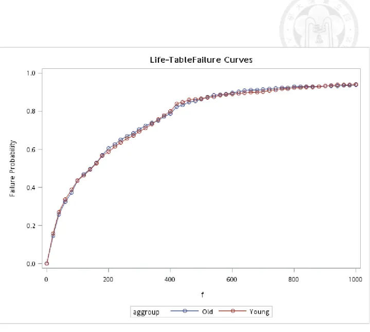
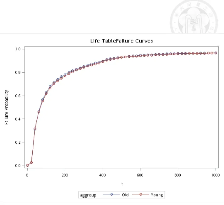
5.2.2). Figures 5.2.3-5.2.5 show the corresponding curves by gender and age groups for cancer. The conspicuous difference was noted in the Figure of adenoma by gender (Figure 5.2.6).
5.3 The Random Walk Model
We used the faecal hemoglobin concentration of screenees as the repeated measures, the f-Hb change from last time over than 0 with probability p, less than 0 with probability q, and the staying probability is r. Tables 5.3.1 and 5.3.2 display the basic distribution of the steps about fecal hemoglobin concentration among all the states.
By assuming the normal distribution of each step and applying the central limit theorem, the unrestricted estimates for three groups are listed in Table 5.3.3. It can be clearly seen that the highest forward probability was noted for the colorectal