Abstract—This paper proposes ElevatorTalk, an elevator development and management system based on an IoT approach called IoTtalk. This system modularizes the software into elevator components so that we can easily develop flexible and scalable car scheduling algorithms. ElevatorTalk consists of three subsystems:
Cars, Scheduler and the Elevator Car Operating (ECO) Panel.
The first two subsystems are used to develop the elevator systems, and the third subsystem is used to receive requests issued by the passengers as well as to generate the request patterns to test the developed algorithms. These three subsystems work in parallel, and communicate with each other through sending and receiving messages. ElevatorTalk can connect to a real elevator system to serve as the elevator management center. It can also emulate existing elevator systems with different car scheduling algorithms.
We propose an intelligent aggressive car scheduling with initial car distribution algorithm (ACSICD) and implement it in ElevatorTalk. Our study indicates that ACSICD has better waiting/travel/journey time performance and/or accuracy than the previous proposed algorithms. We also show that in our approach, the car scheduling decision can be quickly made with 0.2010 ms, and therefore good performance in the time complexity is achieved.
Index Terms—Car scheduling, elevator system, Elevator Car Operating (ECO) Panel, emulator, intelligent, Internet of Things (IoT), sensor, and waiting/travel/journey time.
I. INTRODUCTION
s the population increases, high-rise buildings have mushroomed around the world. Since Werner von Siemens [1] presented the world’s first electric elevator in 1880, this invention has played an indispensable role in tall buildings to carry the passengers and goods. From the viewpoint of a passenger in a tall building, waiting for the elevator car during peak hours is frustrating experience.
Therefore, it is essential that elevator scheduling optimizes the waiting/travel/journey times of the passengers. The elevator group control systems including single-car elevator [8], multi-car elevator [3][4][6][7][9][10][12-20][23][24] and double-decker elevator [20] have been extensively explored in this field [2-24]. In [10], a simulator was developed to study the
Manuscript received Jan. 08, 2019. L. D. Van (e-mail:
[email protected]), Y.-B. Lin (email: [email protected]), T. H. Wu, and Y. C. Lin are with the Dept. of Computer Science, National Chiao Tung University, Hsinchu, 300, Taiwan. This work was supported in part by the MOST 107-2218-E-009-020 and MOST 106-2221-E-009 -028-MY3.
multi-car elevator that consists of more than one car (cabin) in one shaft. Many researchers have applied neural network [2][5][16], fuzzy [4][17], genetic methods [3][6][9][13][18]
and reinforcement learning [15][16] to optimize elevator car scheduling. A good survey of elevator group control can be found in [20]. Some papers have proposed solutions to resolve the elevator car scheduling problems [2-10][12-20][23]. Most recent results have been summarized and compared in [18][20][21]. In this paper, we propose ElevatorTalk system and compare our approach with the previous studies. The originality/contributions of this paper are described as follows.
1) ElevatorTalk system is proposed to modularize the software into elevator components such that the flexible and scalable car scheduling algorithms can be easily developed.
2) ElevatorTalk can connect to a real elevator system to serve as the elevator management center and can emulate existing elevator systems with different car scheduling algorithms.
3) An intelligent aggressive car scheduling with initial car distribution algorithm (ACSICD) is proposed to reduce the waiting/travel/journey time compared with other algorithms.
4) The effects of the variable measured door open delay and fixed door open delay are discussed for accuracy.
The paper is organized as follows. Section II describes the ElevatorTalk architecture. Section III develops a parallel ACSICD implemented in ElevatorTalk. Section IV compares ACSICD with the previously proposed approaches. Section V summarizes our findings.
II. ELEVATORTALK ARCHITECTURE
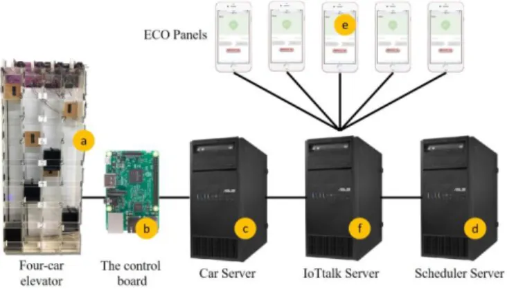
Figure 1 (a) shows a four-car elevator model we built. An Raspberry PI board (Figure 1 (b)) [25] is used to control the motors and doors of the elevator cars. This control board is connected to the Car server (Figure 1 (c)). The cars in the elevator system are driven by the Cars subsystem implemented in the Car server. The Cars subsystem is instructed by the Scheduler subsystem implemented in the Scheduler server (Figure 1 (d)). The Scheduler subsystem reads the requests issued from the Elevator Car Operating (ECO) Panels (Figure 1 (e)). An ECO Panel can be a traditional panel mounted on the wall or a smartphone with the ECO Panel app. The Cars, the Scheduler and the ECO Panel subsystems are implemented as cyber IoT devices in an application-layer IoT device management platform called IoTtalk [26-29] adopting the skills/resources [30-35]. Therefore, the Car server, the
An Intelligent Elevator Development and Management System
Lan-Da Van, IEEE Senior Member, Yi-Bing Lin, IEEE Fellow, Tsung-Han Wu, Yu-Chi Lin
A
Figure 1. The ElevatorTalk hardware architecture.
Scheduler server and the ECO Panels are connected to the IoTtalk server (Figure 1 (f)). IoTtalk allows the user to quickly establish connections and meaningful interactions between IoT devices without concerning the lower layer IoT platforms/protocols (such as AllJoyn [36], oneM2M [37], and so on). IoTtalk manages IoT devices based on a concept called
“device feature” (DF). A DF is a specific input or output
“capability” of an IoT device. For example, an air quality monitoring device has an input device feature (IDF) called the PM2.5 sensor that produces the particulate matter 2.5 measure in μg/m3. A pair of wearable glasses with the optical head-mounted display has the output device feature (ODF) called “Display”. An IoT device is a collection of DFs. In IoTtalk, every IoT device can be partitioned into one input and one output devices. The input device is a subset of the IoT device consisting of the input DFs of that device. Similarly, the output device consists of the output DFs of that device. An IoT device is connected to the IoTtalk server through wired or wireless communications technologies, and network applications are automatically created/re-used at the IoTtalk server for the IoT devices. When the IDFs of the IoT device produce new values, they are sent to the server, and the corresponding network application is executed to take actions, which may produce results to be sent to the ODFs of the same or other IoT devices.
In IoTtalk, the Cars, the Scheduler and the ECO Panel subsystems are cyber devices. In a typical elevator system, there is a physical ECO Panel for each floor and a panel inside every car. In the elevator system, all physical panels are connected to the IoTtalk server through the ECO Panel subsystem. The ECO Panel subsystem represents both the floor panels and the car panels pressed by the passengers to specify the source (the start floors) and the destinations (the target floors). The Scheduler subsystem accepts and handles the requests from the ECO Panel subsystem, and schedules the movement of the cars. Following the instructions of the Scheduler subsystem, the Cars subsystem is in charge of the car operations, such as moving up or down the cars, and opening or closing doors. The Scheduler server, the Car server, the IoTtalk server and the ECO Panel subsystem can be installed in a local server, a private or a public cloud. The physical ECO Panels and the cars/controllers are installed in the building.
IoTtalk provides a friendly graphical user interface (GUI) to specify the ElevatorTalk devices and their connection configurations. In this web-based GUI window, an input device
is represented by an icon placed at the left-hand side of the window (Figure 2 (a), (c), (e)), which consists of smaller icons that represent IDFs (Figure 2 (1)-(4), (9)-(12), and (18)). The IDFs are appended with “-I”. Similarly, an output device is represented by an icon placed at the right-hand side of the window (Figure 2 (b) and (d)), which includes ODF icons (Figure 2 (5)-(8) and (13)-(17)). The ODFs are appended with
“-O”. By connecting the IDFs to the ODFs in the GUI (Joins 1-9), the devices interact with each other without any programing effort. The Cars subsystem controlling 𝑁 cars (𝑁 = 4 in this example) consists of both input and output devices. The input device has 𝑁 IDFs, where 1 ≤ 𝑛 ≤ 𝑁. The IDF Car-n-I (Figure 2 (1)-(4)) provides the motion status of the n-th car. The output device has 𝑁 ODFs, where the ODF Car-n-O (Figure 2 (5)-(8)) accepts the requests for moving the n-th car. Similarly, the Scheduler subsystem consists of both input and output devices. The input device has 𝑁 IDFs, where Car-n-I (Figure 2 (9)-(12)) instructs the n-th car to move. The output device has 𝑁 + 1 ODFs. The Request-O ODF (Figure 2 (13)) receives the passenger requests from the ECO Panel, and the Status-n-O ODF (Figure 2 (14)-(17)) receives the status information of the n-th car. The Panel subsystem has one IDF called Request-I (Figure 2 (18)) to send out the passenger requests.
Figure 2. Configuring ElevatorTalk through the IoTtalk GUI (𝑁 = 4)
III. ELEVATORTALK PROCEDURES AND THE INTELLIGENT AGGRESSIVE
CAR SCHEDULING WITH INITIAL CAR DISTRIBUTION ALGORITHM
(ACSICD)
This section describes the procedures developed by the ElevatorTalk subsystems. Then we propose an intelligent aggressive car schedule algorithm with initial car distribution algorithm (ACSICD) for the elevator system and show how the algorithm is implemented in ElevatorTalk. Specifically, Section III.A implements Procedure Panel for the ECO Panel subsystem (Figure 2 (e)). Sections III.B-III.D elaborate on four procedures ReqArrival, SchCar(n), UpTaskCar(n) and DownTaskCar(n) implemented in the Scheduler subsystem
(Figure 2 (c) and (d)). Section III.E describes Procedures Car(n) for the Cars subsystem (Figure 2 (a) and (b)).
In the current implementation, Procedures Car(n) are implemented as threads in the Car server, which are run in parallel. Similarly, the procedures for the Scheduler subsystem are implemented as independent threads. To describe the ElevatorTalk procedures, the symbols defined in Table 1 are used in this paper.
Table 1. Symbols used in the ElevatorTalk procedures.
Symbol Description 𝐶𝐵 The set of busy cars.
𝑑𝑛 The current moving direction of the n-th car; 𝑑𝑛∈ {𝑈𝑝, 𝐷𝑜𝑤𝑛, 𝐼𝑑𝑙𝑒}.
𝐷𝑚 The moving direction of 𝑟𝑚; 𝐷𝑚∈ {𝑈𝑝, 𝐷𝑜𝑤𝑛} .
𝑓𝑛 The current floor of the n-th car.
𝑓𝑠(𝑚) The start floor of 𝑟𝑚.
𝑓𝑡,𝑟(𝑚, 𝑘) The k-th target floor in 𝑟𝑚, where 1 ≤ 𝑘 ≤ 𝑘𝑚.
𝑓𝑡,𝑐(𝑛, 𝑗) The j-th target floor in the n-th car’s stop list 𝑆𝑡,𝑐(𝑛), where 1 ≤ 𝑗 ≤ 𝑗𝑛.
𝐹 The number of floors in the building.
𝑗𝑛 The number of target floors in 𝑆𝑡,𝑐(𝑛).
𝑘𝑚 The number of target floors in 𝑟𝑚.
𝐿𝑢 The set Uplist of all unhandled 𝑓𝑠(𝑚) , where 𝐷𝑚 is Up.
𝐿𝑑 The set Downlist of all unhandled 𝑓𝑠(𝑚) , where 𝐷𝑚 is Down.
𝑀 The number of requests issued during the observation period.
𝑁 The number of cars in the elevator system.
𝑜𝑛 A flag that indicates if the n-th car should open door or not. 𝑜𝑛∈ {0,1}.
𝑟𝑚 The m-th request from an ECO panel, where 1 ≤ 𝑚 ≤ 𝑀;
𝑟𝑚= ( 𝑓𝑠(𝑚) , 𝐷𝑚 , 𝑆𝑡,𝑟(𝑚) ).
𝑆𝑡,𝑐(𝑛) The set of the target floors to be stopped by the n-th car in the
current moving direction; 𝑆𝑡,𝑐(𝑛) =
{𝑓𝑡,𝑐 (𝑛, 1), 𝑓𝑡,𝑐 (𝑛, 2), … , 𝑓𝑡,𝑐 (𝑛, 𝑗𝑛)}.
𝑆𝑡,𝑟(𝑚) The set of target floors in 𝑟𝑚;
𝑆𝑡,𝑟(𝑚) = {𝑓𝑡,𝑟(𝑚, 1), 𝑓𝑡,𝑟(𝑚, 2), … , 𝑓𝑡,𝑟(𝑚, 𝑘𝑚)}.
𝑡𝑑 The door open delay.
𝑡𝑓 The delay of car moving up/down one floor.
𝑡𝑚 The arrival time of 𝑟𝑚; by default, 𝑡0= 0.
𝜏𝑚 The inter-arrival time between request 𝑟𝑚−1 and 𝑟𝑚, where 𝑟0 is a null request, and 𝜏𝑚= 𝑡𝑚− 𝑡𝑚−1.
𝑡𝑠 The delay between when a request 𝑟𝑚 arrives and when a car opens the door to handle the request.
𝑇𝑚,𝑛 The waiting time of 𝑟𝑚 if it is served by the n-th car.
𝑥𝑛 The number of known stops on the moving path of the n-th car from 𝑓𝑛 to 𝑓𝑠(𝑚). Let 𝐿𝑢,𝑛 be the floors in 𝐿𝑢, where the n-th car stops to pick the passengers. Similarly, let 𝐿𝑑,𝑛 be the floors in 𝐿𝑑, where the n-th car stops to pick the passengers. If 𝑑𝑛= 𝑈𝑝 then 𝑥𝑛= {𝑥| 𝑥 ∈ 𝑆𝑡,𝑐(𝑛) ∪ 𝐿𝑢,𝑛 and 𝑓𝑛≤ 𝑥 ≤ 𝑓𝑠(𝑚)} . If 𝑑𝑛= 𝐷𝑜𝑤𝑛 then 𝑥𝑛= {𝑥| 𝑥 ∈ 𝑆𝑡,𝑐(𝑛) ∪ 𝐿𝑑,𝑛 and 𝑓𝑠(𝑚) ≤ 𝑥 ≤ 𝑓𝑛}.
A. Procedure Panel
The ECO panel subsystem implements Procedure Panel as a thread run on the IoTtalk server. Through the IoTtalk server, the ECO Panel subsystem connects to the physical ECO panels.
When a passenger presses a button of an ECO panel, the instruction is captured by Procedure Panel. Let 𝑟𝑚 be the m-th request issued from a panel, which has the format 𝑟𝑚= ( 𝑓𝑠(𝑚), 𝐷𝑚 , 𝑆𝑡,𝑟(𝑚)), where
𝑓𝑠(𝑚) is the floor from which 𝑟𝑚 is issued,
𝐷𝑚∈ {𝑈𝑝, 𝐷𝑜𝑤𝑛}is the moving direction of 𝑟𝑚, and
𝑆𝑡,𝑟(𝑚) is the set of target floors in 𝑟𝑚.
Both 𝑓𝑠(𝑚) and 𝐷𝑚 are known before the passenger enters the car, and 𝑆𝑡,𝑟(𝑚) is determined after the passenger entered the car. When 𝑟𝑚 arrives, Procedure Panel sends 𝑟𝑚 to the Scheduler subsystem through Join 9 in Figure 2.
In real world, an elevator system operates for a period of time and then is shut down for maintenance. Without loss of generality, we assume that Procedure Panel runs to serve M requests, and then stops for system maintenance. The flowchart is illustrated in Figure 3. At Step P.1, there is no request, and 𝑚 is set to 0 initially. Step P.2 checks if M requests have been served. If so, the service is stopped for maintenance at Step P.5.
Otherwise, wait for the next request at Step P.3. At Step P.4, request 𝑟𝑚 is sent to the Scheduler subsystem for service. We have also implemented a panel emulator that can generate a sequence of M requests to test the elevator system. The flowchart is the same as that in Figure 3 except for Step P.3. In the emulator, Step P.3.2 is replaced by the following three sub-steps.
Step P.3.2. Create the inter-arrival time 𝜏𝑚 by a random number generator RNG() following the Poisson process (note that an arbitrary inter-arrival time distribution as well as trace-driven emulation can be implemented).
Step P.3.3. Invoke function sleep(𝜏𝑚) to wait for a time period 𝜏𝑚.
Step P.3.4. Generate the next request 𝑟𝑚.
Start m 0
P.1
1. m m+1 ; 2. Wait for the next request
Send (rm , m) to Request-O of Scheduler
P.2
P.4
if m < M
Yes
Stop
P.3
P.5
No
Figure 3. Flowchart for Procedure Panel.
B. Procedure ReqArrival
Procedure ReqArrival is implemented as the top priority thread in the Scheduler subsystem, which dispatches all tasks for scheduling. Let 𝐷𝑚 be the moving direction for 𝑟𝑚. Several data structures manipulated at the Scheduler subsystem are initialized by Procedure ReqArrival (Step R.1, Figure 4), where Uplist 𝐿𝑢 is the set of all unhandled 𝑓𝑠(𝑚) with 𝐷𝑚= Up, Downlist 𝐿𝑑 is the set of all unhandled 𝑓𝑠(𝑚) with 𝐷𝑚= 𝐷𝑜𝑤𝑛 , and 𝐶𝐵 is the set of busy cars. Since these data structures are accessed by all threads in the Scheduler subsystem, they must be locked to avoid multiple updates at the same time. At Step R.2, for 1 ≤ 𝑛 ≤ 𝑁, the Scheduler subsystem creates the thread SchCar(n) to handle the request assignment for the n-th car. Step R.3 waits to receive the request (𝑟𝑚, m) issued from the ECO Panel subsystem. If the moving direction of 𝑟𝑚 is Up at Step R.4, then the request is included in 𝐿𝑢 (see Step R.5). Otherwise, the request is included in 𝐿𝑑 (see Step R.6). Then the flow goes to Step R.3 to wait for the arrival of the next request. When the elevator system is turned on, ReqArrival repeatedly executes the loop (see Steps R.3 ~ R.6) until the system is shut down.
Start
1. Lock Acquire ; 2. Lu Ø ; 3. Ld Ø ; 4. CB Ø ; 5. Lock Release
R.1
R.3
R.4
Wait to request (rm , m) from Request-I of Users
1. Lock Acquire ; 2. Lu Lu { fs(m)} ; 3. Lock Release
if Dm = Up Yes No
∪
1. Lock Acquire ; 2. Ld Ld { fs(m)} ; 3. Lock Release
∪
R.5 R.6
for 1 n N : Create SchCar(n)
R.2
Figure 4. Flowchart for Procedure ReqArrival.
C. Procedure SchCar(n)
Procedure SchCar(n) is responsible for scheduling of the n-th car. Figure 5 illustrates the flowchart with two local data structures. The first data structure 𝑑𝑛∈ {𝑈𝑝, 𝐷𝑜𝑤𝑛, 𝐼𝑑𝑙𝑒} is the current moving direction and the second data structure 𝑆𝑡,𝑐(𝑛) = {𝑓𝑡,𝑐 (𝑛, 1), 𝑓𝑡,𝑐 (𝑛, 2), … , 𝑓𝑡,𝑐 (𝑛, 𝑗𝑛)} is the set of the target floors to be stopped by the n-th car in the current moving direction. In 𝑆𝑡,𝑐(𝑛), 𝑓𝑡,𝑐(𝑛, 𝑗) is the j-th target floor in 𝑆𝑡,𝑐(𝑛),
Start
1. dn Idle ; 2. St,c(n) Ø ; 3. Wait to receive (n, fn) from Car-n-I of Cars ; 4. Send (n, 0, Idle) to Car-n-O of Cars ;
S.1
dn = ? dn = Down
dn = Up dn = Idle S.2
DownTaskCar(n) UpTaskCar(n) S.4
S.8
S.6 1. Lock Acquire ; 2. CB CB – {n}
S.7
Lock Acquire
Lock Release S.3
Yes
No
No
No
Yes
Yes
Yes
dn Up;
CB CB {n}
dn Down;
CB CB {n}
dn Down;
CB CB {n} ∪
∪
∪
dn Up;
CB CB {n} ∪
Yes No
S.5
S.9
S.10
S.11
S.13
S.14
S.15
S.16
S.17
No
≥ )
∈
∃
( fu Luandfu fn
if
≤ )
∈
∃
( fd Ldandfd fn
if
) (|L|+|L|
|<α C
|
if B u d
)
∈ <
∃
( fu Luandfu fn
if
)
∈ >
∃
( fd Ldandfd fn
if
ICD S.12
Figure 5. Flowchart for Procedure SchCar(n).
where 1 ≤ 𝑗 ≤ 𝑗𝑛, and 𝑗𝑛= |𝑆𝑡,𝑐(𝑛)|is the number of target floors. At Step S.1, 𝑑𝑛 is set to idle, and 𝑆𝑡,𝑐(𝑛) is empty. The SchCar(n) thread of the Scheduler subsystem and the Car(n) thread of the Cars subsystem must be synchronized.
Specifically, Steps S.1.3 waits to receive the current status (n, 𝑓𝑛) of the n-th car from Car(n), and then Step S.1.4 sends the acknowledgement (n, 0, Idle) to Car(n) to make sure that the connection between these two threads is established. After initialization, SchCar(n) enters a loop. Step S.2 checks if the n-th car is moving. If the car is idle, then Step S.7 checks if the n-th car should serve incoming requests based on the total
number of unhandled requests. Before Step S.7 is executed, Step S.3 locks 𝐶𝐵, 𝐿𝑢 and 𝐿𝑑 to ensure that other threads will not modify these global data structures at the same time. Step S.16 releases the lock and loops back to Step S.2. At Step S.7, the positive value α ≤ 1 is the aggressive factor that specifies how aggressive the elevator wants to serve the passengers. A large α value means that the system aggressively serves the requests with more cars. Specifically, if the number |𝐶𝐵| of busy cars is larger than or equal to α(|𝐿𝑢| + |𝐿𝑑|) then the n-th car will not handle any request and then the function of initial car distribution (ICD) in Step S.12 is executed. According to observations of the traffic patterns in an elevator system, a dynamic approach for stochastic time consistency on big data [38] is used to determine ICD function controls the n-th car to park at the floor which has the largest number of requests in certain periods. For example, in an office building, an idle car will parks at the ground floor in the morning (when people are coming to their office) and parks at the highest floor in the evening (when people are leaving the building). After ICD, the control flow loops back to Step S.2. Otherwise, the car takes care of an unhandled request in one of four cases illustrated in Figure 6.
Case 1 (Steps S.8 and S.13). For a passenger at a floor above the n-th car, if he/she wants to go upward and the car is idle or moving up, then the car moves up to handle the request.
Case 2 (Steps S.9 and S.14). If there is a passenger at a floor below the n-th car, and he/she wants to go downward where the car is idle or moving down, then the car moves down to handle the request.
Case 3 (Steps S.10 and S.15). If there is a passenger at a floor below the n-th car who wants to go upward and the car is idle, then the car moves down to handle the request.
Case 4 (Steps S.11 and S.16). If there is a passenger at a floor above the n-th car, and he/she wants to go downward and the car is idle, then the car moves up to handle the request.
If 𝑑𝑛 is Down at Step S.2, the flow proceeds to Step S.4 that invokes DownTaskCar(n) to handle all moving-down requests (to be elaborated in Section III.D). After all requests for the n-th car have been served, Step S.6 acquires the lock (just like Step S.3) and proceeds to Step S.7 to see if there are new tasks for the n-th car. Similar to Step S.4, if 𝑑𝑛 is Up at Step S.2, then Step S.5 is executed to handle the moving-up requests.
Figure 6. Four cases for the relationship between a car and a request at floors 3 and 5.
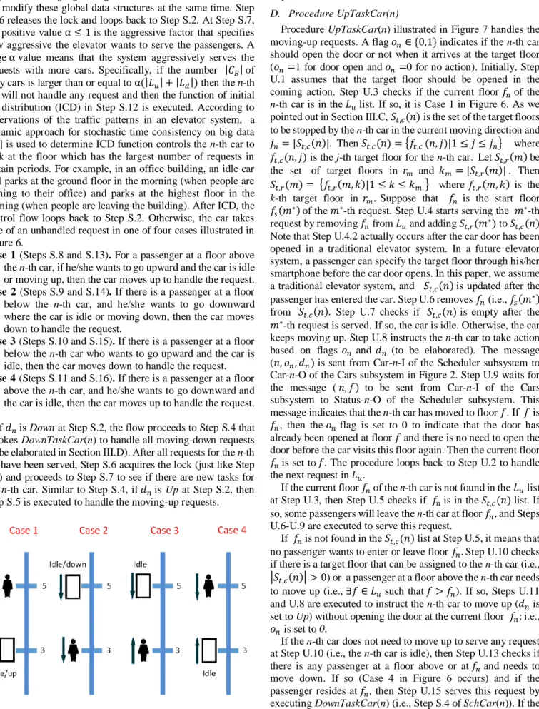
D. Procedure UpTaskCar(n)
Procedure UpTaskCar(n) illustrated in Figure 7 handles the moving-up requests. A flag 𝑜𝑛∈ {0,1} indicates if the n-th car should open the door or not when it arrives at the target floor (𝑜𝑛=1 for door open and 𝑜𝑛=0 for no action). Initially, Step U.1 assumes that the target floor should be opened in the coming action. Step U.3 checks if the current floor 𝑓𝑛 of the n-th car is in the 𝐿𝑢 list. If so, it is Case 1 in Figure 6. As we pointed out in Section Ⅲ.C, 𝑆𝑡,𝑐(𝑛) is the set of the target floors to be stopped by the n-th car in the current moving direction and 𝑗𝑛= |𝑆𝑡,𝑐(𝑛)|. Then 𝑆𝑡,𝑐(𝑛) = {𝑓𝑡,𝑐 (𝑛, 𝑗)|1 ≤ 𝑗 ≤ 𝑗𝑛} where 𝑓𝑡,𝑐(𝑛, 𝑗) is the j-th target floor for the n-th car. Let 𝑆𝑡,𝑟(𝑚) be the set of target floors in 𝑟𝑚 and 𝑘𝑚= |𝑆𝑡,𝑟(𝑚)| . Then 𝑆𝑡,𝑟(𝑚) = {𝑓𝑡,𝑟(𝑚, 𝑘)|1 ≤ 𝑘 ≤ 𝑘𝑚 } where 𝑓𝑡,𝑟(𝑚, 𝑘) is the k-th target floor in 𝑟𝑚. Suppose that 𝑓𝑛 is the start floor 𝑓𝑠(𝑚∗) of the 𝑚∗-th request. Step U.4 starts serving the 𝑚∗-th request by removing 𝑓𝑛 from 𝐿𝑢 and adding 𝑆𝑡,𝑟(𝑚∗) to 𝑆𝑡,𝑐(𝑛).
Note that Step U.4.2 actually occurs after the car door has been opened in a traditional elevator system. In a future elevator system, a passenger can specify the target floor through his/her smartphone before the car door opens. In this paper, we assume a traditional elevator system, and 𝑆𝑡,𝑐(𝑛) is updated after the passenger has entered the car. Step U.6 removes 𝑓𝑛 (i.e., 𝑓𝑠(𝑚∗)) from 𝑆𝑡,𝑐(𝑛). Step U.7 checks if 𝑆𝑡,𝑐(𝑛) is empty after the 𝑚∗-th request is served. If so, the car is idle. Otherwise, the car keeps moving up. Step U.8 instructs the n-th car to take action based on flags 𝑜𝑛 and 𝑑𝑛 (to be elaborated). The message (𝑛, 𝑜𝑛, 𝑑𝑛) is sent from Car-n-I of the Scheduler subsystem to Car-n-O of the Cars subsystem in Figure 2. Step U.9 waits for the message (𝑛, 𝑓) to be sent from Car-n-I of the Cars subsystem to Status-n-O of the Scheduler subsystem. This message indicates that the n-th car has moved to floor 𝑓. If 𝑓 is 𝑓𝑛, then the 𝑜𝑛 flag is set to 0 to indicate that the door has already been opened at floor 𝑓 and there is no need to open the door before the car visits this floor again. Then the current floor 𝑓𝑛 is set to 𝑓. The procedure loops back to Step U.2 to handle the next request in 𝐿𝑢.
If the current floor 𝑓𝑛 of the n-th car is not found in the 𝐿𝑢 list at Step U.3, then Step U.5 checks if 𝑓𝑛 is in the 𝑆𝑡,𝑐(𝑛) list. If so, some passengers will leave the n-th car at floor 𝑓𝑛, and Steps U.6-U.9 are executed to serve this request.
If 𝑓𝑛 is not found in the 𝑆𝑡,𝑐(𝑛) list at Step U.5, it means that no passenger wants to enter or leave floor 𝑓𝑛. Step U.10 checks if there is a target floor that can be assigned to the n-th car (i.e.,
|𝑆𝑡,𝑐(𝑛)| > 0) or a passenger at a floor above the n-th car needs to move up (i.e., ∃𝑓 ∈ 𝐿𝑢 such that 𝑓 > 𝑓𝑛). If so, Steps U.11 and U.8 are executed to instruct the n-th car to move up (𝑑𝑛 is set to Up) without opening the door at the current floor 𝑓𝑛; i.e., 𝑜𝑛 is set to 0.
If the n-th car does not need to move up to serve any request at Step U.10 (i.e., the n-th car is idle), then Step U.13 checks if there is any passenger at a floor above or at 𝑓𝑛 and needs to move down. If so (Case 4 in Figure 6 occurs) and if the passenger resides at 𝑓𝑛, then Step U.15 serves this request by executing DownTaskCar(n) (i.e., Step S.4 of SchCar(n)). If the
passenger does not reside at 𝑓𝑛, then Step U.11 sets the 𝑜𝑛 flag to 0 (no need to open the door) and sets the 𝑑𝑛 flag to Up
(moving up the car to pick up the passenger). If Step U.13 finds
Yes
1. Lu Lu – {fn};
2. St,c(n) St,c(n) St,r(m' )
St,c(n) St,c(n) – {fn} No
if |St,c(n)| > 0 or
Yes No
Yes No
Step S.5 of SchCar(n)
U.1
U.4
U.6
U.7 U.10 U.5
if fn Lu
if fn ∈ St,c(n)
1. on 0 ; 2. dn Up
1. Lock Release ; 2. Send (n, on, dn) to Car-n-O of Cars
if f = fn
1. dn Down ; 2. if on = 0: Ld Ld – {fn} ; St,c(n) St,c(n) St,r(m) 3. Lock Release
No Yes
n
uandf f
L
f∈ >
∃
U.9
1. Lock Release ; 2. dn Idle
∈
1. Wait for (n, f) from Car-n-I of Cars ; 2. if f = fn : on 0 else:
on 1 3. fn f /* Case 1*/
/* Passengers enter */ Case 1
/* Case 4 */
/* Passengers leave */ Case 1
if St,c(n) = {Ø}
dn Idle else dn Up if f fn
No
Yes
U.8 /* f > fn */
*
* Ld f
f max f
∈
on 1
U.3
Step S.6 of SchCar(n)
/* Case 1*/
/* Idle */
∪
∪
Step S.4 of SchCar(n)
Lock Acquire U.2
/* fn = fs(m' ) */
U.11 U.12
U.13
U.14
U.15
U.16
Figure 7. Flowchart for Procedure UpTaskCar(n).
no passenger to move down at a floor above or at 𝑓𝑛 , then Step U.16 sets the n-th car idle to exit UpTaskCar(n) and go back to Step S.6 of SchCar(n).
The flowchart for DownTaskCar(n) is similar to that for UpTaskCar(n), which handles Cases 2 and 3 in Figure 6, and the details are omitted.
E. Procedure Car(n)
For 1 ≤ 𝑛 ≤ 𝑁, Procedure Car(n) is run on a thread of the Cars subsystem. Therefore, there are 𝑁 threads executed in parallel. The flow chart of Procedure Car(n) is shown in Figure 8. When the n-th car is turned on at Step C.1, Car(n) reports the floor 𝑓𝑛 where it resides, and then tries to conduct handshake with SchCar(n) to establish the communication path.
Specifically, the Cars subsystem sends (𝑛, 𝑓𝑛) from Car-n-I to Status-n-O of the Scheduler subsystem through Joins 5-8 in Figure 2 (see also Steps S.1.3 and S.1.4 in Figure 5), and waits for the response (𝑛, 0, 𝐼𝑑𝑙𝑒) from Car-n-I of the Scheduler subsystem. After handshaking, Step C.2 waits to receive the next message (𝑛, 𝑜𝑛, 𝑑𝑛) from Car-n-I of the Scheduler subsystem (through Joins 1-4 in Figure 2). If the 𝑜𝑛 flag is 1 at Step C.3, then the n-th car opens the door, waits for the passengers to pass through the car door, and closes the door at Step C.4. (In the emulation, this step executes the sleep(𝑡𝑑) function to emulate the delay of door opening/closing). If 𝑑𝑛 is not idle, then the car moves down one floor at Step C.6 or moves up one floor at Step C.7, and updates the current floor 𝑓𝑛. If 𝑑𝑛 is idle, then the car does nothing. In the emulation, both Steps C.6 and C.7 execute the sleep(𝑡𝑓) function to emulate the
delay of car movement. The flow proceeds to Step C.8 to send (𝑛, 𝑓𝑛) from Car-n-I to Status-n-O of the Scheduler subsystem through Joins 5-8 in Figure 2. Then the procedure loops back to Step C.2.
Start C.1
1. fn initial floor ;
2. while ( not receive (n,0,Idle) from Car-I of Scheduler ) Send (n, fn) to Status-O of Scheduler
on = ? on = 1 on = 0
Open door and close door
dn = ? C.2
1. Move up one floor ; 2. fn fn + 1
1. Move down one floor ; 2. fn fn–1 C.3
C.4
C.5
C.6 C.7
dn = Down dn = Up Wait to receive
(n, on , dn) from Car-I of Scheduler
send (n, fn) to Status-O of Scheduler
C.8 dn = Idle
Figure 8. Flowchart of Procedure Car(n).
IV. PERFORMANCE EVALUATION
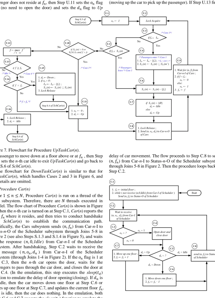
Performance analysis of ACSICD in Section III is evaluated and compared with previous proposed algorithms in this section. In Section IV.A, real data with time delays and the number of door openings have been recorded since 2017. We particularly analyze the collected data during the week of August 27, 2017. In Section IV.B, the simulated passenger requests of the scenario in [18] are treated as the input of ACSICD to produce the emulation results. Emulation with fixed and variable door open delays are used to evaluate the performance of ACSICD as well as the previous approaches.
A. Measurements of Door Open Delays
In [22], a sensor system is set up to monitor a six-floor elevator in the Department of Computer Science Building in National Chiao Tung University (NCTU). The sensor system has collected the data including the car status (idle/moving
up/moving down/door open/door close) and timestamps of door opening and closing since 2017. In this paper, the data collected during the week of August 27 in 2017 are used to investigate the door open delays 𝑡𝑑 and the delays 𝑡𝑓 of car moving up or down one floor. Table 2 lists the numbers of door openings and the expected value E[𝑡𝑑] in the week. The table indicates that the number of door openings in a week day is about 3 times of that in a weekend, and E[𝑡𝑑] ranges from 7.4 seconds to 8.27 seconds. Figure 9 illustrates the one-week histograms of the numbers of door openings occurring in 2-hour slots in a day.
From the curves, we observe one major peak at the 12~14 slot and two small peaks at the 8~10 and the 16~18 slots. Figure 10 plots E[𝑡𝑑]for every two-hour time slot in the week. The curves indicate that 𝑡𝑑 may vary significantly and using fixed 𝑡𝑑 to estimate the behavior of the elevator may not be practical (to be elaborated in Section IV.B). For car movement, we found that the delay 𝑡𝑓 is roughly fixed to 2 seconds.
Figure 9. The number of door openings in one week.
Figure 10. The expected door open delay E[𝑡𝑑] in one week.
Table 2. The collected elevator data in one week.
Date Number of door openings 𝐄[𝒕𝒅](seconds)
2017/8/27 (Sun) 468 8.15
2017/8/28 (Mon) 1147 8.18
2017/8/29 (Tue) 1162 7.69
2017/8/30 (Wed) 1018 8.27
2017/8/31 (Thr) 1149 7.64
2017/9/1 (Fri) 992 7.4
2017/9/2 (Sat) 334 7.72
B. Comparing ACSICD with the Previously Proposed Algorithms
In Appendices A and B, we have described several previously proposed algorithms. Emulation of the proposed ACSICD in Section III is conducted with the same scenario as the simulation experiment performed in Appendix A [18]. In our emulation experiments, the actual delays are emulated through the sleep() function. We measure the waiting time (when a passenger arrives at the start floor and when a car door opens), the travel time (when the passenger enters the car and when the car arrives at the target floor), and the journey time (the waiting time+the travel time).
Based on the 6-request scenario with fixed 𝑡𝑑 in [18], Table 3 lists the measured times for various algorithms. Among them, the duplex algorithm [23] is a conventional approach, which exercises full collective control of the cars. If the elevator system has completely served all incoming requests, then before the next request arrives, the idle cars are moved evenly among the floors. When the new requests arrive, the scheduler dispatches the cars to serve the nearest requests with the same moving direction. Details of other three genetic algorithms GA1, GA3 and GA4 are given in Appendix A.
The measured times for the Duplex, the GA1, the GA3 and the GA4 algorithms are obtained directly from the results reported in [9][18]. From Table 3, it is clear that our solution has improved the waiting times of the Duplex and the GA1 algorithms. Both GA3 and ACSICD have the same waiting time performance. GA4 has best waiting time performance, but has much longer travel time than ACSICD. Therefore, in terms of the journey time, ACSICD is better than GA4.
Table 3. Performance for various scheduling algorithms [18] with fixed 𝑡𝑑. Algorithm Waiting time (s) Travel time (s) Journey time (s)
Duplex 143 N/A N/A
GA1 143 N/A N/A
GA3 99 N/A N/A
GA4 80 205 285
ACSICD 99 163 262
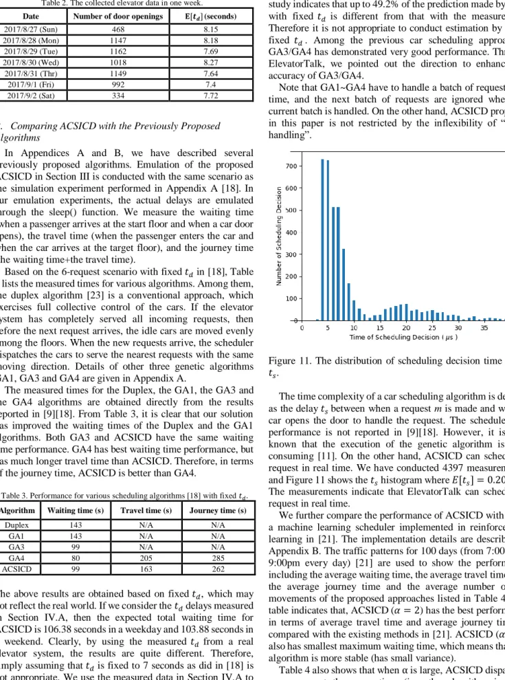
The above results are obtained based on fixed 𝑡𝑑, which may not reflect the real world. If we consider the 𝑡𝑑 delays measured in Section IV.A, then the expected total waiting time for ACSICD is 106.38 seconds in a weekday and 103.88 seconds in a weekend. Clearly, by using the measured 𝑡𝑑 from a real elevator system, the results are quite different. Therefore, simply assuming that 𝑡𝑑 is fixed to 7 seconds as did in [18] is not appropriate. We use the measured data in Section IV.A to conduct ACSICD to select the cars, and check if the selected cars are the same as GA3’s estimation by using fixed 𝑡𝑑. Our
study indicates that up to 49.2% of the prediction made by GA3 with fixed 𝑡𝑑 is different from that with the measured 𝑡𝑑. Therefore it is not appropriate to conduct estimation by using fixed 𝑡𝑑. Among the previous car scheduling approaches, GA3/GA4 has demonstrated very good performance. Through ElevatorTalk, we pointed out the direction to enhance the accuracy of GA3/GA4.
Note that GA1~GA4 have to handle a batch of requests at a time, and the next batch of requests are ignored when the current batch is handled. On the other hand, ACSICD proposed in this paper is not restricted by the inflexibility of “batch handling”.
Figure 11. The distribution of scheduling decision time delay 𝑡𝑠.
The time complexity of a car scheduling algorithm is defined as the delay 𝑡𝑠 between when a request m is made and when a car opens the door to handle the request. The schedule time performance is not reported in [9][18]. However, it is well known that the execution of the genetic algorithm is time consuming [11]. On the other hand, ACSICD can schedule a request in real time. We have conducted 4397 measurements, and Figure 11 shows the 𝑡𝑠 histogram where 𝐸[𝑡𝑠] = 0.201ms.
The measurements indicate that ElevatorTalk can schedule a request in real time.
We further compare the performance of ACSICD with RLS, a machine learning scheduler implemented in reinforcement learning in [21]. The implementation details are described in Appendix B. The traffic patterns for 100 days (from 7:00am to 9:00pm every day) [21] are used to show the performance including the average waiting time, the average travel time, and the average journey time and the average number of car movements of the proposed approaches listed in Table 4. The table indicates that, ACSICD (𝛼 = 2) has the best performance in terms of average travel time and average journey time as compared with the existing methods in [21]. ACSICD (𝛼 = 2) also has smallest maximum waiting time, which means that this algorithm is more stable (has small variance).
Table 4 also shows that when α is large, ACSICD dispatches more cars at the same time (i.e., the algorithm is more aggressive). In particular, when α = 2, ACSICD has the best
expected journey time performance of compared algorithms.
On the other hand, when α is small (α = 1 ), the required number of movement of the cars is less, which implies less energy consumption. The car movement number is an important output measure for energy consumption, but is not reported in the previous studies.
We use the same request traffic patterns in Table 4 to investigate the impact of α on ACSICD with 4 cars (i.e., 𝑁 = 4). Figure 12 plots the total waiting times and the total numbers of car movement per day for different α values. The figure indicates the intuitive results that as α increases, the waiting time decreases and the total number of car movement increases.
Specifically, by increasing α from 0.1 to 0.9, the waiting time is decreased by 38% at the cost of increasing the number of movement by 20%. Therefore, the operator can trade off the user experience (waiting) and energy consumption (car movement) by choosing an appropriate α value.
Table 4. Performance for various scheduling algorithms.
Algorithm
Max waiting time (s)
Average waiting time (s)
Average travel time (s)
Average journey time (s)
Average number
of moveme
nts per day ACSICD
(𝛼 = 1) 218 24.07 36.09 60.16 6504
ACSICD
(𝛼 = 2) 90 18.85 35.69 54.54 7325
LQF [21] 253 19.76 38.91 58.67 N/A
RLS [21] 218 17.42 40.65 58.07 N/A
Figure 12. Impact of 𝛼 (𝑁 = 4).
V. CONCLUSIONS
This paper proposed ElevatorTalk, an IoT based elevator scheduling system that allows the designer to develop a parallel car scheduling algorithm for an elevator system with multiple cars. We showed how to modularize the software for elevator components so that flexible and scalable car scheduling algorithms can be easily developed. ElevatorTalk consists of three subsystems: the Cars, the Elevator Car Operating Panel and the Scheduler subsystems. To create new car scheduling algorithms, the developer only needs to modify the Scheduler subsystem. The first two subsystems are standard, and can be reused for all elevator systems. These three subsystems work in parallel, and communicate with each other through sending and receiving messages. ElevatorTalk can connect to a real elevator
system to serve as the elevator management center. We proposed ACSICD in ElevatorTalk and compare it with previous proposed algorithms. Our study indicated that the ACSICD has better performance than the previous solutions.
Through this comparison, we pointed out where the previous approaches can be improved. We also show that the car scheduling decision can be quickly made in our approach within 0.201ms, and good performance in the time complexity is achieved. ElevatorTalk is used to analyze the behavior of commercial elevator systems for Yungtay Engineering Co.
[39].
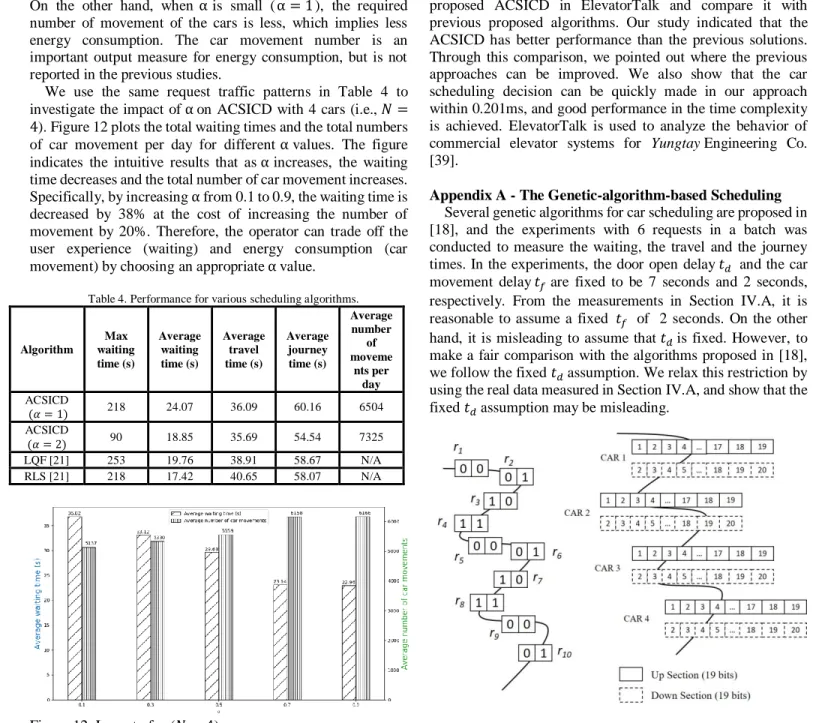
Appendix A - The Genetic-algorithm-based Scheduling Several genetic algorithms for car scheduling are proposed in [18], and the experiments with 6 requests in a batch was conducted to measure the waiting, the travel and the journey times. In the experiments, the door open delay 𝑡𝑑 and the car movement delay 𝑡𝑓 are fixed to be 7 seconds and 2 seconds, respectively. From the measurements in Section IV.A, it is reasonable to assume a fixed 𝑡𝑓 of 2 seconds. On the other hand, it is misleading to assume that 𝑡𝑑 is fixed. However, to make a fair comparison with the algorithms proposed in [18], we follow the fixed 𝑡𝑑 assumption. We relax this restriction by using the real data measured in Section IV.A, and show that the fixed 𝑡𝑑 assumption may be misleading.
(a) (b)
Figure A.1. The chromosome representations in (a) GA1 [9]
and (b) GA3 [18].
GA1 [9] and GA3 [18] are genetic-algorithm-based approaches, where GA3 is an enhancement of GA1. As in a traditional elevator system, both GA1 and GA3 as well as ACSICD assume that the target floors are determined after the passengers have entered the car. In genetic-algorithm based car scheduling, every request allocation assignment is represented by a chromosome encoded as a binary string. For example, Figure A.1(a) illustrates the chromosome of GA1. This chromosome is composed of 20 genes, where every gene is represented by one bit. For 1 ≤ 𝑖 ≤ 20, the i-th and the (i+1)-th bit (genes) are grouped to represent the elevator car that serves
the ⌊𝑖+12 ⌋-th request. Therefore, GA1 is designed for a 4-car system (every car is represented by 2 bits), and can handle at most 10 requests at a time. Denote a GA1 chromosome as a 20-bit string 𝑔1, where the car that serves the m-th request is represented by the (2𝑚 − 1)-th and (2𝑚)-th bits, which is denoted as 𝑔1(𝑚) . When the requests arrive, the GA1 algorithm is executed with the following steps.
Step GA1.1. Randomly generate 6 chromosomes with 10 requests.
Step GA1.2. Compute the fitness value of each chromosome according to the fitness function 𝐹(𝑔1) for every chromosome 𝑔1, which is the inverse of the total waiting time for serving the 10 requests based on the car scheduling encoded in 𝑔1, that is,
1
𝐹(𝑔1)= (1
10) ∑ 𝑇𝑚,𝑔1(𝑚)
10 𝑚=1
where 𝑇𝑚,𝑔1(𝑚) is the waiting time for car 𝑔1(𝑚) to serve the request 𝑟𝑚.; i.e., the delay between when the passenger mades the request and when the car arrives at the floor to pick the passenger. 𝑇𝑚,𝑔1(𝑚) for GA1 is similar to Eqs. (1)-(6) for GA3 to be elaborated later. Clearly, the larger the 𝐹(𝑔1) value, the better the waiting time performance.
Step GA1.3. Rank the 6 chromosomes according to their fitness values.
Step GA1.4. Replace the chromosome that has lowest fitness value with the one that has maximum fitness value.
Step GA1.5. Execute crossover process on chromosomes in pairs with a given probability.
Step GA1.6. Execute mutation process to randomly change the bit value of one gene in every chromosome.
Step GA1.7. Go to Step GA1.2 if the newly produced generation of chromosomes is not satisfied the converge condition. Otherwise, go to Step GA1.8.
Step GA1.8. Choose the chromosome with the best fitness value. Instruct the cars to serve the requests based on this chromosome.
Step GA1.9. Go to Step GA1.1. to handle next 10 requests.
GA3 extends the GA1 chromosome to 152 bits (Figure A.1 (b)) to deal with more requests (at most 2 × (𝐹 − 1)) within 4 cars where 𝐹 = 20. Since it is a four-car system, the 152-bit chromosome 𝑔3 is divided into four parts, one for each car. For 1 ≤ 𝑛 ≤ 4, the n-th part ranges from bit 38𝑛 − 37 to bit 38𝑛, which indicates the floors to be stopped by the n-th car.
Because the elevator system has 20 floors, the n-th part is further partitioned into two 19-bit sub-parts. The first sub-part (from bit 38𝑛 − 37 to bit 38𝑛 − 19) represents floors 1-19 and the value of a bit indicates if the car will stop at this floor when it moves up. On the other hand, the second sub-part (from bit 38𝑛 − 18 to bit 38𝑛) represents floors 2-20 and the value of a bit indicates if the car will stop at this floor when it moves down. The GA3 algorithm executes the following steps.
Step GA3.1. Generate 50 chromosomes randomly.
Step GA3.2. Compute the fitness value of each chromosome according to the fitness function (𝑔3) , which is the inverse of the total waiting for serving the M requests based on the car scheduling encoded in 𝑔3. This function is similar to (𝑔1) , and
the details are omitted.
Step GA3.3. Randomly select a pair of chromosomes (the parents).
Step GA3.4. The selected parent chromosomes produce a pair of offspring chromosomes (children) by crossover and mutation.
Step GA3.5. Replace the parent chromosomes with offspring chromosomes.
Step GA3.6. Go to Step GA3.2 if the number of generations is less than 100 (the converge criterion).
Step GA3.7. Choose the chromosome with the best fitness value. Instruct the cars to serve the requests based on this chromosome.
Step GA3.8. Go to Step GA3.1 to handle the next batch of requests.
To attain more precise waiting time estimation, GA3 uses an argument 𝑥𝑛 that denotes the number of known stops on the moving path of the n-th car from 𝑓𝑛 to 𝑓𝑠(𝑚) . Except for chromosome encoding and the definition of waiting time equations, GA1 and GA3 use similar processes to determine request assignment. Specifically, both GA1 and GA3 assume that the target floors of the requests are unknown during scheduling. We elaborate more on GA3 about the heuristics used in this algorithm.
If the n-th car is assigned to serve 𝑟𝑚, the waiting time 𝑇𝑚,𝑛 is defined as the sum of delays for moving the n-th car from 𝑓𝑛 to the start floor 𝑓𝑠(𝑚) of 𝑟𝑚 and the door open delays of the known stops within the movement path. In GA3, 𝑇𝑚,𝑛 is estimated by one of the following equations [18]. For 𝑑𝑛= 𝑈𝑝,
𝑇𝑚,𝑛
= {
[𝑓𝑠(𝑚) − 𝑓𝑛]𝑡𝑓+ 𝑥𝑛𝑡𝑑 ; 𝑓𝑠(𝑚) ≥ 𝑓𝑛 and 𝐷𝑚= 𝑈𝑝 (1) [2𝐹 − 𝑓𝑛− 𝑓𝑠(𝑚)]𝑡𝑓+ 𝑥𝑛𝑡𝑑 ; 𝐷𝑚= 𝐷𝑜𝑤𝑛 (2) [2𝐹 − 𝑓𝑛+ 𝑓𝑠(𝑚) − 2]𝑡𝑓+ 𝑥𝑛𝑡𝑑 ; 𝑓𝑠(𝑚) < 𝑓𝑛 and 𝐷𝑚= 𝑈𝑝 (3)
Symmetrical to Eqs (1)-(3), for 𝑑𝑛= 𝐷𝑜𝑤𝑛, we have
𝑇𝑚,𝑛
= {
[𝑓𝑛− 𝑓𝑠(𝑚)]𝑡𝑓+ 𝑥𝑛𝑡𝑑 ; 𝑓𝑠(𝑚) ≤ 𝑓𝑛 and 𝐷𝑚= 𝐷𝑜𝑤𝑛 (4) [𝑓𝑛+ 𝑓𝑠(𝑚) − 2]𝑡𝑓+ 𝑥𝑛𝑡𝑑 ; 𝐷𝑚= 𝑈𝑝 (5) [2𝐹 + 𝑓𝑛− 𝑓𝑠(𝑚) − 2]𝑡𝑓+ 𝑥𝑛𝑡𝑑 ; 𝑓𝑠(𝑚) > 𝑓𝑛 and 𝐷𝑚= 𝐷𝑜𝑤𝑛 (6)
Note that Eq. (1) estimates the waiting time for Case 1 in Figure 6, Eqs. (2) and (6) for Case 4, Eqs. (3) and (5) for Case 3 and Eq. (4) for Case 2. Through Eqs. (1)-(6), GA3 calculates the estimated waiting time of 𝑟𝑚 according to the chromosome at each iteration. Also note that computation for 𝑇𝑚,𝑛 of GA1 is similar to that for GA3 except that the factor 𝑥𝑛 is not considered. GA4 is the same as GA3, except that is used in a non-traditional elevator system where the target floors are determined before the passengers have entered the car.
Appendix B - Reinforcement-learning-based Scheduling Several scheduling algorithms are proposed in [21], including Dynamic Load Balancing, Collective, Longest Queue First (LQF), and AI methods based on reinforcement learning.
Among the three non-AI algorithms, LQF has the best performance, which always serves the request with the longest waiting time. The reinforcement learning scheduling algorithm (RLS) is implemented by extending LQF (Factor “𝑎" to be


![Table B.1. Factors for RLS [21].](https://thumb-ap.123doks.com/thumbv2/9libinfo/9660732.684066/11.918.87.833.92.1052/table-b-factors-for-rls.webp)
