PD Control of a Constrained Flexible Arm via Parallel Compensation

(1)

PD Control of a Constrained Flexible Arm via Parallel Compensation

Liang-Yih Liu ¹ , Hsiung-Cheng Lin ²

1 Department of Electrical Engineering, Chienkuo Technology University, Taiwan

2 Department of Electronic Engineering, National Chin-Yi University of Technology, Taiwan

1 [email protected], ² [email protected]

Abstract

In this paper, the force control of a constrained one-link flexible arm is investigated using a linear distributed parameter model, including internal damping of Kelvin-Voight type. To overcome the inherent limitations caused by the non-minimum phase nature of the noncollocation from the joint torque input and the tip contact force output, a new input induced by the root bending moment, and a contact force output generated by a parallel compensator are defined. The transfer function from the new input to the contact force output proves that it is not only strictly minimum phase but also a stable condition. A PD controller is then designed to improve the performance of the overall closed loop system. It is shown that asymptotic tracking of a desired contact force trajectory with internal stability can be achieved accurately. In order to obtain exact solutions of the infinite-dimensional system, the infinite product formulation is used throughout the paper. Numerical simulations are provided to verify the effectiveness of the proposed approach.

Keywords: constrained flexible arm, parallel compensator, minimum phase system, infinite- dimensional system.

Introduction

Force control of constrained flexible manipulators has received an increasing attention in recent years [1- 8]. Application of this research field include space robots used for satellite capturing and large space structure construction, and light weight industrial robots used for assembly, deburring and grinding tasks. The controller design for such force control problems is, however, quite difficult due to the distributed parameter nature of flexible arms and the noncollocation of torque actuation and contact force sensing.

Several methods have been proposed for force control of constrained flexible manipulators. Based on finite-dimensional approximate models, Chiou and Shahinpoor [1-2] studied a single-link and a two- link constrained flexible manipulators, and pointed out that the link flexibility is the main source of dynamic instability of the force controlled systems.

Later, in [3], Li indicated that an inherent limitation on the achievable bandwidth of force control occurs due to the presence of infinitely many non-minimum phase zeros. It is known that the flexible arm is inherently infinite-dimensional system in nature. As a result, the design of the finite-dimensional controller for the constrained one-link flexible arm may become more complicated using the distributed parameter model.

Obviously, this phenomenon posted a difficulty for such a model to be realized. Somehow, the problem was overcome using the Lyapunov method by Morita et al. [4] and Endo et al. [5]. The asymptotic stability of the closed-loop system was also achieved. But the proposed method may not guarantee the constrained one-link flexible manipulator system to be stable.

Recently, the passivity-based PD control using the infinite product formulation presented a satisfactory performance outcome in the linear distributed parameter model [6] However, the internal material damping was not considered in this study by Liu and Yuan [6. In the recent advanced progress, Bazaei and Moallem [7] proposed a distributed parameter model for a constrained flexible beam actuated at the hub, achieving the maximum control bandwidth. Bazaei and Moallem [8] extended their work to improve force control bandwidth of the constrained one-link arm through output redefinition. Unfortunately, the suppression of high frequency modes may pay a high cost because of degrading the performance attainable.

To overcome the limitations of above papers, this

paper is to develop the asymptotic tracking of a desired

contact force trajectory, being achieved using a

distributed parameter model of the constrained one-link

flexible arm. In order to reflect the intrinsic property of

internal friction of the link material, a distributed

parameter model which includes the widely used

Kelvin-Voight damping has been considered. To

remove the nonminimum phase obstacle relating the

joint torque input and the tip contact force output, a

new input induced by the root bending moment and its

derivative, and a virtual contact force output generated

by a parallel compensation are defined. It will prove

that the transfer function from the new input to the

virtual contact force output has all its infinite number of

poles and zeros lying in the open left-half plane. Then,

a PD control is used to improve the performance of the

(2)

infinite dimensional closed loop system. To preserve the exact poles and zeros of the system, the infinite product representations of transfer functions are employed throughout the paper. Numerical simulations are presented to demonstrate the excellent performance of the proposed approach.

Dynamic model

Derivation of Equations of Motion

The constrained one-link flexible arm depicted in Figure 1 is a uniform, homogeneous, Euler-Bernoulli beam of length  , mass per unit length  _{, and} flexural rigidity EI . The hub is modelled by a single- mass moment of inertia I where the driven torque h

)

 (t is applied. The end-effector has a concentrated mass m p , where the contact force exerted by the smooth rigid constraint surface is  (t ) _{. The} c _d  0 is a small damping constant of the beam material.The arm is assumed to move in a horizontal plane so that the gravity can be ignored. Let the X-axis be a fixed frame and x-axis be a floating frame, both coincident with the neutral axis of the beam.

The hub angular displacement  ^(t ⁾ is defined as the counterclockwise rotation of the x-axis with respect to the X-axis. Let ^v ⁽ ^x ^, ^t ⁾ be the small transverse deflection of the neutral axis of the beam with respect to the x-axis.



I

h

 ( ) t

 ( ) t v x t ( , )

m

_p

 ( ) t

X x

x u ( x ,t )

Figure 1. Schematic of a constrained flexible arm The equations of motion and the corresponding boundary conditions are (the details are rather involved and thus omitted)

      



 ( )

^

( ) ( , ) ( ) ( )

0

x x t v x t dx t t

t

I

_h

         

 ^ ^x    ⁽ ^t ⁾ ^ ^v   ⁽ ^x ^, ^t ⁾  ^ ^EI ^v x xx ⁽ ⁰ ^, ^t ⁾ ^ ^c d ^EI ^v  (1) x xx ⁽ ⁰ ^, ^t ⁾ ^ ⁰

 (2)

0 ) , 0

( t 

v (3)

0 ) , 0 ( t 

v _x ₍₄₎

0 ) , ( )

,

( t  c EI v t 

v

EI _x _x  _d  _x _x  (5)

) ( ) , ( )

,

( t c EI v t t

v

EI _x _xx   _d  _x _xx     (6)

Substitute Eqs. (2) and (6) into (1), and perform integration by parts with Eq. (5), an alternative form for Eq. (1) is obtained:

) ( ) , 0 ( )

, 0 ( )

( t EI v t c EI v t t

I _h     _x _x  _d  _x _x   (7) The root bending moment ^v x x ⁽ ⁰ ^, ^t ⁾ can be measured by a strain gauge sensor [4,8] and its derivative ^v  x x ⁽ ⁰ ^, ^t ⁾ can be detected by a full- bridge strain gauge [8]. This enables one to introduce a new joint input variable u (t ) _{such that}

) ( )

( t I t

u  _h  ^ ^ (8)

Non-Minimum phase transfer function from the input torque to the contact force

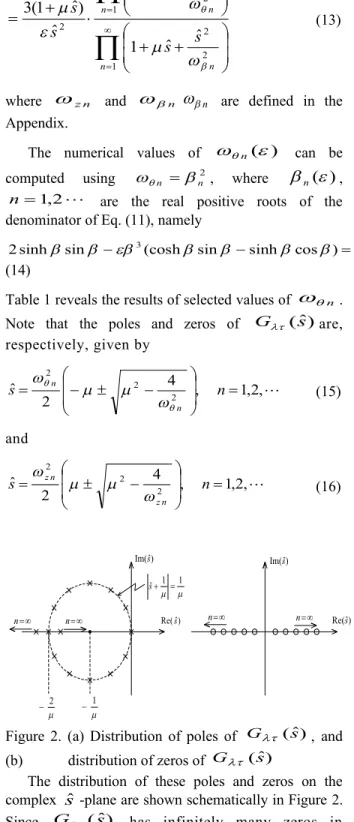
The transfer function can be derived by taking the Laplace transform of Eqs. (2)-(8) assuming zero initial conditions. Let s be the Laplace transform variable, and define the dimensionless parameters  , ,  ,  ^,

and sˆ as

c

d

EI

²

1

4

 



 

 

 

 , ₃

 

 I ^h

 _, _s

s EI

²

1 4

ˆ  



 

    (9)

 ^c ^s  ^s  ^s ^s 

EI _d 1 ˆ

ˆ 1

2 2 4 4



 

 

  ₍₁₀₎

With the application of infinite product representation of transcendental functions given in the Appendix, The results are (bearing in mind the implicit relation between s ^and  defined by Eq.(10)) as follows

) cos sinh sin

(cosh sin

sinh 2

sin sinh

ˆ ) (

ˆ ) : ( ˆ )

( ₃









 

  

 



 s 

s s G











 





 



  

 





 



  





1 2 2 1

2 2

ˆ ˆ 1

ˆ ˆ 1 1

n n

n z n

s s s s

 



 









 cos sinh cosh sin

sin sinh

1 ˆ )

( ˆ ) : ( ˆ )

( ₂



 



 u s 

s s G _u











 





 



  

 





 



  

 



1 2 2 1

2 2

2 ˆ

1 ˆ ˆ ˆ 1 ˆ

1 ˆ 3

n n

n z n

s s s s

s s

 



 



  ⁽¹²⁾

(3)









 

sin cosh sinh

cos

) cos sinh sin

(cosh sin

sinh 2 1 ˆ ) (

ˆ ) : ( ˆ ) (

3 3 



 



 u s s s

G _u











 





 



  

 





 



  

 



1 2

2 1

2 2

2 ˆ

1 ˆ ˆ ˆ 1 ˆ

ˆ ) 1 ( 3

n n

s s s s

s s





 



 (13)

where  z n _and  _ _n  _ _n are defined in the Appendix.

The numerical values of  _{ n} (  ) _{can be} computed using  _ n   n ² , where  _n ( ) ,

2  ,

 1

n are the real positive roots of the denominator of Eq. (11), namely

0 ) cos sinh sin

(cosh sin

sinh

2     ³      

(14)

Table 1 reveals the results of selected values of   n _.

Note that the poles and zeros of G _ _ (s ˆ ) are, respectively, given by

,  2 , 1 4 ,

ˆ 2 ² ₂

2  







 



   

 n

s

n n



 

 

(15)

and

,  2 , 1 4 ,

ˆ 2

2 2 2

 







 



  

 n

s

n z n

z

 

 

(16)



 1 ˆ  1  s

ˆ ) Re( s





n Re(s ˆ )

) ˆ Im(s



 1



 2





 n



n n  

) ˆ Im(s

Figure 2. (a) Distribution of poles of ^G   ^(s ^ˆ ⁾ , and (b) distribution of zeros of ^G   ^(s ^ˆ ⁾

The distribution of these poles and zeros on the complex sˆ -plane are shown schematically in Figure 2.

Since G _ _ (s ˆ ) has infinitely many zeros in 0

ˆ )

Re( s  , ^G   ^(s ^ˆ ⁾ is a nonminimum phase.

Similarly, G _ _u (s ˆ ) is also a nonminimum phase.

The effect of introducing the new input ^u ^(t ⁾ via root bending moment and its derivative is merely to change the poles of G _ _ (s ˆ ) to the poles of

ˆ ) (s

G _ _u .

Controller design

Removing the non-minimum phase obstacle by parallel compensation

Table 1 Values of roots of associated transcendental equations

(4)

To alleviate the non-minimum phase problem, the right half-plane zeros can be replaced by the left half- plane zeros by the method of redefinition of output.

Define a new virtual contact force ^f ^{( k} ^t ^, ⁾ such that    



 cos sinh cosh sin

) cos cosh 1 ( ) 1 ( ) sinh (sin

1 ˆ ) (

) ˆ , : ( ) ˆ , (

2 







 



k k

s u

k s k f

s G _f _u

 n   n ⁽ ^k ^ ⁰ ^. ⁷ ⁾ ^ ^ ⁿ

) 10 557 . 2

(    ^ ¹

 _ _n

1 ² ^. ⁸⁴⁷ ² 4 . 900 ² 816 2

. 1

2 4 . 082 ² 7 . 725 ² 992 2

. 3

3 8 . 145 ² ¹¹ ^. ⁰⁸⁶ ² 080 2

. 7

4 10 . 777 ² ¹⁴ ^. ⁰⁶⁶ ² 214 2

. 10

5 ₁₄ _. ₃₀₁ ² ¹⁷ ^. ³³⁶ ² 353 2

. 13

6 17 . 142 ² 20 . 371 ² 494 2

. 16

7 20 . 534 ² 23 . 604 ² 635 2

. 19

8 23 . 463 ² 26 . 666 ² 777 2

. 22

   _

odd n 

2 2 ) ( 1 3 ) 7 2 ( 1

 





 













 n n

2 2 ) ( 1 ) 1 2 ( 1

 





 









 n n

even n 

2 2 ) ( 1 3 ) 7 2 ( 1

 





 









 n n

2 2 ) ( 1 ) 1 2 ( 1

 





 













 n n

2

3 ) 3

4 ( 3

9108 . ) 3

4 ( 3

 





 













n

(5)

(17) where k is a real constant. It was shown in [9]

that for k  0 . 758 , one can write

 ^

  





 



 

 









1

2 ˆ 2

1 ˆ 1 1 2

) cos cosh 1 ( ) 1 ( ) sinh (sin

n n

s s

k k

 

 



(18) The numerical values can be computed using

2 n

n 

 _  , where  _n (k ) , n  1 , 2  are the real positive roots of the numerator of Eq. (18).

Selected values of   n are listed in Table 1. Thus, one has a minimum phase stable transfer function











 





 



  

 





 



  

 



1 2 2 1

2 2

2 ˆ

1 ˆ ˆ ˆ 1 ˆ

ˆ ) 1 ( ) 3

ˆ , (

n n

u

f s

s s s

s k s

s G





 



 

(19) where the distribution of poles and zeros of

) ˆ , ( k s

G _f _u takes similar pattern as shown in Figure 2(a). Note that the above redefinition of output is equivalent to the parallel compensation [10] as shown in Figure 3(a). It can be shown that the parallel compensator ^T ⁽ ^s ^ˆ ^, ^k ⁾ has the form



 cos sinh cosh sin

) sinh (sin

) cos cosh 1 ( ) 1 ) ( ˆ ,

( ₂







 

 

 k k s T











 





 



  

 





 



  

 



1 2 2 1

2 2

ˆ ˆ 1

ˆ ˆ 1 40

) 1 ( 11

n n

s s s s k





 

 

where  _ n   n ² and  _n (k ) , n  1 , 2  are the real positive roots of the equation

0 ) sinh (sin

) cos cosh 1

(        

 (21)

Selected values of   n are computed and listed in Table 1.

PD Control of the Parallel Compensated System For the control structure as shown in Figure 3(a), the objective is to make  ^(t ⁾ to track asymptotically a desired contact force trajectory  _d (t ) using an PD control, where k p and k are positive design _d constants, and k  0 . 758 . Obviously

ˆ ) ) ( ˆ , ( ˆ )

( 1

ˆ ) ) (

ˆ ,

( s

k s G s k k

s k k k

s

u _d

u f d

p

d

p 







 

(22) The characteristic equation of the closed-loop system is

0 ) ˆ , ( ˆ )

(

1  k _p  k _d s _  G _f _u s k  (23) To ensure that asymptotic tracking of output trajectories can be achieved even in the absence of internal damping. With G _f _u ( k s ˆ , ) given by setting

 0

 in Eq. (19), Eq. (23) becomes

ˆ 1 ˆ 1

1 ˆ ˆ )

( 3

1 2 2 2

1 2 2





 





 



 

 





 



 















n n

d

p s

s

s s

k k







(24)

Figure 3. (a) PD control of parallel compensated system; (b)overall closed-loop system in basic feedback loop

Clearly, the effect of P-control alone is merely to move all the closed-loop poles along the imaginary s ˆ -axis from s ˆ   j  _ , _n _ 1 _(set  _ ₀  0 ) to s ˆ   j  _ n , n  1 , 2 ,  as k p varies from 0 to  ^{. With} k p  k ^* p , Eq. (19) can be rewritten as









 





 



 

 





 



 

 







 N

s s s

k k

N

n n

N

n n

p

d 1 ,

1 ˆ 1 ˆ ˆ

1

1 2 2 1

2 2

*







(25)

It can be easily verified using a simple root locus plot that the D-control suffices to stabilize the closed- loop system for all ⁰ ^ k ^* p ^ ^ and 0  k _d   . Therefore, it is reasonable to conjecture that the

(a)

(b)

(6)

damping effect should be enhanced when internal damping are considered. Let the roots of Eq. (23) be written as

 1 , 1 , 2 , 

ˆ  ⁴ s    j  ² n 

s _n  EI _n  _n  _n  _n  _n

(26) where  _n (  _n   _n _ ₁ ) _and  _n are the natural frequency and damping ratio of the n-th closed-loop pole. Using Eq. (19), one may write Eq. (23) as



    





 



  

 







 



  



N

n n

N

n n

d p

s s s s

s s

s k k

1 2 2 2

1

2 2 ˆ

1 ˆ ˆ ˆ

1 ˆ ˆ ) 1 ˆ )(

( 3



  

 





 







 



  

  ^



s N k s

N

n n n n

p ˆ ˆ ,

2 1 3

1

1 2 2

 

 ₍₂₇₎

Using Eq. (22) for ^u ⁽ ^s ^ˆ ^, ^k ⁾ and G _ _u (s ˆ ) , ˆ )

(s

G _ _u given by Eqs. (19) and (12)-(13), the closed-loop responses of some relevant variables can be computed as follow.





 





 



  

 





 



  



 







 



 

 







 s N

s s

s s s

k s

s k _N _d

n n n

n N

n z n

p

d ( ˆ ),

ˆ 2 ˆ

1 ˆ ˆ 1 ˆ ) 1 ( 1 ˆ

ˆ )

( ₁

1 2 2 1

2 2



 



 





(28)





 





 



  

 





 



  



 







 



 

 







 s N

s s

s s s

k s

s k _N _d

n n n

n N

n n

p

d ( ˆ ),

ˆ 2 ˆ

1 ˆ ˆ 1 ˆ )

1 ( 1 ˆ

ˆ )

( ₁

1 2 2 1

2 2





 

 



 ^



(29) Note that the above results are exact closed-loop solutions of the infinite-dimensional force control system. To perform the inverse Laplace transform,

sˆ can be replaced by s EI

 4

 . The closed-loop

time responses can be computed within an arbitrary degree of accuracy by taking N as large as required. In order to find the exact values (to the extent of numerical accuracy) of the closed-loop poles (i.e. the roots of Eq. (23), G _f _u ( s ˆ , k ) given by Eq.

(17) must be used. Using either of

4 1 2

1 ˆ ˆ 2

1  





 







 

s s j

  , the equation

sin 0 cosh sinh

cos

) cos cosh 1 ( ) 1 ( ) sinh ) (sin

( ˆ

1 ₂ 









 

 



k s k

k

k _p _d

(30)

can be solved numerically to yield  n _and  _n , 2 

,

 1

n . The control structure of Figure. 3(a) can be converted to the basic feedback loop as shown in Figure. 3(b). Using Eqs. (13) and (20), it is not difficult to show that the transfer function of the compensator is

)]

sin (sinh

) cos cosh 1 )[(

1 ˆ )(

(

)]

cos sinh sin

(cosh

) sin cosh cos

(sinh

sin sinh 2

[ ˆ ) ) (

( ˆ

1 2























 



k s k k

s k s k

C

d p

d

p 

(31)

Numerical simulation

The effectiveness of the proposed control approach is evaluated here through numerical simulation using the parameters of an experimental apparatus described in [11]. These parameters are: ^ ^ ⁰ ^. ¹¹⁴ ^kg ^/ ^m ,

2 . 23

EI  _N  _m ² ,   0 . 7 ^m,and ^I ^h ^ ⁰ ^. ⁰¹

m

2

kg  (   2 . 557  10 ^ ¹ ), c _d  1 . 17  10 ^ ⁴

s (   3 . 406  10 ^ ³ ).

The values of   n _,  _z _n _,  _ _n _,  _ _n _and

 n

 can be found in the Appendix and Table 1. The virtual contact force parameter and controller gain that resulted in good performance were selected as

7 .

 0

k , k p ^ ² ^. ⁹⁷⁵ and k _d  1 . 826 . The desired contact force trajectory was selected as

) 60 61

1 ( 5 )

( ⁵³ ^t ⁵⁴ ^t

d t   e ^  e ^

 (32)

which results in lim ( )  lim ( , 0 . 7 )  5







 t f t

t

t  _N,

10 2

52 . 3 ) (

lim ^



 t  

t  _rad,

15 . 0 ) , 0 (

lim 



 v _xx t

t m ^ ¹ , and lim ( )  3 . 5



 t

t 

N-m. The simulation results which are hardly discernible for N  M  4 are shown in Figure 4. The responses due to the disturbance   ^:   ⁽ ⁰ ⁾

2 2 2 10

10 52 .

3  ^    ^

 rad perturbed from the

steady state solution can be computed using Figure 3(b)

and are shown in Figure 5.

(7)

Conclusions

In this paper, the contact force control of a constrained one-link flexible arm has been investigated based on a linear distributed parameter model including internal damping of Kelvin-Voight type. With the joint torque as the input and the tip contact force as the output, the noncollocated system is non-minimum phase. Using the feedback of root bending moment and its derivative to generate a new input and the redefinition of output via parallel compensation, a minimum phase stable transfer function is obtained for noncollocated system. For the new transfer function, it has been shown that perfect asymptotic tracking of a desired contact force trajectory with internal stability can be achieved using a PD controller. Unlike most traditional approaches based on truncated models,

which will generally suffer from control and observation spillover problems, exact solutions have been obtained in this paper for the noncollocated infinite-dimensional force control system. Numerical simulations have been presented to verify the excellent performance of the proposed approach. The advantages of using infinite product formulation throughout the paper have also been emphasized.

References

[1] C hiou, B.C., and Shahinpoor, M., 1988, “Dynamic Stability Analysis of a One-Link Force -Controlled Flexible Manipulator,” Journal of Robotic Systems, Vol. 5, No. 5, pp. 443-451.

[2] Chiou, B.C., and Shahinpoor, M., 1990, “Dynamic Stability Analysis of a Two-Link Force- Controlled Flexible Manipulator,” ASME Journal of Dynamic Systems, Measurement, and Control, Vol.

112, No. 6, pp. 661-666.

[3] Li, D., 1990, “Tip-Contact Force Control of One-Link Flexible Manipulator: An Inherent Performance Limitation,” Proceedings of 1990 American Control Conference, San Diego, CA., pp. 697-701.

[4] Morita, Y., Matsuno, F., Ikeda, M., Ukai, H., and Kando, H., 2002, “Experimental study on PDS force control of a flexible arm considering bending and torsional deformation,” 7 ^th International Workshop on Advanced Motion Control, Maribor, Slovenia, pp.

408-413.

[5] Endo, T., and Matsuno, F., 2004, “Dynamics based force control of one-link flexible arm,” SICE 2004 Annual Conference, Sapporo, Vol. 3, pp. 2736-2741.

[6] Liu, L. Y., and Yuan, K., 2003, “Noncollocated Pasivity-Based PD Control of a Single-Link Flexible Manipulator,” Robotica, Vol. 21, No. 2, pp. 117-135.

[7] Bazaei, A., and Moallem, M., 2009, “Force Transmission Through a Structurally Flexible Beam:

Dynamic Modeling and Feedback Control,” IEEE Transactions On Control Systems Technology, Vol.

17, No. 6, pp. 1245-1256.

[8] Bazaei, A., and Moallem, M., 2010, “Improving Force Control Bandwidth of Flexible- Link Arms Through Output Redefinition,” IEEE/ASME Transactions On Mechatronics, Vol. 15, No. 5, pp. 1- 7.

[9] Yuan, K., and Liu, L.Y., 2000, “Achieving Mini-mum Phase Transfer Function for a Noncollocated Single- Link Flexible Manipulator,” Asian Journal of Control, Vol. 2 , No. 3, pp. 179-191.

[10] Geniele, H., Potel, R. V., and Khorasani, K., 1997,

“End-Point Control of a Flexible-Link Manipulator : Theory and Experiments,” IEEE Transactions On Control Systems Technology, Vol. 5, No. 6, pp. 556- 570.

[11] Matsuno, F., Umeyama, S., and Kasai, S., 1997,

“Experimental Study on Robust Force Control of a Flexible Arm with a Symmetric Rigid Tip Body,”

Proceedings of 1997 IEEE International Conference

0

⁰

0.1 0.2 0.3

1 2 3 4 5 5.5

0

⁰

0.1 0.2 0.3

1 2 3 4

D es ir ed a nd c on ta ct f or ce s, N C on tr ol to rq ue , N -m

0 0.1 0.2 0.3

-30

- 25

-

20 -

15 - 10

- 5

0 5

0 0.1 0.2 0.3

- 0.5

-0.3 -0.1 0 0.1 0.3

3

0.5

10

^



C on ta ct f or ce s, N

Figure 4. (a)  ^(t ⁾ ,  _d (t ) ; (b)  ^(t ⁾

Figure 5. (a)  ^(t ⁾ ; (b)  ^(t ⁾

time, s (b) time, s

(a)

time, s (a)

time, s (b)

C on tr ol to rq ue , N -m

(8)

on Robotics and Automation, Albuquerque, New Mexico, pp. 3136-3141.

Appendix

The infinite product expansions for transcendental functions used in this paper are summarized as follows [6,9]. In accordance with the context of this paper,

2 4

1 ˆ

ˆ 

 ^ ^

 s

s is used whenever it is appropriate.

A1.  ^

  











 

 





1 2

ˆ 2

1 ˆ 1 1 2

sinh sin

n z n

s s 

 



2 _n 2 n

z  a

 , tanh a _n  tan a _n  0 ,

0 ( a _n  real )

 4 ) (  1

 n

a _n as ⁿ ^ ^

1  2 ( 2 . 365 ) 2

 z ,  _z ₂  2 ( 5 . 498 ) ² ,

3  2 ( 8 . 639 ) 2

 z ,  _z ₄  2 ( 11 . 781 ) ² ,

5  2 ( 14 . 923 ) 2

 z ,  _z ₆  2 ( 18 . 064 ) ²

A2.  ^

  





 



 

 



1 4 4

2 ˆ 2

1 ˆ 1 1 sinh

sin

n n

s

s 

 



A3.

 ^

  





 



 

 





1

2 3 ˆ 2

1 ˆ 1 1 3

sinh 2 cos sin

cosh

n n

s s  _

 



n 2 n  c

  , tanh c _n  tan c  0 ( c _n  0 , )

real

 4 ) (  1

 n

c _n as ⁿ ^ ^

1  3 . 927 2

  ,  _ 2  7 . 069 ² ,

3  10 . 210 2

  ,

4  13 . 352 2

  ,  _ 5  16 . 493 ² ,

6  19 . 635 2

 

A4.  ^

  





 



 

 





1 2

p

ˆ 2

1 ˆ 1 1 2 cos cosh 1

n n

s s 

 



p n  b 2 n

 , cosh b _n cos b _n  1  0 ( b _n  0 , )

real

 2 ) (  1

 n

b _n as ⁿ ^ ^

1  1 . 875 2

 p ,  _p 2  4 . 694 ² ,

3  7 . 855 2

 p ,

4  10 . 996 2

 p ,  _p 5  14 . 137 ² ,

6  17 . 279 2

 p

Note that the asymptotic expressions are quite accurate

(to three decimal places) for n  5 .

PD Control of a Constrained Flexible Arm via Parallel Compensation