關於231-有禁排列統計量多項式遞迴關係之研究

全文

(1)國立屏東大學應用數學系碩士班碩士論文 Department of Applied Mathematics National Pingtung University Master’s Thesis. 關於 231-有禁排列統計量多項式遞迴關係之研究 On a Study of Recurrence Relations of Some Statistic-Polynomials on 231-avoiding Permutations. 指導教授：傅東山博士 Advisor: Dr. Tung-Shan Fu 研究生：許青之 Student: Ching-Chih Hsu. 中. 華. 民. 國. 108 年. June 2019. 6 月.

(2)

(3) 摘要我們考慮 231-有禁排列以主指標及下降數雙統計量的 Euler-Mahonian 多項式，並模仿 Dokos, Dwyer, Johnson, Sagan, Selsor 的方法證明這個多項式的遞迴關係。我們另外考慮 231-有禁排列以逆序數及右至左極小元素雙統計量的 Mahonian-Stirling 多項式，並且使用了 Dyck 路徑和二元樹二種方法證明了這個多項式的遞迴關係。最後，我們也討論了關於 Stump 所建立 231-有禁排列與 Dyck 路徑雙射對應關係以及 Petersen 的描述，和上述統計量的關聯。. 關鍵字：231-有禁排列、Dyck 路徑、二元樹. i.

(4) Abstract We consider the bivariate polynomials of the 231-avoiding permutations with respect to major index and descent number, and make use a method of Dokos, Dwyer, johnson, Sagan, Selsor to prove a recurrence relation for the polynomials. We also consider the polynomials of the 231-avoiding permutations with respect to inversion number and the number of right-to-left minima. Then we use two methods to prove a recurrence relation for the polynomials in terms of Dyck paths and binary trees, respectively. Finally, we discuss a bijection between 231-avoiding permutations and Dyck path established by Stump, and Petersen’s description and the connection of the statistics mentioned above.. Keyword: 231-avoiding permutation, Dyck path, binary tree. ii.

(5) 目錄中文摘要 . . . . . . . . . . . . . . . . . . . . . . . . . . . . . . . . . . . . . . . . . . . . i 英文摘要 . . . . . . . . . . . . . . . . . . . . . . . . . . . . . . . . . . . . . . . . . . . . ii 目錄 . . . . . . . . . . . . . . . . . . . . . . . . . . . . . . . . . . . . . . . . . . . . . . . iii 圖形目錄 . . . . . . . . . . . . . . . . . . . . . . . . . . . . . . . . . . . . . . . . . . . . iv 表格目錄 . . . . . . . . . . . . . . . . . . . . . . . . . . . . . . . . . . . . . . . . . . . . v 1 緒論 . . . . . . . . . . . . . . . . . . . . . . . . . . . . . . . . . . . . . . . . . . . . . 1 1.1 研究背景 . . . . . . . . . . . . . . . . . . . . . . . . . . . . . . . . . . . . . . . 1 1.2 研究目的 . . . . . . . . . . . . . . . . . . . . . . . . . . . . . . . . . . . . . . . 2 1.3 研究工具 . . . . . . . . . . . . . . . . . . . . . . . . . . . . . . . . . . . . . . . 5 2 在 231-有禁排列中主指標及下降數的雙統計量多項式 . . . . . . . . . . . . . 7 2.1 排列膨脹 . . . . . . . . . . . . . . . . . . . . . . . . . . . . . . . . . . . . . . . 7 2.2 定理 1.1 的證明 . . . . . . . . . . . . . . . . . . . . . . . . . . . . . . . . . . . 8 2.3 用 Maxima 程式進行驗證 . . . . . . . . . . . . . . . . . . . . . . . . . . . 10 3 在 231-有禁排列中逆序數及右至左極大元數的雙統計量多項式. ..... .. 11. . . . . .. . . . . .. 11 12 13 14 17. 4 Dyck 路徑和 231-有禁排列 . . . . . . . . . . . . . . . . . . . . . . . . . . . . .. 18. 4.1 Stump 的雙射對應 . . . . . . . . . . . . . . . . . . . . . . . . . . . . . . . . 4.2 將 231-有禁排列的下降段對應到 Dyck 路徑 . . . . . . . . . . . . . . . . 4.3 其他的一些性質 . . . . . . . . . . . . . . . . . . . . . . . . . . . . . . . . . .. 18 19 20. 5 未來研究方向 . . . . . . . . . . . . . . . . . . . . . . . . . . . . . . . . . . . . . .. 21. 參考文獻 . . . . . . . . . . . . . . . . . . . . . . . . . . . . . . . . . . . . . . . . . . .. 22. 附錄 . . . . . . . . . . . . . . . . . . . . . . . . . . . . . . . . . . . . . . . . . . . . . .. 23. 3.1 3.2 3.3 3.4 3.5. Catalan 數和 Dyck 路徑堆疊排序和 Dyck 路徑 . 定理 1.2 的第一種證明 . 定理 1.2 的第二種證明 . 用 Maxima 程式進行驗證. . . . .. . . . . .. . . . . .. . . . . .. . . . . .. . . . . .. 3 iii. . . . . .. . . . . .. . . . . .. . . . . .. . . . . .. . . . . .. . . . . .. . . . . .. . . . . .. . . . . .. . . . . .. . . . . .. . . . . .. . . . . .. . . . . .. . . . . .. . . . . .. . . . . .. . . . . .. . . . . ..

(6) 圖形目錄圖 2.1. π = 231 和 231[σ1, σ2, σ3] 圖 2.2. σ ∈ Avn(231). .... ..... ...... ..... ..... ..... .. 7. . ..... ..... ..... ...... ..... ..... ..... .. 9. 圖 3.1. s(32154) = 12345. . . . . . . . . . . . . . . . . . . . . . . . . . . . . . . . . . . . . . 12. 圖 3.2. Dyck 路徑的山峰和面積. . . . . . . . . . . . . . . . . . . . . . . . . . . . . . . . . . 13. 圖 3.3. 一個二元樹與 231-有禁排列. . . . . . . . . . . . . . . . . . . . . . . . . . . . . . . . 15. 圖 4.1. 將長度為 6 的 Dyck 路徑對應到簡單的轉置. . . . . . . . . . . . . . . . . . . . . . . 18. 圖 4.2. 由 231-有禁排列的下降段建構的 Dyck 路徑. . . . . . . . . . . . . . . . . . . . . . . 19. 圖 4.3. 將 Dyck 路徑以直線 y = x 鏡射圖 4.4. 雙升統計量. . . . . . . . . . . . . . . . . . . . . . . . . . . . . . 20. . . . . . . . . . . . . . . . . . . . . . . . . . . . . . . . . . . . . . . . . 20. 4 iv.

(7) 表格目錄表 3.1. 長度為 4 的 231-有禁排列分別對 inv(σ) 和 rlmin(σ) 的分佈表 3.2. 二元樹的細分. . . . . . . . . . . . . . 15. . . . . . . . . . . . . . . . . . . . . . . . . . . . . . . . . . . . . . . 15. v5.

(8) 1 緒論 1.1 研究背景設 Sn 是所有長度為 n 的排列所成的集合，一長度為 n 的排列 (permutation) σ 是指從 {1, 2, ..., n} 到 {1, 2, ..., n} 的雙射 (bijection)。令 σ = σ1...σn ∈ Sn, 其中 σi =σ(i), 1 ! i ! n。考慮排列統計量當 i < j 且 σi > σ j 時，我們稱數對 (σi , σ j ) 為 σ 的. 逆序 (inversion), 以符號 inv(σ) 表示 σ 的逆序數，即 inv(σ) = #{(σi , σ j ): i < j , σi >σ j }。若以圖形表示排列，例如 σ = 314265 可以表示成下圖：. 則 inv(σ) 為連線的交點數量，此例中 inv(σ) = 4。因為對任意長度為 n 的排列 σ, ∀i ∈ {1, 2, ..., n}, 序列 i, σ(i), σ 2(i), σ 3(i), ... 不可能全部不同，若 k 為最小的數，使得 σ k(i) = i, 則 (i, σ(i), σ 2(i), ..., σ k−1(i)) 形成一個輪換 (cycles), 這個輪換的長度即為 k , 因此也記做 k -輪換。特別的稱長度為 1 的輪換就是 σ 的固定點 (fixed point), 長度為 2 的輪換則稱做轉置 (transposition)。 σ 也可以用這種輪換分解(cycle decomposition)來表示，例如：σ = 23145 = (123) (4)(5)。在 Sn 中我們可以討論許多有趣的統計量，以及排列按這些統計量對應的生成函數，例如 Rodriguez 早在 1837 年就提出 Sn 中排列按逆序數統計量的分布方式如下： !. q inv(σ) = (1 + q)(1 + q + q 2)...(1 + q + ... + q n−1).. σ∈Sn. σ 的下降 (descents) 指的是 σ 中的位置 i, 滿足 σi > σi+1 其中 1 ! i ! n − 1。 " 設 Des(σ) 是這種位置的集合。定義統計量 maj(σ) = i 並稱為排列的主指標 i∈Des(σ) " maj(σ) " inv(σ) (major index), 由 Percy MacMahon 所提出，並且證明了 q = q . σ∈Sn. σ∈Sn. 我們以簡單的 n = 4 為例，可以將 S4 中的 24 個元素以 maj(σ) 或 inv(σ) 分類，得到的生成函數都是 1 + 3q + 5q 2 + 6q 3 + 5q 4 + 3q 5 + q 6, 通常稱與逆序數相同分佈的統計量為 Mahonian 統計量。 1.

(9) 統計量 des(σ) 則是 Des(σ) 的元素數量，屬於 Eulerian 數, 是數學家 Euler 在研究交錯的 ζ 函數時所得到的[8]。為了方便我們之後的說明，在此另外定義四個統計量： 1. 稱 σk 為 σ 的左至右極大元素 (left-to-right maximum), 當 1 ! j < k 時 σ j < σk 。用 lrmax(σ) 表示 σ 中這種元素的數量。 2. 稱 σk 為 σ 的左至右極小元素 (left-to-right minimum), 當 1 ! j < k 時 σ j > σk 。用 lrmin(σ) 表示 σ 中這種元素的數量。 3. 稱 σk 為 σ 的右至左極大元素 (right-to-left maximum), 當 k < j ! n 時 σj < σk 。用 rlmax(σ) 表示 σ 中這種元素的數量。 4. 稱 σk 為 σ 的右至左極小元素 (right-to-left minimum), 當 k < j ! n 時 σk < σ j 。用 rlmin(σ) 表示 σ 中這種元素的數量。這幾個統計量和 σ 輪換的數量有相同的分佈： !. tcyc(σ) = t(t + 1)(t + 2)...(t + n − 1). σ∈Sn. 符號 cyc(σ) 表示 σ 的輪換數量，其係數被歸類為無正負號的第一類 Stirling 數 [16]。我們也可以給定二個統計量來探討它的分佈情形，例如 (des(σ), maj(σ)) 是 “ Euler-Mahonian” 統計量序對，有如下分佈[10]: ". tdes(σ) q maj(σ). σ∈Sn n #. i=0. = (1 − tq i). !. tr(1 + q + ... + q r)n.. r!0. 若二統計量 st1, st2 有如下分佈則稱為 “Mahonian-Stirling” 統計量序對[12]: !. q st1(σ)tst2(σ) = t(t + q)(t + q + q 2)...(t + q + ... + q n−1).. σ∈Sn. 1.2 研究目的設 k ! n, σ 中的元素 σi1, ..., σik 稱為 σ 長度為 k 的子序列，其中 i1 < ... < ik。令 σ ∈ Sn, τ ∈ Sk, 我們稱 σ 為 τ -有禁排列 (τ -avoiding permutation), 是指 σ 不存在長度為 k 的子序列與 τ 有相同的大小順序關係。因此對於 τ ∈ S3, 我們有下列六種 2.

(10) 有禁排列： •. 123-有禁排列為 σ 不包含子序列 σi , σ j , σk 使得 σi < σ j < σk,. •. 132-有禁排列為 σ 不包含子序列 σi , σ j , σk 使得 σi < σk < σ j ,. •. 213-有禁排列為 σ 不包含子序列 σi , σ j , σk 使得 σ j < σi < σk,. •. 231-有禁排列為 σ 不包含子序列 σi , σ j , σk 使得 σk < σi < σ j ,. •. 312-有禁排列為 σ 不包含子序列 σi , σ j , σk 使得 σ j < σk < σi,. •. 321-有禁排列為 σ 不包含子序列 σi , σ j , σk 使得 σk < σ j < σi. 用符號 Avn(τ ) 表示 Sn 中所有 τ -有禁排列所成的集合。對於 τ ∈ S3, 這六種 1. 集合的元素個數 #Avn(τ ), 都是 Catalan 數 cn = n + 1. !. 2n n. ". [14]。Stanley 列舉了許. 多關於 Catalan 數的組合解釋 [16], 我們之後會用到這些 Catalan 數的組合工具幫助我們證明與推論。 Dokos 等學者在研究排列的模式和統計量時，藉由排列膨脹 (inflations of permutations) 的手法，得到了以下結果[6]: 定理. (Dokos, Dwyer, Johnson, Sagan, Selsor [6]) 令 !. In(q) =. q inv(σ). σ∈Avn(312). 為 312-有禁排列以逆序數的統計量生成函數，並且令其初始值 I0(q) = 1, 對所有 n ≥ 1 而言有下列遞迴關係：. In(q) =. n−1 ! k=0. 並且若令. (1.1). q kIk(q)In−k −1(q). Cn(q) =. !. q inv(σ). σ∈Avn(132) !. ˜ (q) = q 是 Carlitz 所定義的 q-Catalan 數[ 7], 且 C Cn(q) =. !. q inv(σ) =. σ∈Avn(132). Cñ(q) =. !. n 2. ". Cn(q −1), 則對 n " 0, 會得到：. !. q inv(σ). σ∈Avn(213). q inv(σ) =. σ∈Avn(231). !. σ∈Avn(312). 3. q inv(σ).

(11) 但是相同手法卻無法使用在 321-有禁排列的情形。直到 Cheng, Elizalde, Kasraoui, Sagan 在 [4] 中得到 321-有禁排列以逆序數和左至右極大元素的 Mahonian-Stirling 雙統計量生成函數： !. In(q, t) =. q inv(σ)tlrmax(σ). σ∈Avn(321). In(q, t) 有如下遞迴關係： In(q, t) = tIn−1(q, t) +. n−2 ! k=0. q k+1Ik(q, t)In−k −1(q, t). (1.2). 我們的研究目的有三： (A) 考慮 231-有禁排列以主指標及下降數雙統計量的 Euler-Mahonian 多項式，定義 Mn(q, t) =. !. q maj(σ)tdes(σ). σ∈Avn(231). 令其初始值 M0(q, t) 及 M1(q, t) 都是 1, 前五項的結果： M1(q, t) M2(q, t) M3(q, t) M4(q, t) M5(q, t). = = = = =. 1 1 + qt 1 + (2q + q 2)t + q 3t2 1 + (3q + 2q 2 + q 3)t + (3q 3 + 2q 4 + q 5)t2 + q 6t3 1 + (4q + 3q 2 + 2q 3 + q 4)t + (6q 3 + 5q 4 + 6q 5 + 2q 6 + q 7)t2 +(4q 6 + 3q 7 + 2q 8 + q 9)t3 + q 10t4. 我們證明下列定理：定理 1.1. 令 Mn(q, t) =. ". q maj(σ)tdes(σ) , 且 M0(q, t) = M1(q, t) = 1 為初始值，則. σ∈Avn(231). Mn(q, t) 有以下遞迴關係：. Mn(q, t) = qt · Mn−1(q, qt) + Mn−1(q, t) +. n−2 ! k=1. q k+1tMk(q, t)Mn−k −1(q, q k+1t). (B) 另外考慮 231-有禁排列中以逆序數和右至左極小元素的 Mahonian-Stirling 雙統計量生成函數雙統計量多項式，定義 Cn(q, t) =. !. q inv(σ)trlmin(σ). σ∈Avn(231). 4.

(12) 其前 5 項的結果如下： C1(q, t) C2(q, t) C3(q, t) C4(q, t) C5(q, t). = = = = =. t qt + t2 q 3t + (2q + q 2)t2 + t3 q 6t + (q 2 + 2q 3 + 2q 4 + q 5)t2 + (3q + 2q 2 + q 3)t3 + t4 q 10t + (2q 4 + 3q 6 + 2q 7 + 2q 8 + q 9)t2 + (3q 2 + 5q 3 + 4q 4 + 5q 5 + 2q 6 + q 7)t3 +(4q + 3q 2 + 2q 3 + q 4)t4 + t5. 在第 3 章我們證明下列遞迴式，並提出二種不同的組合證明。定理 1.2. 令 Cn(q, t) =. ". q inv(σ)trlmin(σ) , 初始值 C0(q, t) = 1, 則 Cn(q, t). σ∈Avn(231). 會滿足下列遞迴關係：. Cn(q, t) = tCn−1(q, t) +. n−1 !. q kCk(q, t)Cn−k−1(q, t). k=1. (C) 最後在第 4 章中，我們介紹更多不同的雙射關係連結本文的 231-有禁排列與 Dyck 路徑，從這些不同的雙射對應，導出 231-有禁排列中下降數和右至左極小元素二個統計量的分佈，以及其在 Dyck 路徑中代表的意義。. 1.3 研究工具這篇論文中會使用到 Maxima 幫助我們進行驗證，我們把程式碼放在 lib.txt 文件檔中，如附錄所示，每次使用前需要先載入檔案 lib.txt，我們利用 Maxima 將所有長度為 n 的排列找出來後，逐一檢測每個元素的統計量，將得出的生成函數與我們的遞迴式相比較。例如，我們要驗證 S4 的 inv(σ) 和 maj(σ) 等分佈， " maj(σ) " inv(σ) 可以這樣做：令 MQ(n) = q , IQ(n) = q ，相關程式碼參考附錄 σ∈Sn. σ∈Sn. ，Maxima 程式計算如下：. (%i1) batchload("/Users/change/lib.txt")$ (%i2) powerdisp:true$ (%i3) IQ(4); (%o3) 1 + 3 q + 5 q 2 + 6 q 3 + 5 q 4 + 3 q 5 + q 6 (%i4) MQ(4); (%o4) 1 + 3 q + 5 q 2 + 6 q 3 + 5 q 4 + 3 q 5 + q 6 5.

(13) 底下是我們驗證 (1.1) 式的方法，其中 CQ_hat(n) = Cñ(q) = In(q)： (%i5) CQ_hat(0); (%o5) 1 (%i6) CQ_hat(1); (%o6) 1 (%i7) CQ_hat(2); (%o7) 1 + q (%i8) CQ_hat(3); (%o8) 1 + 2 q + q 2 + q 3 (%i9) CQ_hat(4); (%o9) 1 + 3 q + 3 q 2 + 3 q 3 + 2 q 4 + q 5 + q 6 (%i10) CQ_hat(5); (%o10) 1 + 4 q + 6 q 2 + 7 q 3 + 7 q 4 + 5 q 5 + 5 q 6 + 3 q 7 + 2 q 8 + q 9 + q 10 (%i11) CQ_hat(6)-expand(sum((q^k)*CQ_hat(k)*CQ_hat(5-k),k,0,5)); (%o11) 0. 6.

(14) 2 在 231-有禁排列中主指標及下降數的雙統計量多項式本章先介紹[6]中排列膨脹 (inflations of permutations) 的手法，並以此得到定理 1.1。. 2.1 排列膨脹給定一排列 π = a1a2...ak ∈ Sk, , 將 π 畫在座標平面上，π 中的元素 ai 對應平 ! 面上的點 (i, ai), 1 ! i ! k. 會落在一個 k × k 的正方形的範圍內。定義 S = S n, n!0. 設有 k 個任意長度的排列 σ1, σ2, ..., σk ∈ S, 且 |σ1| + |σ2| + ... + |σk | = n。我們說將 π 做 [σ1, σ2, ..., σk] 膨脹 (inflation), 記作 π[σ1, σ2, ..., σk], 是指把每個 (i, ai) 替換成 σi, 並保持其相對大小關係，其中 1 ≤ i ≤ k. σi 稱為膨脹的組件 (components)。. 由圖 2.1 可以很容易地看出，π = 231 ∈ S3, 且 σ1 = 21, σ2 = 1, σ3 = 213, 則：. π[σ1, σ2, σ3] = x1x2...x6, 其中 x4x5x6 = σ3 = 213, x1x2 = σ1 + 3 = 54, x3 = σ2 + 5 = 6, 即 231[21, 1, 213] = 546213。同理可以驗證 231[ϵ, 1, 213] = 4213, 其中 σ1 = ϵ 代表 σ1 為空。因為對任一 σ 都一定會位於一正方形的區域內，所以我們可以定義一個二面體群： D4 = {R0, R90, R180, R270, r−1, r0, r1, r∞} 其中 Rθ 為正方形以逆時針旋轉 θ 度，rm 則是對以 m 為斜率的直線進行翻轉。. 圖 2.1. π = 231 和 231[σ1, σ2, σ3]. 排列膨脹有下列性質：引理 2.1. (Dokos, Dwyer, Johnson, Sagan, Selsor [6]) 對任一 σ ∈ Sn, 我們有： ⎧ ⎪ if f ∈ {R0, R180, r−1, r1} ⎨ & inv ' σ inv f (σ) = n ⎪ ⎩ 2 − inv σ if f ∈ {R90, R270, r0, r∞} 7.

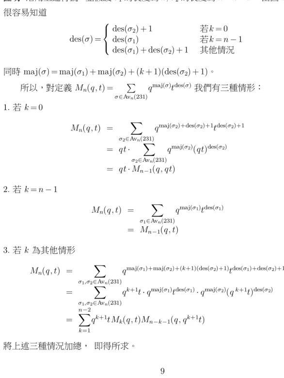
(15) 以及：引理 2.2. (Dokos, Dwyer, Johnson, Sagan, Selsor [6]) 對任一 σ ∈ Sn, 我們有： maj σ = c. #. n 2. $. − maj σ. 其中 σ c 是 σ 的補 (complement)，即若 σ = σ1σ2...σn, 則 σ c = (n + 1 − σ1), (n + 1 − σ2). , ..., (n + 1 − σn)。 Stump 建構出一種複雜的雙射證明下列定理，對六種 S3 的配對都成立。如果我們只需要證明 (Avn(123), Avn(321)) 一種情形則不需要如此大費周章，直接用引理 2.2 就可以得到。定理 2.3. (Stump [17]) !. q. maj (σ) imaj(σ). t. =. σ∈Avn(123). !. !. q. n 2. ". −maj (σ). !. t. n 2. ". −imaj(σ). σ∈Avn(321). 其中 imaj(σ) = maj(σ −1)。. 2.2 定理 1.1 的證明我們先證明 σ ∈ Avn(231) 若且唯若 σ = 132[σ1, 1, σ2], 如圖 2.2 所示，且 σ1 和 σ2 都屬於某長度的 231-有禁排列。證明. 假設 σ ∈ Avn(231), 並且寫成 σ = σlnσr, 其中 σl 和 σr 分別為 σ 中 n 的左邊子序列和右邊子序列。因為 σ ∈ Avn(231), 所以所有 σl 中的元素必定小於 σr 中的元素，因此必定可以寫成 σ = 132[σ1, 1, σ2] 的形式，而且 σl = σ1, σr = σ2。反過來說，如果 σ = 132[σ1, 1, σ2], 且 σ1 和 σ2 都屬於某長度的 231-avoiding。 σ 中若有任意子序列 σiσ jσk 是 231 的模式, 則 σi 和 σk 必定分別屬於 σ1 和 σ2, 否則會和 σ1 和 σ2 都屬於某長度的 231-有禁排列矛盾。但是因為 σ = 132[σ1, 1, σ2], 所以 σ1 中的元素必定都小於 σ2 中的元素，這樣又和 σiσ jσk 是 231 的模式矛盾。因此我們知道，若 σ = 132[σ1, 1, σ2], 且 σ1 和 σ2 是某長度的 231-有禁排列，可得 σ ∈ Avn(231)。. 綜合以上，得知 σ ∈ Avn(231) ⇔ σ = 132[σ1, 1, σ2] and σ1, σ2 ∈ Av(231)。 8. #.

(16) 圖 2.2. σ ∈ Avn(231). 接著我們證明定理 1.1：證明. 沿用上述符號，並假設 σ1 的長度為 k, σ2 的長度為 n − k − 1。由圖 2.2 我們很容易知道. ⎧ ⎨ des(σ2) + 1 des(σ) = des(σ1) ⎩ des(σ1) + des(σ2) + 1. 若k = 0 若k = n − 1 其他情況. 同時 maj(σ) = maj(σ1) + maj(σ2) + (k + 1)(des(σ2) + 1)。 ( 所以，對定義 Mn(q, t) = q maj(σ)tdes(σ) 我們有三種情形： σ∈Avn(231). 1. 若 k = 0. Mn(q, t) =. ). q maj(σ2)+des(σ2)+1tdes(σ2)+1. σ2 ∈Avn(231). = qt ·. ). q maj(σ2)(qt)des(σ2). σ2 ∈Avn(231). = qt · Mn−1(q, qt) 2. 若 k = n − 1 Mn(q, t) =. ). q maj(σ1)tdes(σ1). σ1 ∈Avn(231). = Mn−1(q, t) 3. 若 k 為其他情形 Mn(q, t) = = =. ). σ1,σ2 ∈Avn(231). ). q maj(σ1)+maj(σ2)+(k+1)(des(σ2)+1)tdes(σ1)+des(σ2)+1 q k+1t · q maj(σ1)tdes(σ1) · q maj(σ2)(q k+1t)des(σ2). σ1,σ2 ∈Avn(231) n−2 ) q k+1tMk(q, t)Mn−k−1(q, k=1. 將上述三種情況加總，即得所求。 9. q k+1t) ".

(17) 2.3 用 Maxima 程式進行驗證我們定義 M0(q, t) = 1 和 M1(q, t) = 1, 並用 maxima 驗證定理 1.1 中 Mn(q, t) 的遞迴關係，其中用符號 MQT(n) 表示多項式 Mn(q, t), 而 Mn(q, q kt) 可以用指令 subst 和 MQT(n) 得到，如 subst(q^k*t, t, MQT(n))。關於 MQT(n) 的程式碼請參閱附錄。下表指令 (%i6), (%i8) 和 (%i10) 分別驗證等式當 n = 3, 4, 5 時的情形。 (%i1) batchload("/Users/change/lib.txt")$ (%i2) powerdisp:true$ (%i3) MQT(0); (%o3) 1 (%i4) MQT(1); (%o4) 1 (%i5) MQT(2); (%o5) 1 + q t (%i6) MQT(3)-expand(q*t*(subst(q*t,t, MQT(2)))+MQT(2)+sum((q^(k+1))*t*MQT(k)*subst((q^(k+1))*t,t, MQT(2-k)),k,1,1)); (%o6) 0 (%i7) MQT(3); (%o7) 1 + 2 q t + q 2 t + q 3 t2 (%i8) MQT(4)-expand(q*t*(subst(q*t,t, MQT(3)))+MQT(3)+sum((q^(k+1))*t*MQT(k)*subst((q^(k+1))*t,t, MQT(3-k)),k,1,2)); (%o8) 0 (%i9) MQT(4); (%o9) 1 + 3 q t + 2 q 2 t + q 3 t + 3 q 3 t2 + 2 q 4 t2 + q 5 t2 + q 6 t3 (%i10) MQT(5)-expand(q*t*(subst(q*t,t, MQT(4)))+MQT(4)+sum((q^(k+1))*t*MQT(k)*subst((q^(k+1))*t,t, MQT(4-k)),k,1,3)); (%o10) 0 (%i11) MQT(5); (%o11) 1 + 4 q t + 3 q 2 t + 2 q 3 t + q 4 t + 6 q 3 t2 + 5 q 4 t2 + 6 q 5 t2 + 2 q 6 t2 + q 7 t2 + 4 q 6 t3 + 3 q 7 t3 + 2 q 8 t3 + q 9 t3 + q 10 t4. 10.

(18) 3 在 231-有禁排列中逆序數及右至左極大元數的雙統計量多項式本章主要是利用 Catalan 數的二種組合解釋證明定理 1.2。. 3.1 Catalan 數和 Dyck 路徑 Catalan 數，OEIS 編號 A000108 序列[15], 我們列出開頭的幾項： (c0, c1, c2, ...) = (1, 1, 2, 5, 14, 42, 132, 429, ...) Dyck 路徑是很常見卡特蘭數的組合解釋，長度為 n 的 Dyck 路徑是指在座標平面從 (0, 0) 走到 (2n, 0)，它是由 n 步的上升步 (U) 和 n 步的下降步 (D) 所組成，每個 U 和 D 都可以分別看成座標平面上的 (1,1) 和 (1,-1) 二個向量，並且中途絕對不會低於 x 軸。令 Dn 是所有長度為 n 的 Dyck 路徑所成的集合。. 由於這篇論文主要探討生成函數間的關係，所以我們利用 Catalan 數的生成 1. 函數來得到 cn = n + 1. !. 2n n. ". 這項精確的公式。令 c(z) = c0 + c1z + c2z 2 + ... + cnz n +. ... 是前述 Catalan 數的生成函數，因為生成函數保有四則運算的性質，我們可以由下圖得到：當 n " 1 時，cn = c0cn−1 + c1cn−2 + ... + cn−1c0, 並且由遞迴式得生 √ 1 − 1 − 4z 2 成函數 c(z) 滿足方程式 c(z) = 1 + zc(z) , 解 c(z) = , 對 c(0) = 1 才成立 2z [5]。. 利用 Taylor 多項式 f (x) =. " f (n)(a) (x − a)n 我們可以將二項式定理擴充到對 n! n!0 !. ". m (m − 1) ... (m − n + 1). 任意 m ∈ R 且 n 是非負整數的廣義二項式係數 m = 和廣義二 n! n ! " " m n 項式定理，即 (1 + x)m = x , 參閱文獻 [3, Chapter 4]. 因此我們得到： n n!0. (1 − 4z). 1/2. !# 1/2 $ = (−4z)n n n!0 % & % & ! 1 · 1 − 1 · ... · 1 − (n − 1) 2 2 2 = 1+ (−4)nz n n! n!1 % & ! 1 − 1 · − 3 · ... · 3 − 2n 2 2 2 = 1+ · (−4)nz n 2n (n − 1)! n!1 ! 1 2n−1 · (1 · 3 · ...(2n − 3)) = 1−2· · zn n (n − 1)! n!1 11.

(19) ! 1 (1 · 3 · ...(2n − 3)) 2n−1 · (n − 1)! · · zn n (n − 1)! (n − 1)! n!1 !1 (2n − 2)! = 1−2· · zn n (n − 1)! · (n − 1)! n!1 ! 1 # 2n − 2 $ = 1−2· · zn n−1 n n!1 ! 1 # 2n $ = 1−2· · z n+1 n n+1 = 1−2·. n!0. 即 1−. √. 1 − 4z = 2 ·. ". " 1 ! 2n " n 1 ! 2n " n+1 z , 二邊同除 2z 可得 c(z) = z 。 n n n!0 n + 1 n!0 n + 1. 3.2 堆疊排序和 Dyck 路徑. Knuth 於 1960 年代研究 Sn 的有禁模式時，提出了堆疊可排序 (stack sortable) 的問題。堆疊 (stack) 是一個後進先出的序列，並且在開口的位置藉由推 (push) 和拉 (pop) 二種動作來增減項目。我們稱排列 σ = σ1 σ2 ...σn 為堆疊可排序排列是指 σ 的元素經過堆疊操作可排成遞增序列 123...n。 Bona 在 [2] 中描述 Knuth 的這個操作：推和拉的操作符合貪求演算法 (greedy algorithm), 即只有在推一個 σ 的元素進入堆疊中會違反「堆疊裡的元素必須保持從上到下遞增」這個條件時，我們才從堆疊中拉一個元素出來。如圖 3.1 是以上述條件重新排序 σ = 32154 的一個例子：. 圖 3.1. s(32154) = 12345. 令 s(σ) 是上述程序的輸出，且 σ = LnR ∈ Sn, 其中 L 表示 σ 中 n 左邊的. ，R 則代表 n 右邊的. 串. 串。若 σ 為堆疊可排序，我們可以很容易由上述程序得. 到 s(σ) = s(L)s(R)n, 其中 L 中的最大元素小於 R 中最小的元素。Knuth 在 [9] 中得到堆疊可排序排列的刻畫：定理 3.1. 排列 σ ∈ Sn 是堆疊可排序排列，若且唯若 σ ∈ Avn(231)。 12.

(20) 我們想把 231-有禁排列對應到 Dyck 路徑上，可以利用前面提到的堆疊排序方式：每個推的操作以 1 表示，每個拉的操作以 0 表示。則排列 σ ∈ Avn(231) 可表示成 n 個 1 和 n 個 0 組成的序列，令此序列為 p = p1 p2...p2n，並且滿足條件：對於任一長度 k(1 ! k ! 2n) 的初始序列 p1 p2...pk, 1 元素的個數恆大於等於 0 元素的個數。如圖 3.1 中，我們把 σ = 32154 對應到 ψ(σ) = p = 1110001100。我們可以令 1→上升步, 0→下降步, 將 p 畫成 Dyck 路徑. 。. 3.3 定理 1.2 的第一種證明首先我們定義二個 Dyck 路徑上的統計量：對於 Dyck 路徑的相鄰二步 pipi+1 , 若 (pi , pi+1) = (1, 0) = (U , D), 則稱 pipi+1 為山峰(peak), 用 pk(p) 來表示路徑 p 的山峰數；相反的，若 (pi , pi+1) = (0, 1) = (D, U ), 則稱 pipi+1 為山谷(valley), 用 val( p) 來表示路徑 p 的山谷數。Dyck 路徑和直線 y = 0 圍出的面積 (area), 用 area(p) √ √ 來表示，要注意的是此處的單位面積必須是完整的 2 × 2 正方形。例：若 σ = 2137465 ∈ Av7(231), 使用前一章堆疊排序的演算法得到 σ 的 Dyck. 路徑 p = 11001011011000 如圖 3.2 所示，從圖中我們可以很容易計算 pk(p) = 4, 而 area(p) = 5.. 圖 3.2. Dyck 路徑的山峰和面積. 在圖 3.2 中可以觀察出，所有的山峰都出現在 p 中 (1, 0) 的位置。這代表在排序時 σi (i 此時是山峰的位置)被推進堆疊後直接拉出。由於貪求演算法的特性，代表 σi < σi+1, 又 σi < σ j ∀i + 1 ≤ j ≤ n, 否則 σi σi+1 σ j 就會形成 231 的模式。所以我們可以說 σi 此時是 σ 的一個右到左極小元素，Dyck 路徑中每一個山峰都貢獻一個右到左極小元素，因此 rlmin(σ) = pk(p)。我們把 Dyck 路徑上的每一步標上對 σ 操作的元素。可以發現，當把 σ j 拉出堆疊時，還留在堆疊中的元素 σi 必定滿足 i < j 且 σi > σ j 。又對 σ j 而言，堆疊中 σi 的個數，等於 σi 所貢獻的左逆序，並且和 σ j 在 Dyck 路徑中代表的下降步結束位置的高度(level)相同，而此高度恰好是 σi 下降步貢獻的面積，因此我們斷定 inv σ = area(p). 13.

(21) 由 Cn(q, t) 的定義我們可得： ! ! Cn(q, t) = q inv(σ)trlmin(σ) = q area(P )tpk(P ). (3.1). P ∈Dn. σ∈Avn(231). 現在我們從 Dyck 路徑 P 第一次回到 x 軸的位置將 P 分解成 P = UQDR, 其中 Q 是長度為 k(0 ! k ! n − 1) 的 Dyck 路徑，R 是長度為 n − k − 1 的 Dyck 路徑。. 以下我們給出定理 1.2 的第一種證明。證明. 觀察下列二種情形： 1. 如果 Q = ∅, 則 P = UDR, area(P ) = area(R), pk(P ) = pk(R) + 1, 因此 ! ! Cn(q, t) = q area(P )tpk(P ) = q area(R)tpk (R)+1 = tCn−1(q, t) P ∈Dn. R∈Dn−1. 2. 如果 Q = / ∅, 則 P = UQDR, area(P ) = area(Q) + k + area(R), pk(P ) = pk(Q) +pk(R), 因此. Cn(q, t) =. !. q area(P )tpk(P ) =. P ∈Dn. n−1 !. q area(Q)+area(R)+ktpk(Q)+pk (R). k=1. =. n−1 !. q kCk(q, t)Cn−k−1(q, t). k=1. 由 (3.1) 式與上述二種情形合起來即是我們所求的遞迴關係。. #. 3.4 定理 1.2 的第二種證明二元樹 (rooted binary tree) 也是常見 Catalan 數的組合解釋之一。我們使用 [13] 中的方法來證明我們的遞迴式。二元樹是指資料結構中，每個節點 (node) 最多有二個子點，分別為左子點與右子點。將排列 σ ∈ Avn(231) 以遞迴方式表示成. 二元樹 T (σ), 以最大元素 n 為根，設 σn−k = n, 由 σ 的分解 σ = αnβ, 其中 α ≡ σ1σ2 ...σn−k−1 對應根的左子樹，而 β ≡ σn−k+1σn−k+2...σn 對應根的右子樹。. 14.

(22) σ = αnβ 滿足下列條件： i. 對所有 α 中的元素 σi 與 β 中的元素 σ j 而言，σi < σ j 。 ii. α ∈ Avn−k −1(231) 且 β ∈ Avk(231)。對 α 和 β 重複以上的步驟，我們可以得到一個二元樹。圖 3.3 的二元樹就是 σ = 321549687∈Av7(231) 的例子，σ 可以藉由投射的方式對應回到水平軸上。. 圖 3.3. 一個二元樹與 231-有禁排列. 我們可以藉由底下二個表格顯示出. ". q inv(σ)trlmin(σ) 對應的二元樹分類. σ∈Av4(231). 方式是：所有節點的右子點總數與右子樹為空的節點數。 q 6t 4321. q 2t2 2143. q 3t2 1432 3214. q 4t2 4132 4213. q 5t2 4312. qt3 1243 1324 2134. q 2t3 1423 3124. q 3t3 4123. 表 3.1. 長度為 4 的 231-有禁排列分別對 inv(σ) 和 rlmin(σ) 的分佈. 表 3.2. 二元樹的細分. 15. t4 1234.

(23) 和[13]中的假設不同的是：我們用最大值來分解 σ, 而不是最小值。觀察統計量的對應，我們發現： i. σ 的下降數 des(σ) 等於樹 T (σ) 中右子樹非空的頂點個數，因此我們得到 des(σ) = des(α) + des(β) + χ(β = / ∅). (3.2). 其中 χ(“條件”) 定義為如果 “條件” 為真則為 1 否則為 0。 ii. σ 的元素所貢獻的右逆序數，等於樹 T (σ) 中根的右子樹的頂點個數，因此我們有 inv(σ) = inv(α) + inv(β) + k. (3.3). iii. 因為 σ ∈ Avn(231), 所以 rlmin(σ) = n − des(σ)。證明. 如果我們定義： Cn(q, t) =. !. q inv(σ)trlmin(σ). σ∈Avn(231). 對 σ ∈ Avn(231), 我們有下列二種情形： 1. 如果 k = 0, β = ∅, 由 (3.2) 及 (3.3) 式，我們有 des(σ) = des(α) 且 rlmin(σ) = n − des(α) = n − (n − 1 − rlmin(α)) = rlmin(α) + 1, 因此 Cn(q, t) =. !. q inv αtrlmin(α)+1 = tCn−1(q, t). α∈Avn(231). 2. 如果 k = / 0, 由 3.2 及 3.3 式，我們有 des(σ) = des(α) + des(β) + 1 且 rlmin(σ) = n − (des(α) + des(β) + 1) = rlmin(α) + rlmin(β), 因此 !. Cn(q, t) = = =. α,β ∈Avn(231). !. q inv(α)+inv(β)+k · trlmil(α)+rlmil(β) q k(q inv(α)trlmil(α))(q inv(β)trlmil(β)). α,β ∈Avn(231) n−1 ! q kCk(q, t)Cn−k−1(q, t) k=1. 將二種情形合起來即是我們所求的遞迴關係。 16. #.

(24) 3.5 用 Maxima 程式進行驗證我們用與上一章相同的想法來驗證，此處符號 CQT(n) 表示多項式 Cn(q, t) ，其中指令 (%i9) 驗證等式當 n = 6 時的情形。關於 CQT(n) 的程式碼請參閱附錄。 (%i1) batchload("/Users/change/lib.txt")$ (%i2) powerdisp:true$ (%i3) CQT(0); (%o3) 1 (%i4) CQT(1); (%o4) t (%i5) CQT(2); (%o5) q t + t2 (%i6) CQT(3); (%o6) q 3 t + 2 q t2 + q 2 t2 + t3 (%i7) CQT(4); (%o7) q 6 t + q 2 t2 + 2 q 3 t2 + 2 q 4 t2 + q 5 t2 + 3 q t3 + 2 q 2 t3 + q 3 t3 + t4 (%i8) CQT(5); (%o8) q 10 t + 2 q 4 t2 + 3 q 6 t2 + 2 q 7 t2 + 2 q 8 t2 + q 9 t2 + 3 q 2 t3 + 5 q 3 t3 + 4 q 4 t3 + 5 q 5 t3 + 2 q 6 t3 + q 7 t3 + 4 q t4 + 3 q 2 t4 + 2 q 3 t4 + q 4 t4 + t5 (%i9) CQT(6)-expand(t*CQT(5)+sum((q^k)*CQT(k)*CQT(5-k),k,1,5)); (%o9) 0 (%i10) CQT(6); (%o10) q 15 t + q 6 t2 + 2 q 7 t2 + 2 q 9 t2 + 2 q 10 t2 + 3 q 11 t2 + 2 q 12 t2 + 2 q 13 t2 + q 14 t2 + q 3 t3 + 6 q 4 t3 + 6 q 5 t3 + 7 q 6 t3 + 7 q 7 t3 + 9 q 8 t3 + 6 q 9 t3 + 5 q 10 t3 + 2 q 11 t3 + q 12 t3 + 6 q 2 t4 + 10 q 3 t4 + 9 q 4 t4 + 9 q 5 t4 + 8 q 6 t4 + 5 q 7 t4 + 2 q 8 t4 + q 9 t4 + 5 q t5 + 4 q 2 t5 + 3 q 3 t5 + 2 q 4 t5 + q 5 t5 + t6. 17.

(25) 4 Dyck 路徑和 231-有禁排列本章我們另外介紹二種將 231-有禁排列與 Dyck 路徑的雙射對應關係，可以方便的解釋前一章中 Avn(231) 中 inv(σ) 和 rlmin(σ) 與 Dn 中 area(P ) 和 pk(P ) 之間的對應關係，並且得到：定理 4.1. 若 ψ: Avn(231) → Dn 為前述堆疊排序的雙射對應，則對 σ ∈ Avn(231), des(σ) = dr(ψ(σ)) = n − rlmin(σ) 其中 dr(σ) 定義為 Dyck 路徑中雙升(double rise)的數量，分佈方式為 Narayana 數。. 4.1 Stump 的雙射對應我們將排列中相鄰二元素的轉置 (i, i + 1), 1 ! i < n 記做 si。Stump 在[18]中給出一個將 Dyck 路徑雙射對應到 231-有禁排列的方法。. 圖 4.1. 將長度為 6 的 Dyck 路徑對應到簡單的轉置. 我們將長度為 n 的 Dyck 路徑下的每個單位面積分層依序標號，每一層的單位面積上依序標上 s1s2...sn−ℓ, 其中 ℓ 代表第 ℓ 層。這樣我們有 n − 1 個排列得到 X1X2...Xn−1，此處的 Xℓ 有可能為空. 串依序. 串。如圖 4.1 所示，二個轉置的. 合成由右而左作用，例如：s1s2s3s4s5|s1s2s4|s1 ◦ 123456 = 632154 = σ ∈ Av6(231)。若 φ 為將 Dyck 路徑對應到 231-有禁排列的方法，則對 P ∈ Dn, σ = φ(P ) 而言， s1|s4s2s1|s5s4s3s2s1 ◦ σ 與 3.2 節中所敘述的堆疊排序 s(σ) = s(L)s(R)n 等價，而且. inv(σ) = area(P )。我們注意到對連續的 mi, 1 ! mi ! n − 1, sm1sm2...smi 相當於輪換 (m1, m2, ..., mi , mi + 1), 如圖 4.1 的 s1s2s3s4s5s1s2s4s1 寫成輪換的形式為 (123456) (123)(45)(12)，而每個這種形式的輪換都貢獻一個下降數，而在 Dyck 路徑中 sm1 相應的單位面積左邊的角必然對應到一個雙升 18. 的位置。此外也很容易觀.

(26) 察出第一個山峰的高度剛好是 s1 的數量 +1。. 4.2 將 231-有禁排列的下降段對應到 Dyck 路徑 Petersen 在 [11, Chapter 2] 中建構一雙射函數 ψ: Avn(231) → Dn, 如下圖：. 圖 4.2. 由 231-有禁排列的下降段建構的 Dyck 路徑. 將 σ ∈ Avn(231) 的每個下降段(decreasing runs) σi > σi+1 > ... > σ j 依序放入 n × n 的棋盤方格中，其中第 i 欄(由左而右)第 j 列(由下而上)定義為 (i, j)。給定一個 σ = σ1σ2...σn, 在 (i, σi) 填入 σi, 如圖 4.2。若 σ ∈ Avn(231), 則 σ 所對應的 Dyck 路徑為以 σ 的右到左極小元素為山峰，從 (0, 0) 到 (n, n), 由向右步與向上步構成，且途中不會走到直線 y = x 上方的 Dyck 路徑。ψ −1: Dn → Avn(231) 的方式如下：給定一條本節定義 Dyck 路徑的棋盤，從最右邊山峰的格子放上西洋棋的城堡，在該列不能再有其他的棋子，由右向左在每一行放上城堡，如果該行不是 Dyck 路徑的山峰，則城堡放在該行 Dyck 路徑上方，可以放到最低的列，城堡的位置 (i , σi) 得到的排列 σ = σ1σ2...σn ∈ Avn(231)。由這個雙射對應，可以觀察出 rlmin(σ) =pk(ψ(σ))，並且有如下性質：性質 4.2. (Petersen [11]) 對任一 σ ∈ Avn(231), P = ψ(σ) 而言，滿足 des(σ) = n − 1 − val(P ) = n − pk(P ) 現在我們將前述的 Dyck 路徑以直線 y = x 鏡射後，順時針旋轉 45◦, 可以發現 19.

(27) 正是圖 3.2, 而雙射函數 ψ 也正是我們在第 3 章中所描述的堆疊排序演算法。並且由 des(σ) = dr(ψ(σ)) 得到定理 4.1。. 圖 4.3. 將 Dyck 路徑以直線 y = x 鏡射. 4.3 其他的一些性質我們也可以試著求出 Dyck 路徑中雙升統計量的生成函數。假設 Dyck 路徑每單位長度用一個 z 代表，每個雙升用一個 t 表示，生成函數為 C(t, z):. 圖 4.4. 雙升統計量. 圖 4.4 中 t 點必然. 在，當 t 之後為 C(t, z) − 1 時，所以我們可以得到： C(t, z) = 1 + zC(t, z) + zt (C(t, z) − 1)C(t, z). 解 C(t, z) 可得 C(t, z) =. 1 + z(t − 1) −. '. 1 − 2z(t + 1) + z 2(t − 1)2 2tz. (4.1). 4.1 式和 [11, Chapter 2] 中 Dyck 路徑上山峰統計量的分佈同為 Narayana 數。. 20.

(28) 5 未來研究方向我們提出二個未來研究的方向作為論文的結尾。 a) 第 4 章的討論可以看成 [19] 中紀錄 Narayana 數的一種解釋。我們知道，下降數在 Sn 中是 Eulerian 數，但是在有禁排列中卻成為 Narayana 數。Petersen 在 [11]中為我們介紹了這二者都有 γ-非負 (γ-nonnegative) 的性質。由於 γ-非負在研究對稱數列的一種特殊性質，理論上除了 Catalan 數有關的數列外，Motzkin 數、Schröder 數...等等的相關數列，還有哪些數列擁有此種性質？問題 5.1. (Petersen [11]) 對 n > 0, 找出數列 Pn(t) 滿足下列條件： Pn(t) =. ⌊(n−1)/2⌋ !. γn,jtj (1 + t)n−1−2j. j=0. 其中 γn,j 為非負整數。. b) 第 3、4 章中，我們對連結 231-有禁排列與 Dyck 路徑的堆疊排序方法分別用三種不同的方法加以描述。而在研究的文獻中，231-有禁排列和 Dyck 路徑分別可以用不同的方法連結非交叉分拆(noncrossing partition)。Blanco 和 Petersen 在 [1] 中曾提出一個問題：問題 5.2. (Petersen [1]) 是否可以找到統計量 st(σ) 使得 !. q area(P )trank(P ) =. P ∈Dyck(n). !. q ℓ(σ)tst(σ) ?. σ∈Avn(231). 此處 rank(P ) 為非交叉分拆直接對應 Dyck 路徑所賦予的。. Blanco 和 Petersen 使用了在 Sn 中各種 Eulerian 數的統計量，都沒有結果。我們嘗試了本篇論文中的五種 Sn 中的 Stirling 數的統計量，也都不符合分佈： D4(q, t) = 1 + 3qt + 2q 3t + q 5t + 3q 2t2 + 2q 4t2 + q 6t2 + q 3t3 D5(q, t) = 1 + 4qt + 6q 2t2 + 3q 3t + 2q 5t + q 7t + 6q 4t2 + 5q 6t2 + q 8t2 + q 10t2 + 4q 3t3 +3q 5t3 + 2q 7t3 + q 9t3 + q 4t4 也許需要從其他類型統計量尋找。. 21.

(29) 參考文獻 [1] S. A. Blanco and T. K. Petersen. Counting Dyck paths by area and rank. Annals of Combinatorics, 18(2):171–197, (2014). [2] M. Bóna. A survey of stack-sorting disciplines. Electronic Journal of Combinatorics, 9(2):A1, (2002-3). [3] M. Bóna. A Walk Through Combinatorics: An Introduction to Enumeration and Graph Theory (3rd Edition). World Scientific Publishing, Singapore, 2011. [4] S.-E. Cheng, S. Elizalde, A. Kasraoui, and B. E. Sagan. Inversion polynomials for 321-avoiding permutations. Discrete Mathematics, 313(22):2552–2565, (2013). [5] M. Delest. Algebraic languages: a bridge between combinatorics and computer science. DIMACS Series in Discrete Mathematics and Theoretical Computer Science , 24:71–88, (1996). [6] T. Dokos, T. Dwyer, B. P. Johnson, B. E. Sagan, and K. Selsor. Permutation patterns and statistics. Discrete Mathematics, 312(18):2760–2775, (2012). [7] J. Fürlinger and J. Hofbauer. q-Catalan numbers. Journal of Combinatorial Theory , 40(2):248–264, (1985). [8] F. Hirzebruch. Eulerian polynomials. Münster Journal of Mathematics, pages 9–14, (2008). [9] D. E. Knuth. The Art of Computer Programming, Vol. 1: Fundamental Algorithms, 3rd ed . Addison Wesley, Reading, Massachusetts, 1997. [10] L. M. Lai and T. K. Petersen. Euler-mahonian distributions of type Bn . Discrete Mathematics, 311:645–650, (2011). [11] T. K. Petersen. Eulerian Numbers. Birkhäuser/Springer, New York, 2015. [12] S. Poznanović. The sorting index and equidistribution of set-valued statistics over restricted permutations. Journal of Combinatorial Theory, Series A, 125:254–272, (2014). [13] D. Rawlings. Bernoulli trials and permutation statistics. International Journal of Mathematics and Mathematical Sciences, 15(2):291–311, (1992). [14] R. Simion and F. W. Schmidt. Restricted permutations. European Journal of Combinatorics, 6(4):383–406, (1985). [15] N. J. A. Sloane. On-line encyclopedia of integer sequences. https://oeis.org/. [16] R. P. Stanley. Enumerative Combinatorics, Vol. 1 and Vol. 2 . Cambridge University Press, Cambridge/New York, 1997, 1999. [17] C. Stump. On bijections between 231-avoiding permutations and Dyck paths. arXiv:0803.3706, (2008). [18] C. Stump. More bijective Catalan combinatorics on permutations and on signed permutations. Journal of Combinatorics, 4(4):419–447, (2013). [19] R. A. Sulanke. Catalan path statistics having the Narayana distribution. Discrete Mathematics, 180(1-3):369–389, (1998).. 22.

(30) /* Appendix */ /* I save this to the file lib.txt and include it first when I want verify the polynomial in my master thesis */ /* The number of inversions for a permutation P */ inv(P):= block( [i,j,n,number], n:length(P), i:1, number:0, while i<=n-1 do ( j:i+1, while j<=n do ( if P[j]<P[i] then number:number+1, j:j+1 ), i:i+1 ), number )$ /* The number of descents for a permutation P */ des(P):= block( [i,n,number], n:length(P), i:1, number:0, while i<=n-1 do ( if P[i]>P[i+1] then number:number+1, i:i+1 ), number )$ /* The number of left-to-right maximum for a permutation P */ lrmax(P):= block( [i,j,n,number,flag:1], n:length(P), i:2, number:1, while i<=n do ( j:1, while j<=i-1 and flag=1 do ( if P[i]<P[j] then flag:0, j:j+1 ), if flag=1 then number:number+1,. 23.

(31) flag:1, i:i+1 ), number )$ /* The number of right-to-left minimum for a permutation P */ rlmin(P):= block( [i,j,n,number,flag:1], n:length(P), i:1, number:1, while i<=n-1 do ( j:i+1, while j<=n and flag=1 do ( if P[i]>P[j] then flag:0, j:j+1 ), if flag=1 then number:number+1, flag:1, i:i+1 ), number )$ /* The major index for a permutation P */ maj(P):= block( [i,n,id], n:length(P), i:1, id:0, while i<=n-1 do ( if P[i]>P[i+1] then id:id+i, i:i+1 ), id )$ /* Major index distributions on S_n */ MQ(n):= block( [T,Q,x], T: permutations(makelist(i,i,1,n)), Q: 0, for x in T do (Q: Q+q^maj(x)), Q )$ /* The number of inversions distributions on S_n */ IQ(n):=. 24.

(32) block( [T,Q,x], T: permutations(makelist(i,i,1,n)), Q: 0, for x in T do (Q: Q+qînv(x)), Q )$ /* The number of inversions distributions on S_n(231) */ CQ_hat(n):= block( [T,Q,x], T: S231(n), Q: 0, for x in T do (Q: Q+qînv(x)), Q )$ /* (inversion,rlmin)-joint distributions on S_n(231) */ CQT(n):= block( [T,Q,x], if n=0 then return (1), T: S231(n), Q: 0, for x in T do (Q: Q+qînv(x)*t^rlmin(x)), Q )$ /* (major,descent)-joint distributions on S_n(231) */ MQT(n):= block( [T,Q,x], T: S231(n), Q: 0, for x in T do (Q: Q+q^maj(x)*t^des(x)), Q )$ /* The following functions test S_3 by 231-pattern */ TEST231(P):= block( [i,j,k,n,flag:0], n:length(P), i:1, while i<=n-2 and flag=0 do ( j:i+1, while j<=n-1 and flag=0 do ( if P[j]>P[i] then ( k:j+1,. 25.

(33) while k<=n and flag=0 do ( if P[k]<P[i] then flag:1, k:k+1 ) ), j:j+1 ), i:i+1 ), flag )$ /* The following functions return 231-avoiding permutation with legth=n */ S231(n):= block( [i,S,L,x], S: permutations(makelist(i,i,1,n)), L: {}, for x in S do (if TEST231(x)=0 then L:adjoin(x,L)), L )$. 26.

(34)