檢定多重擾動以偵測微弱相關

國立臺灣大學公共衛生學院流行病學與預防醫學研究所 博士論文

Institute of Epidemiology and Preventive Medicine College of Public Health

National Taiwan University Doctoral Dissertation

檢定多重擾動以偵測微弱相關

Detecting a Weak Association by Testing its Multiple Perturbations

羅敏子 Min-Tzu Lo

指導教授：李文宗 教授

Advisor: Wen-Chung Lee, MD, PhD

中華民國 102 年 7 月 July, 2013

i

Contents

口試委員會審定書 ... iv

誌 謝 ... v

中文摘要 ... vi

ABSTRACT ... vii

I. INTRODUCTION ... 1

II. THE TRADITIONAL METHOD... 3

III. THE MULTIPLE PERTURBATION TEST ... 5

IV. POWER COMPARISON... 7

V. MONTE-CARLO SIMULATION ...11

VI. APPLICATION TO REAL DATA ... 15

VII. DISCUSSION ... 19

REFERENCE ... 23

APPENDIX 1 ... 27

APPENDIX 2 ... 29

ii

Figure and Table Contents

Figure 1. Powers of the multiple perturbation test for the sharp null (solid lines, theoretical power assuming independent auxiliary variables with perturbation proportion of, from left to right respectively,

1.0, 0.2, 0.1 and 0.05) and the conventional test for the crude null (dashed line), under different number of subjects (panel A:

, panel B:

=1000

n

, panel C:

) and number of auxiliary variables. ...10 Figure 2. Empirical powers of the multiple perturbation test with panels of

independent and dependent auxiliary variables (circle: empirical power for independent auxiliary variables; triangle: empirical power for mildly dependent auxiliary variables; square: empirical power for strongly dependent auxiliary variables)...13 Figure 3. Fixation (panels A-C, respectively for the 1

to the 3

top single

nucleotide polymorphisms, SNPs) and drifting (panels D-F, for three

purposefully chosen middle-to-bottom ranking SNPs) of the P-values

of the multiple perturbation test when only a certain number of

perturbation SNPs are incorporated for the age-related macular

degeneration data.

Each panel includes three lines (solid, dashed and

dotted) representing three random incorporation sequences. Each

P-value is obtained from 1000000 rounds of permutation. ...18

iii

Figure 4. Power curve when a researcher includes the 100 informative variables (

) known to him/her and then other low-informativity variables (dotted lines from left to right, for

0.0001 and 0.00025 0.001,

=

I

, respectively) unselectively into the

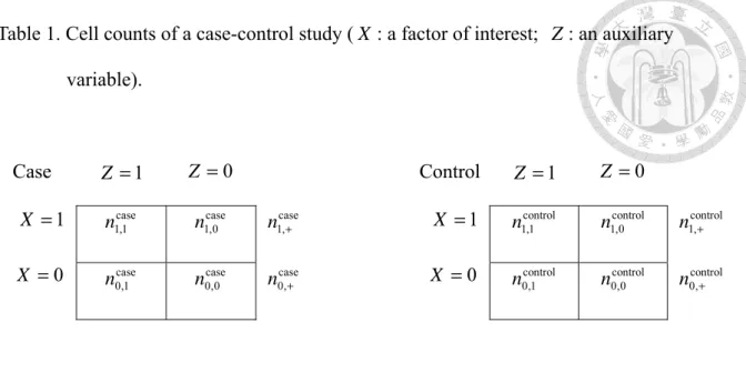
multiple perturbation test. ...22 Table 1. Cell counts of a case-control study (

: a factor of interest;

: an

auxiliary variable). ...4 Table 2. Type I error rates of the multiple perturbation test with panels of

independent and dependent auxiliary variables...14 Table 3. Top five single nucleotide polymorphisms (SNPs) with smallest

P-values by the multiple perturbation tests for the age-related macular

degeneration data. ...17

iv

口試委員會審定書

v

誌 謝

首先，最感謝指導教授李文宗老師六年來的教導，每次跟老師討論，總是有許多收 穫，對於老師清晰的邏輯、敏捷的思緒和敏銳的洞察力，都為之讚嘆！老師對於研究的 熱忱和專注力，都是我學習的目標。還要感謝口試委員黃景祥老師、蕭朱杏老師、程毅 豪老師、杜裕康老師和洪弘老師，謝謝老師們提供的寶貴建議，對於論文的完整性給予 很大的幫助。

謝謝一起奮鬥了六年的博士班同學們杞蓉、秋霞、亭誼和世亨，今年我們四個女生 一起畢業了，還有李老師研究室的同學們筱元、齡誼、紫婷、德恩、薏竹、紫渲，一起

出國開會的季侑、淑芬，一起在544 室努力的夥伴們，和碧華學姊。特別還要謝謝我的

家人對我的包容與支持，感謝大家的陪伴，讓我這六年的研究生活，充滿了許多值得回 憶的事。

vi

中文摘要

在流行病學和生物醫學研究中，許多危險因子或介入的效應非常微小。為了偵測這 些微小的效應，研究必須要具有大樣本數，也就是研究個案要夠多。研究者當然可以增 加樣本數，但是有其限制。在這篇論文中，我們提出一個嶄新的方法，以不同方向來增 加樣本數，也就是增加變項數量(p)。我們建構一個以 p 為本的「多重擾動檢定」，並且

進行理論統計檢力計算和電腦模擬。當p 非常大時，如數千甚至數百萬，多重擾動檢定

可以達到很高的統計檢力來偵測微弱的效應。我們還應用多重擾動檢定來重新分析一個 已經發表的老年性黃斑部病變的全基因體相關性研究。我們找出兩個和疾病相關而且新

的顯著基因。這個以p 為本的多重擾動檢定，相信在未來，可以樹立一個新的統計上假

設檢定的典範。

關鍵字：假設檢定、交互作用、錯誤發現率、老年性黃斑部病變、跨體學研究、資料探 勘

vii

ABSTRACT

Many risk factors/interventions in epidemiologic/biomedical studies are of minuscule effects. To detect such weak associations, one needs a study with a very large sample size (the number of subjects, n). The n of a study can of course be increased but only to an extent. In this paper, the authors propose a novel method which hinges on increasing sample size in a different direction—the total number of variables (p). The authors construct a p-based

‘multiple perturbation test’, and conduct theoretical power calculations and computer simulations to show that it can achieve a very high power to detect weak associations when p can be made very large, say, to the thousands or millions. The authors apply the method to re-analyze a published genome-wide association study on age-related macular degeneration and identify two novel genetic variants that are significantly associated with the disease. The p-based method may set a stage for a new paradigm of statistical hypothesis tests.

Keywords: hypothesis testing; interaction; false discovery rate; age-related macular degeneration; cross-omics study; data mining.

1

I. INTRODUCTION

Many risk factors/interventions in epidemiologic/biomedical studies are of minuscule effects.¹ For example, television viewing was found to increase the risks of type 2 diabetes, cardiovascular disease and all-cause mortality, but the effects in terms of relative risks are small: 1.20, 1.15 and 1.13,² respectively; regular supplement of vitamin C was associated with a shortening of the duration of common colds, but with a relative risk (0.92) very near unity.³ Moving into this ‘–omics’ era, for the first time researchers are becoming able to probe into study subjects’ genome, transcriptome, and metabolome, etc, to search for possible disease associations. However, the associations found so far were still very weak; for example the great majority of the odds ratios of genetic polymorphisms in genome-wide association studies were less than 1.5.^4,5

To detect weak associations, a very large sample size is needed. For example, in genome-wide association studies, the sample sizes have steeply increased from a few hundreds in the first study of age-related macular degeneration⁶ to tens of thousands in recent meta-analyses.^7,8 Also, the consortium-based studies are becoming increasingly indispensible as the single-institution studies often cannot meet the tough sample-size requirements. For example, the Wellcome Trust Case-Control Consortium⁹, the United Kingdom Biobank¹⁰ and China Kadoorie Biobank¹¹ have recruited study subjects in the order of hundreds of thousands. But how big is big enough for sample size? A simulation study suggested that in some scenarios the sample size needed can easily go up to the millions!¹² Certainly, there is a limit for the total number of subjects any research institution, any meta-analysis and any consortium can possibly assemble.

Traditionally, sample sizes are measured in terms of the total number of study subjects (n). In this study, we propose a novel ‘p-based’ method which hinges on increasing sample size in a different direction—the total number of variables ( p ).We

2

construct a p-based ‘multiple perturbation test’, and conduct theoretical power calculations and computer simulations to show that it can achieve a very high power to detect a weak association when p can be made very large, say, to the thousands, millions or even more. We will also apply the new method to re-analyze a published genome-wide association study.⁶

3

II. THE TRADITIONAL METHOD

Assume that we are interested in the association between a binary factor, X (X = 1 indicates a subject is exposed to the factor, X =0, otherwise) and a disease, D (D= 1 indicates a subject is diseased, D=0, otherwise). The traditional n-based method tests whether the disease risk varies with X in the study population as a whole, i.e., testing the

‘crude’ null, H^crude₀ : Pr( | ) Pr( )D X = D , against the alternative, H₁^crude: Pr( | ) Pr( ).D X ≠ D In a case-control study conducted in the study population, Appendix 1 shows that testing the crude null amounts to testing the equality of prevalence odds of X , between the case group (Odds^case_X ) and the control group (Odds^control_X ) (or equivalently, testing whether the odds ratio of X and D equals one: ORcase-control_XD =Oddscase_X Oddscontrol_X = ). Table 1 presents the 1 cell counts of a case-control study (ignore the variable, Z , for now). One may use the following test statistic:

{ } { }

1 . 1

log log

Odds log Var Odds

log Var

Odds log Odds

log

0,1 0,1 control

, case

,

2

control , 0 control

, 1 case

, 0 case

, 1

control case

control 2 case

2 crude

 

∈ + ∈ +

+ + +

+

∧

∧

∧

∧

+











 −

=



 

 + 



 







 



 −

=

j j j j

X X

X X

n n

n n n

n

χ

2 crude

χ is distributed asymptotically as a chi-squared distribution with one degree of freedom (df) under the crude null.

4

Table 1. Cell counts of a case-control study ( X : a factor of interest; Z : an auxiliary variable).

Case Z =1 Z =0 Control Z =1 Z =0

=1

X _n1,1^case _n1,0^case _n1,^case₊ X =1 _n1,1^control _n1,0^control _n1,^control₊

=0

X n_0,1^case n_0,0^case n^case_0,+ X =0 n_0,1^control n_0,0^control n_0,^control₊

5

III. THE MULTIPLE PERTURBATION TEST

Consider a binary auxiliary variable, Z (Z =1 or 0), which is not of direct interest to us, but may help discern the possible association between X and D . Our proposed method is based on testing whether the disease risk varies with X in any segment of the population demarcated by Z , i.e, testing the ‘sharp’ null, H^sharp₀ : Pr( | , ) Pr( | )D X Z = D Z for both

=1

Z and Z =0, against the alternative, H^sharp₁ : Pr( | , ) Pr( | )D X Z ≠ D Z for either Z =1 or Z =0.

In a case-control study conducted in the study population, Appendix 1 shows that testing the sharp null amounts to testing the equality of odds ratios of X and Z , between the case group (OR^case_XZ ) and the control group (OR^control_XZ ) (or equivalently, testing whether there is an

‘interaction’ between X and Z with regard to the risk of D on a multiplicative scale:

case control

OR_XZ OR_XZ = ). The following test statistic is proposed (see Table 1 for the cell counts): 1

{ } { }

1 , 1

log

OR log Var OR

log Var

OR log OR

log

0,1

, , 0,1 control

, case

,

2

control 1 , 0 control

0 , 1

control 0 , 0 control

1 , 1 case

1 , 0 case

0 , 1

case 0 , 0 case

1 , 1

control case

control 2 case

2 sharp

 

∈ ∈

∧

∧

∧

∧

+













×

− ×

×

×

=



 

 + 



 







 



 −

=

k

j jk jk jk

XZ XZ

XZ XZ

n n

n n

n n

n n

n n

χ

which is distributed asymptotically as a df 1= chi-squared distribution under the sharp null.

Essentially, χ_sharp² is testing whether the observed

case

ORXZ

∧ and

control

ORXZ

∧ are being

‘perturbed’ too much away from OR^population_XZ (the population odds ratio of X and Z , and

the expected value for both

case

ORXZ

∧ and

control

ORXZ

∧ under the sharp null) than chance alone would dictate. We therefore refer to it as a ‘perturbation test’.

One single auxiliary variable may not perturb the above odds ratios very much. But if one has a whole panel of auxiliary variables (the Z and the corresponding _i χ_{sharp, i}² , for

6

1, 2,...,

i= p), one can construct a very powerful multiple perturbation test, by summing up the perturbations from the many auxiliary variables (Zs) in the panel:

2 sharp, 1

.

p

p i

i

T χ

=

=



T as such is a p-based test. Its power to detect a non-null X should increase as more p Zs are included in the panel (as p increases). On the other hand, a truly innocent X should be able to stand the test from multiple Zs, even if p goes to infinity. If the Zs in the panel are independent of one another, T is asymptotically a df_p = chi-squared p

distribution under the sharp null. The critical value of T therefore is simply _p χ_df²= p_,1−_α

when the level of significance is set at α .

In actual practice however, one often cannot assume independent Zs and therefore has to rely on computer-intensive methods to simulate the null sampling distribution of T . With _p

1

p= , Buzkova et al. ¹³ pointed out that the method of parametric bootstrap is valid but the method of permutation (shuffling disease status between subjects) is conservative (overestimating the critical value). However, we found that as p increases, the permutation method remains slightly conservative but the parametric method becomes too liberal (underestimating the critical value). To err on the safe side, we therefore propose to use the permutation method to approximate the null sampling distribution of T . _p

7

IV. POWER COMPARISON

The power of the traditional n-based χ_crude^{2 is:}

2 2 2

crude df 1 df 1, 1 α

Power of χ ≈Prχ = ( )λ >χ = − ,

where χ_{df 1}²₌ ( )λ ^{is a df 1}= noncentral chi-squared distribution with noncentrality

parameter,

( )

( )

{ } ^{{ }}

( )

case control 2

case control

0,1 , 0,1 ,

logOdds logOdds

1 1

E E

X X

j nj j nj

λ

∈ + ∈ +

= −

 +  . Note that the power of χ_crude² is determined

by the significance level: ,α the sample size: n (or more exactly the expected cell counts), and the effect size: logOdds^case_X −logOdds^control_X .

Assuming that a panel of independent auxiliary variables contains a certain proportion, (0 1)

π ≤ ≤ , of perturbative π ^Zs such that ^{log OR}

(

)

2 df ,1 2

df 2

Power of Pr ,

1

p

p p

T χ ^α

χ θ

= −

=

 

≈  > + 

where

( )

( )

{ }

2 2

case control

, 0,1 , , 0,1 ,

1 1 .

E E

j k nj k j k nj k

θ π σ

∈ ∈

= ×

 +  Note that in addition to α and ⁿ, the

power of T is also determined by the total number of auxiliary variables: _p p , and the

‘informativeness’ of the auxiliary variables: I = ×π σ² (the product of perturbation proportion and perturbation strength).

We consider an X that is very weakly associated with D (ORcase-control_XD =Oddscase_X Oddscontrol_X =1.1). We also consider a panel of independent Zs. The

8

logarithm of OR^population_XZ follows a normal distribution with a mean of zero and a variance of 0.5 (a probability of 95% that an OR^population_XZ is between 0.25 ~ 4.00). We consider four different values for the perturbation proportion (π =1.0, 0.2, 0.1 and 0.05, respectively), with each perturbative Z having a weak perturbation strength (σ² =0.001, i.e., a probability of 95% that the ratio, OR^case_XZ OR^control_XZ , is between 0.94 ~ 1.06). The informativeness of Zs is therefore 0.001, 0.0002, 0.0001 and 0.00005, respectively. For convenience, the prevalence of

X and each and every one of Zs is set at 40% for the control group. The significance level is set at α =0.05.

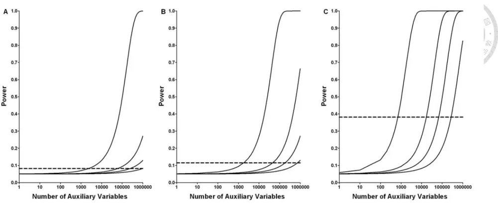
Figure 1 compares the theoretical powers of T (the multiple perturbation test for the _p sharp null, solid lines) and χ_crude² (the conventional test for the crude null, dashed lines) in three different sample sizes (total number of subjects, n) of 500 (250 cases₊250 controls, panel A), 1000 (500₊500, panel B) and 5000 (2500₊2500, panel C). The four solid lines in each panel correspond to different perturbation proportions (from left to right: π =1.0, 0.2, 0.1 and 0.05, respectively). It can be seen that, indeed, the power of the n-based χ_crude² increases with n. However, the increment is marginal at best; the power gain is only 30%, from 8% (n=500, panel A) to 38% (n=5000, panel C). In fact, we need a very large study (n=~ 15000) to attain an adequate power of 80% for the χ_crude² test (not shown in the figure). On the other hand, the power of the p-based T increases with p in all scenarios _p that we considered and surpasses the power of χ_crude^{2 when p}≈³⁰⁰⁰ for π =1 ,

60000

p≈ for π =0.2, 250000p≈ for π =0.1 and p≈1000000 for π =0.05. Under

=1

π , the power of T can reach nearly 100% when p is sufficiently large _p ( p>~1000000 when n=500 ; p>~100000 when n=1000 ; p>~10000 when

9 5000

n= ). Under π <1, ~100% power is also possible if p can be made even larger.

10

Figure 1. Powers of the multiple perturbation test for the sharp null (solid lines, theoretical power assuming independent auxiliary variables with perturbation proportion of, from left to right respectively, π =1.0, 0.2, 0.1 and 0.05) and the conventional test for the crude null (dashed line), under different number of subjects (panel A: n=500, panel B: n=1000, panel C: n=5000) and number of auxiliary variables.

11

V. MONTE-CARLO SIMULATION

In this section, we perform Monte-Carlo simulation to study the statistical properties of

T empirically. The parameter setting is the same as the previous section. But to avoid the p

heavy computation burdens of simulating a very large panel of Zs, this time we let Zs to have a perturbation proportion of 1.0 and a larger perturbation strength (σ² =0.004, a probability of 95% that OR^case_XZ OR^control_XZ is between 0.88 ~ 1.13). Additionally, we also consider dependent Zs. Specifically, we simulate Zs using a first-order Markov chain, in both the case and the control groups, assuming an odds ratio between successive Zs of 2.0 (mild dependency) and 5.0 (strong dependency), respectively. We perform a total of 1000 simulations. In each round of the simulation, we conduct 1000 permutations to obtain an empirical P-value for T . The power of _p T is then calculated as the proportion of the _p simulations with aP-value 0.05.<

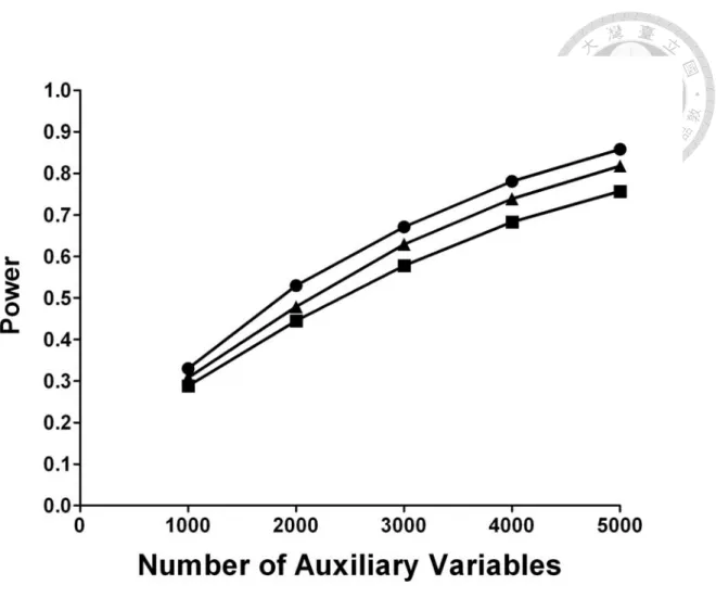
Figure 2 shows the empirical powers of T for panels of independent and dependent _p s

Z at different number of auxiliary variables ( p ) when sample size is n=1000. As compared to independent Zs, at the same p the empirical power does compromise a bit for mildly dependent Zs, and yet a bit more for strongly dependent Zs. However, the overall trend is clear: the empirical power increases as p increases, irrespectively of using independent, mildly or strongly dependent Zs. Thus, to make up for the power loss in using dependent Zs, one can simply include more Zs in the panel.

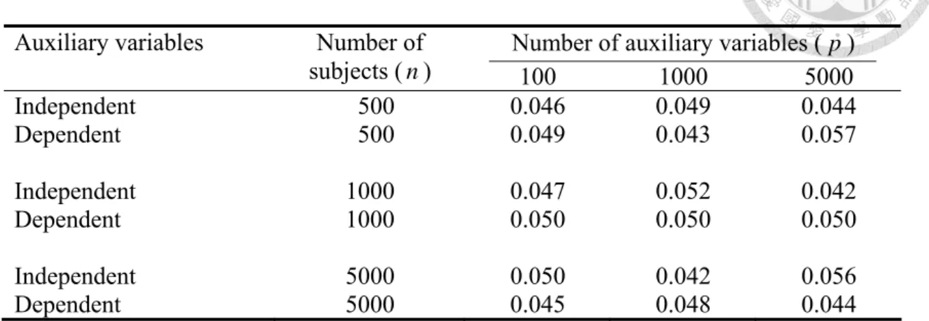
The type I error rates of T for panels of independent and dependent _p Zs (odds ratio between successive Zs 5.0= ) are also empirically checked using Monte-Carlo simulations, for different number of subjects (n=500,1000,5000) and number of auxiliary variables (p=100,1000,5000). Here X is a sharp null, that is, X has no effect on disease in any

12

level stratified by Zs (no perturbation effect for all Z s: I = ×π σ² = ). Other parameters 0 are the same as in the previous power simulations. We perform a total of 1000 simulations, each round with 1000 permutations. The results are shown in Table 2. We see that the T _p test can maintain quite accurate type I error rates for all scenarios considered.

13

Figure 2. Empirical powers of the multiple perturbation test with panels of independent and dependent auxiliary variables (circle: empirical power for independent auxiliary variables; triangle: empirical power for mildly dependent auxiliary variables;

square: empirical power for strongly dependent auxiliary variables).

14

Table 2. Type I error rates of the multiple perturbation test with panels of independent and dependent auxiliary variables.

Auxiliary variables Number of Number of auxiliary variables ( p )

subjects (n) 100 1000 5000

Independent 500 0.046 0.049 0.044

Dependent 500 0.049 0.043 0.057

Independent 1000 0.047 0.052 0.042

Dependent 1000 0.050 0.050 0.050

Independent 5000 0.050 0.042 0.056

Dependent 5000 0.045 0.048 0.044

15

VI. APPLICATION TO REAL DATA

The proposed multiple perturbation test is applied to a public-domain data from a genome-wide association study of age-related macular degeneration.⁶ The study recruited 146 individuals (96 cases and 50 controls) and genotyped 116212 single nucleotide polymorphisms (SNPs). A total of 6639 SNPs located in chromosome 1 (where previous studies^14,15 have identified a number of significant susceptibility genes) with call rate>95%, minor allele frequency>5% and in Hardy-Weinberg equilibrium in the control group is included in the analysis. At each SNP, heterozygote and variant homozygote are grouped together.

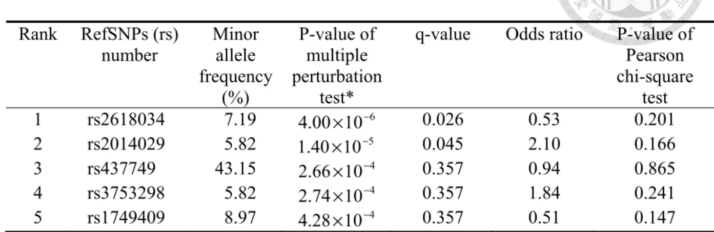
In the analysis, each SNP takes turn to be the X , and the remaining SNPs, the s.Z There are a total of C⁶⁶³⁹₂ =22034841 perturbations (interactions) to be considered. (For a low-frequency SNP, some of the cells in Table 1 may be empty. In that case, it is totally uninformative as a perturbation variable, because its χ_sharp² statistic is zero with the convention: 0 log 0 0× = .) The P-value of the multiple perturbation test for each SNP is obtained from 500000 rounds of permutation. To adjust for multiple testing, the false discovery rate (FDR) is controlled at 0.05 and the q-values are calculated (QVALUE software).¹⁶ Table 3 lists the top five SNPs with smallest P-values by the multiple perturbation tests. The multiple perturbation test detects two significant SNPs at FDR of 0.05:

rs2618034 (q-value= 0.026) and rs2014029 (q-value = 0.045).

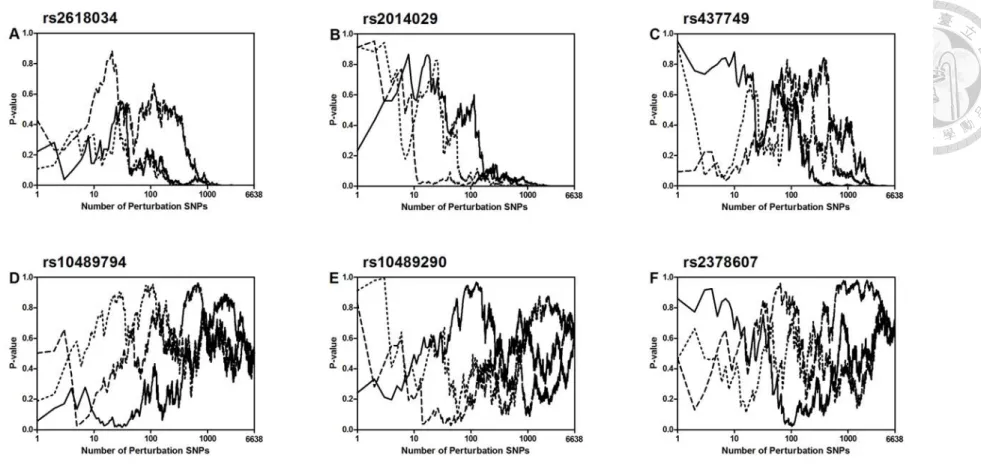
In the above analysis, for each SNP all the remaining 6638 SNPs are incorporated as perturbation variables into the multiple perturbation test. Figure 3 shows the P-values of the multiple perturbation test when only a certain number of perturbation SNPs are incorporated.

Each panel of the figure plots the results of three random incorporation sequences. Panels A-C are for the 1^st to the 3^rd top SNPs, respectively. We see that initially the P-values

16

fluctuate a lot, when the number of perturbation SNPs incorporated is small. But beyond a certain point, the P-values become ‘fixed’ exactly to the abscissa (P-values= 0) (Panels A and B), or almost fixed to the abscissa (P-values≈0) (Panel C). By comparison, we see that the P-values of all three purposefully chosen middle-to-bottom ranking SNPs are ‘drifting’ all the way without showing any sign of a fixation (Panels D-F). It is worth noting that although the 3^rd top SNP (rs437749) is not significant by our FDR standard (Table 3), it is already displaying a fixation pattern in our fixation/drifting analysis (Figure 3C). This suggests that if we can incorporate more perturbation SNPs into the multiple perturbation test, SNP rs437749 may become significant.

For the two significant SNPs found in this study, it is of interest to examine whether the significances are due primarily to the perturbations from one or a few other SNPs. We deliberately remove the respective five largest χ_{sharp, i}² ’s in the multiple perturbation tests for these two SNPs. The result for rs2618034 is still highly significant (P-value₌6×10⁻⁶; q-value₌0.038), and that for rs2014029, marginally so (P-value₌ 2.8×10⁻⁵; q-value₌0.090).

In fact, even if we remove the respective ten largest χ_{sharp, i}² ’s of the two SNPs, a clear fixation pattern can still be seen for both (Appendix 2).

17

Table 3. Top five single nucleotide polymorphisms (SNPs) with smallest P-values by the multiple perturbation tests for the age-related macular degeneration data.⁶

Rank RefSNPs (rs)

number Minor allele frequency

(%)

P-value of multiple perturbation

test*

q-value Odds ratio P-value of Pearson chi-square

test 1 rs2618034 7.19 4.00×10⁻⁶ 0.026 0.53 0.201 2 rs2014029 5.82 1.40×10⁻⁵ 0.045 2.10 0.166 3 rs437749 43.15 2.66×10⁻⁴ 0.357 0.94 0.865 4 rs3753298 5.82 2.74×10⁻⁴ 0.357 1.84 0.241 5 rs1749409 8.97 4.28×10⁻⁴ 0.357 0.51 0.147

*based on 500000 rounds of permutation

18

Figure 3. Fixation (panels A-C, respectively for the 1^st to the 3^rd top single nucleotide polymorphisms, SNPs) and drifting (panels D-F, for three purposefully chosen middle-to-bottom ranking SNPs) of the P-values of the multiple perturbation test when only a certain number of perturbation SNPs are incorporated for the age-related macular degeneration data.⁶ Each panel includes three lines (solid, dashed and dotted) representing three random incorporation sequences. Each P-value is obtained from 1000000 rounds of permutation.

19

VII. DISCUSSION

While confronted with high-throughput data, researchers often turn to dimension reduction methods of sorts to ease the severe penalty associated with testing myriads of variables.^17-21 For our p-based method, dimensionality is not a curse but in fact is a blessing.

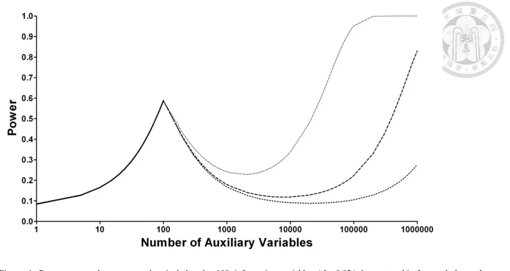
In this paper, we see that the power of the multiple perturbation test actually increases as the number of auxiliary variables increases. Such ‘the-more-the-better’ principle also applies, when one is knowledgeable about which variables may be perturbative. In Figure 4, the initial segment of the power curve (solid line) emulates a situation when a researcher incorporates into the multiple perturbation test the total 100 informative variables (I =0.02) that are known to him/her. Since the power is only 0.59, should the researcher add more variables into the test? We see as expected that adding more variables unselectively (dotted lines from left to right, for I =0.001,0.00025 and 0.0001, respectively) into the test will only dilute the power. However, upon more and more of these low-informativity variables being added, the power then rises up again and surpasses the original power.

However, it should be emphasized that the above p-based approach only goes so far as when the auxiliary variables have a non-zero informativeness (I >0, irrespectively of how small it may be). A computer can easily generate millions and billions of random variables for us, but all these artificial data amount to nothing (I =0, exactly). The more such variables being added, the more the power will be curtailed. Another caveat is that there is no use replicate the data at hand just to make the total number of auxiliary variables appear larger;

the power simply won’t bulge with this maneuver.

Age-related macular degeneration is a progressive disease in macula of the retina in which the pigment epithelium cells and the photoreceptor cells degenerate, causing gradual loss of central vision.^22,23 With FDR controlled at 0.05, in this study we are able to identify

20

two novel SNPs that are significantly associated with age-related macular degeneration. The first SNP (rs2618034) is located in the intron region of KCND3 gene (potassium voltage-gated channel, Shal-related subfamily, member 3) on chromosome 1p13.2, and the second (rs2014029), the intron region of DTL gene (denticleless E3 ubiquitin protein ligase homolog (Drosophila)) on 1q32.3. KCND3 gene encods Kv4.3 regulating neuronal excitability.²⁴ Mutations in KCND3 gene have been identified as a cause for cerebellar neurodegeneration.^25,26 In this regard, it is worthy to note that the retina photoreceptor cells are a specialized type of neurons which may also degenerate with aging. Meanwhile, DTL gene regulates p53 polyubiquitination and protein stability²⁷ and the evidence to date suggests that p53 is a key regulator involved in the apotosis of retinal pigment epithelium cells.²⁸ All these findings further support that KCND3 and DTL genes may be causally related to the development of age-related macular degeneration.

It is worthy to note that the proposed p-based multiple perturbation test indeed is a very powerful test. The two significant SNPs (rs2618034 and rs2014029) that we identified in this study are only very weakly associated with age-related macular degeneration (odds ratios= 0.53 and 2.10, respectively), and the traditional n-based method (Pearson chi-square test) comes nowhere near detecting them (P-values= 0.201 and 0.166, respectively) (Table 3).

Even if we increase the total number of subjects from the present n=146(Klein et al’s data⁶) to n≈25000 and n≈77000 (Holliday et al’s⁷ and Fritsche et al’s⁸ meta-analyses data), the n-based method still cannot detect them. But this is not to say that the n-based method is useless. In fact, Klein et al⁶ themselves presented one SNP (rs380390) with an n-based P-value of 4.1 10× ^-8 (significance after Bonferroni correction), but it is undetectable with our method. It is important to note that the p-based test proposed in this paper is not meant to take the place of the traditional n-based test. It is better that they can work side by side,

21

complementing each other. Finally, we wish to point out that by incorporating a priori knowledge into analyzing Klein et al’s data,⁶ Lin and Lee²⁹ previously were able to identify four more significant SNPs in chromosome 1 (rs800292, rs2019727, rs1329428 and rs1853882) using the traditional n-based test. The same principle can also be applied to the p-based multiple perturbation test in this paper to facilitate the detection of even more genes.

In this paper, we have successfully applied the multiple perturbation test to a genome-wide association study where thousands of genomic markers serve the roles of the auxiliary/perturbation variables. The method should have broad applications to other high-dimension (large p ) -omics studies, such as epigenomic, transcriptomic, proteomic, metabolomic, and exposomic studies, etc. It would be even better to have a cross-omics study, and/or with all its study subjects further linked to existing government or private-sector databases, such as, data of health insurances, traffic violations, internet usages, etc. A researcher conducting such a data-mining study has the potentials to push the p (the number of auxiliary/perturbation variables) to the millions, billions or even trillions, and be rewarded with a very high power for detecting a weak association. Such a p-based method may set a stage for a new paradigm of statistical hypothesis tests.

22

Figure 4. Power curve when a researcher includes the 100 informative variables (I =0.02) known to him/her and then other low-informativity variables (dotted lines from left to right, for I =0.001,0.00025 and 0.0001, respectively) unselectively into the multiple perturbation test.

23

REFERENCE

1. Siontis, G.C., and Ioannidis, J.P. (2011). Risk factors and interventions with statistically significant tiny effects. Int J Epidemiol 40, 1292-1307.

2. Grontved, A., and Hu, F.B. (2011). Television viewing and risk of type 2 diabetes, cardiovascular disease, and all-cause mortality: a meta-analysis. JAMA 305, 2448-2455.

3. Hemila, H., and Chalker, E. (2013). Vitamin C for preventing and treating the common cold.

Cochrane Database Syst Rev 1, CD000980.

4. Ioannidis, J.P., Trikalinos, T.A., and Khoury, M.J. (2006). Implications of small effect sizes of individual genetic variants on the design and interpretation of genetic association studies of complex diseases. Am J Epidemiol 164, 609-614.

5. Hindorff, L.A., Sethupathy, P., Junkins, H.A., Ramos, E.M., Mehta, J.P., Collins, F.S., and Manolio, T.A. (2009). Potential etiologic and functional implications of genome-wide association loci for human diseases and traits. Proc Natl Acad Sci U S A 106, 9362-9367.

6. Klein, R.J., Zeiss, C., Chew, E.Y., Tsai, J.Y., Sackler, R.S., Haynes, C., Henning, A.K., SanGiovanni, J.P., Mane, S.M., Mayne, S.T., et al. (2005). Complement factor H polymorphism in age-related macular degeneration. Science 308, 385-389.

7. Holliday, E.G., Smith, A.V., Cornes, B.K., Buitendijk, G.H., Jensen, R.A., Sim, X., Aspelund, T., Aung, T., Baird, P.N., Boerwinkle, E., et al. (2013). Insights into the genetic architecture of early stage age-related macular degeneration: a genome-wide association study meta-analysis. PLoS One 8, e53830.

8. Fritsche, L.G., Chen, W., Schu, M., Yaspan, B.L., Yu, Y., Thorleifsson, G., Zack, D.J., Arakawa, S., Cipriani, V., Ripke, S., et al. (2013). Seven new loci associated with age-related macular degeneration. Nat Genet 45, 433-439, 439e431-432.

24

9. Wellcome Trust Case Control, C. (2007). Genome-wide association study of 14,000 cases of seven common diseases and 3,000 shared controls. Nature 447, 661-678.

10. Ollier, W., Sprosen, T., and Peakman, T. (2005). UK Biobank: from concept to reality.

Pharmacogenomics 6, 639-646.

11. Chen, Z., Chen, J., Collins, R., Guo, Y., Peto, R., Wu, F., Li, L., and China Kadoorie Biobank collaborative, g. (2011). China Kadoorie Biobank of 0.5 million people: survey methods, baseline characteristics and long-term follow-up. Int J Epidemiol 40, 1652-1666.

12. Chapman, K., Ferreira, T., Morris, A., Asimit, J., and Zeggini, E. (2011). Defining the power limits of genome-wide association scan meta-analyses. Genet Epidemiol 35, 781-789.

13. Buzkova, P., Lumley, T., and Rice, K. (2011). Permutation and parametric bootstrap tests for gene-gene and gene-environment interactions. Ann Hum Genet 75, 36-45.

14. Lim, L.S., Mitchell, P., Seddon, J.M., Holz, F.G., and Wong, T.Y. (2012). Age-related macular degeneration. Lancet 379, 1728-1738.

15. Gorin, M.B. (2012). Genetic insights into age-related macular degeneration: controversies addressing risk, causality, and therapeutics. Mol Aspects Med 33, 467-486.

16. Storey, J.D., and Tibshirani, R. (2003). Statistical significance for genomewide studies. Proc Natl Acad Sci U S A 100, 9440-9445.

17. Chatterjee, N., Kalaylioglu, Z., Moslehi, R., Peters, U., and Wacholder, S. (2006). Powerful multilocus tests of genetic association in the presence of gene-gene and gene-environment interactions. Am J Hum Genet 79, 1002-1016.

18. Gauderman, W.J., Murcray, C., Gilliland, F., and Conti, D.V. (2007). Testing association between disease and multiple SNPs in a candidate gene. Genet Epidemiol 31, 383-395.

19. Wang, T., Ho, G., Ye, K., Strickler, H., and Elston, R.C. (2009). A partial least-square

25

approach for modeling gene-gene and gene-environment interactions when multiple markers are genotyped. Genet Epidemiol 33, 6-15.

20. Pan, W. (2009). Asymptotic tests of association with multiple SNPs in linkage disequilibrium. Genet Epidemiol 33, 497-507.

21. Pan, W. (2010). Statistical tests of genetic association in the presence of gene-gene and gene-environment interactions. Hum Hered 69, 131-142.

22. Bhutto, I., and Lutty, G. (2012). Understanding age-related macular degeneration (AMD):

relationships between the photoreceptor/retinal pigment epithelium/Bruch's membrane/choriocapillaris complex. Mol Aspects Med 33, 295-317.

23. Ambati, J., and Fowler, B.J. (2012). Mechanisms of age-related macular degeneration.

Neuron 75, 26-39.

24. Tsaur, M.L., Chou, C.C., Shih, Y.H., and Wang, H.L. (1997). Cloning, expression and CNS distribution of Kv4.3, an A-type K+ channel alpha subunit. FEBS Lett 400, 215-220.

25. Lee, Y.C., Durr, A., Majczenko, K., Huang, Y.H., Liu, Y.C., Lien, C.C., Tsai, P.C., Ichikawa, Y., Goto, J., Monin, M.L., et al. (2012). Mutations in KCND3 cause spinocerebellar ataxia type 22. Ann Neurol 72, 859-869.

26. Duarri, A., Jezierska, J., Fokkens, M., Meijer, M., Schelhaas, H.J., den Dunnen, W.F., van Dijk, F., Verschuuren-Bemelmans, C., Hageman, G., van de Vlies, P., et al. (2012).

Mutations in potassium channel kcnd3 cause spinocerebellar ataxia type 19. Ann Neurol 72, 870-880.

27. Banks, D., Wu, M., Higa, L.A., Gavrilova, N., Quan, J., Ye, T., Kobayashi, R., Sun, H., and Zhang, H. (2006). L2DTL/CDT2 and PCNA interact with p53 and regulate p53 polyubiquitination and protein stability through MDM2 and CUL4A/DDB1 complexes.

Cell Cycle 5, 1719-1729.

26

28. Bhattacharya, S., Chaum, E., Johnson, D.A., and Johnson, L.R. (2012). Age-related susceptibility to apoptosis in human retinal pigment epithelial cells is triggered by disruption of p53-Mdm2 association. Invest Ophthalmol Vis Sci 53, 8350-8366.

29. Lin, W.Y., and Lee, W.C. (2010). Incorporating prior knowledge to facilitate discoveries in a genome-wide association study on age-related macular degeneration. BMC Res Notes 3, 26.

27

APPENDIX 1

Let 1R= indicate a subject is recruited in a study, R=0, otherwise. In a case-control study, the recruitment process depends only on the disease status of a subject, that is,

Pr(R=1 , , ) Pr(Z X D = R=1 , ) Pr(X D = R=1 ).D Under the crude null of Pr( | ) Pr( )D X = D , we have

Pr( , , 1)

Pr( , 1)

Pr( , 1)

Pr( ) Pr( ) Pr( 1 , )

Pr( ) Pr( 1 ) Pr( ) Pr( ) Pr( 1 )

Pr( ) Pr( 1 ) Pr( ),

X D R X D R

D R

X D X R X D

D R D

X D R D

D R D

X

= = =

=

× × =

= × =

× × =

= × =

= and therefore,

case

population

control

Pr( 1 1, 1)

Odds Pr( 0 1, 1)

Pr( 1)

Pr( 0) Odds

Pr( 1 0, 1)

Pr( 0 0, 1)

Odds .

X

X

X

X D R

X D R

X X

X D R

X D R

= = =

= = = =

= =

=

=

= = =

= = = =

=

Under the sharp null of Pr(D Z X, ) Pr(= D Z), we have Pr( , , , 1)

Pr( , , 1)

Pr( , , 1)

Pr( ) Pr( ) Pr( , ) Pr( 1 , , )

Pr( ) Pr( ) Pr( 1 , ) Pr( ) Pr( ) Pr( ) Pr( 1 )

Pr( ) Pr( ) Pr( 1 )

X Z D R Z X D R

X D R

X Z X D Z X R Z X D

X D X R X D

X Z X D Z R D

X D X R D

= = =

=

× × × =

= × × =

× × × =

= × × =

Pr( ) Pr( )

, Pr( )

Z X D Z

D X

= ×

28

and therefore,

case Pr( 1 1, 1, 1) Pr( 0 1, 1, 1)

OR Pr( 1 0, 1, 1) Pr( 0 0, 1, 1)

Pr( 1 1) Pr( 1 1) Pr( 0 1) Pr( 1 0)

Pr( 1 1) Pr( 1 1)

Pr( 1 0) Pr( 1 1)

Pr( 1 0)

XZ

Z X D R Z X D R

Z X D R Z X D R

Z X D Z Z X D Z

D X D X

Z X D Z

D X

= = = = = = = =

= = = = = = = = =

 = = × = =   = = × = = 

 = =   = = 

   

=  = = × = = 

 = =



population

Pr( 0 0) Pr( 1 0)

Pr( 1 0)

Pr( 1 1) Pr( 0 1)

Pr( 1 0) Pr( 0 0)

OR

Pr( 1 1) Pr( 0 1) Pr( 0 1) Pr( 0 0)

Pr( 0 1) Pr( 0 1)

Pr(

XZ

Z X D Z

D X

Z X Z X

Z X Z X

Z X D Z Z X D Z

D X D X

 = = × = = 

  = = 

  

= = = =

= = = = =

=

 = = × = =   = = × = = 

 = =   = = 

   

=

control

1 0) Pr( 0 1) Pr( 0 0) Pr( 0 0)

Pr( 0 0) Pr( 0 0)

Pr( 1 1, 0, 1) Pr( 0 1, 0, 1)

Pr( 1 0, 0, 1) Pr( 0 0, 0, 1)

OR_XZ .

Z X D Z Z X D Z

D X D X

Z X D R Z X D R

Z X D R Z X D R

 = = × = =   = = × = = 

 = =   = = 

   

= = = = = = = =

= = = = = = = = =

=

29

APPENDIX 2

Fixations of the P-values of the two significant SNPs (rs2618034 and rs2014029) found in this study, even with the respective ten largest χ_{sharp, i}² ’s being removed: