國立臺灣大學電機資訊學院電機工程學研究所 碩士論文
Graduate Institute of Electrical Engineering
College of Electrical Engineering and Computer Science National Taiwan University
Master Thesis
具備低能量消耗之公平獎勵的整合策略
A fair-rewarded aggregation policy for energy saving in IoT
楊鈞皓 Chun-Hao Yang
指導教授:王勝德 博士 Advisor: Sheng-De Wang, Ph.D.
中華民國 106 年 12 月 December 2017
誌謝
首先感謝王勝德老師這兩年對我的指導,也願意在我研究不順利的時候幫我 寫推薦信讓我有這個機會參加交換學生計畫。謝謝實驗室同學振皓與世泓各種研 究上的討論與鼓勵,當然也包括研究外的。謝謝余家菁學姊在我遇到各種疑難雜症 的時候總是願意傾聽與突破盲點,或不吝一記棒喝。
中文摘要
叢集演算法常被使用來產生長時效的網路拓樸,因為這些算法的隨機性和動 態調整,收發封包的工作量會被整個網路的節點所均攤。然而,真正使能耗降低的 因素是資料的整合,從而使傳輸與接收的資料量降低。並且,資料整合策略可以確 保大部分的資料在等待整合的過程中,不至於超過其資料的有效時間。大部分的資 料整合策略在設計時,沒有考慮到網路的拓樸或路由結構,但是這兩者跟資料整合 策略的效能與參數是高度相關的,如離終點有幾個中繼站和接收封包的速度。
本論文提出一個新的基於叢集算法特性的資料整合策略,以達到更好的能源 效率以及更低的資料超時率。透過預測資料超時的情況,我們的方法分析並計算即 將過期與獲得的資料,最後決定傳輸的時間點。實驗模擬的結果顯示,我們花在傳 輸的電力比第二好的算法低上大約 10%到 40%,並且大部分只有 0.5%到 5%的資 料過期率。
關鍵字:資料聚集; 無線感測網路; 物聯網; 簇集演算法; 能源效率
ABSTRACT
Clustering algorithms are the most common methods to create long lifetime network topologies. Due to the dynamic nature and randomness of clustering algorithms, the workload of transmission and reception can be amortized by different nodes. However, the main idea behind saving energy is that data aggregation compression can reduce the data to transmit, and the data aggregation policy is to ensure that the most data can be aggregated without being expired. Most of the data aggregation policy discusses their mathematical model without concerning topology and routing protocol, but yet the topology and routing is closely related to data aggregation policy performance and its parameter, such as number of hop to the data sink and rate of incoming packets.
This paper proposes a new data aggregation policy utilizing the features of clustering algorithms to better improve energy efficiency and expiration rate. By predicting the expiration of data, our method calculates and compares between the number of expiring and incoming data to decide the moment of transmission. The simulation shows that our transmission energy is 10% to 40% lower than the second best solution and most of the packet drop rate is about 0.5% to 5%.
Keywords: Data aggregation; WSN; IoT; clustering algorithm; energy efficiency
CONTENTS
口試委員會審定書 ... #
誌謝 ... i
中文摘要 ... ii
ABSTRACT ... iii
CONTENTS ... iv
LIST OF FIGURES ... v
LIST OF TABLES ... vi
Chapter 1 Introduction ... 1
Chapter 2 Related works ... 3
2.1 Data aggregation policy ... 3
2.2 Clustering algorithm ... 5
Chapter 3 Proposed model ... 7
3.1 Network model ... 7
3.2 Algorithm design ... 8
3.3 Mathematical model ... 13
Chapter 4 Experimental setup ... 16
4.1 Environments ... 16
4.2 Parameters... 18
Chapter 5 Experimental results ... 22
Chapter 6 Conclusion ... 36
REFERENCES ... 37
LIST OF FIGURES
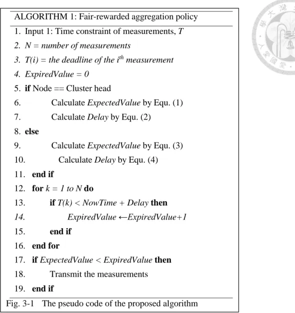
Fig. 3-1 The pseudo code of the proposed algorithm ... 13
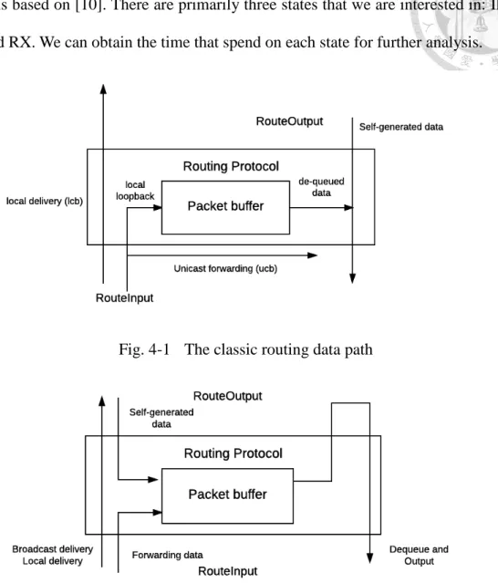
Fig. 4-1 The classic routing data path ... 17
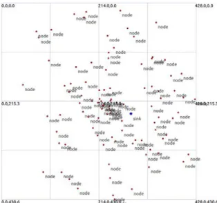
Fig. 4-2 The modified routing data path for data aggregation ... 17
Fig. 4-3 The disc distribution of nodes with radius 225. ... 20
Fig. 4-4 The square distribution of nodes with length 400. ... 20
Fig. 4-5 The square distribution of nodes with length 800 and width 200. ... 20
Fig. 4-6 The small IoT scenario distribution of nodes. ... 21
Fig. 4-7 The big IoT scenario distribution of nodes. ... 21
Fig. 5-1 Energy cost per measurement with lambda, Disc, periodic ... 24
Fig. 5-2 Energy cost per measurement with lambda, Square, periodic ... 25
Fig. 5-3 Energy cost per measurement with lambda, Rectangle, periodic ... 26
Fig. 5-4 Energy cost per measurement with lambda, Disc, Poisson ... 27
Fig. 5-5 Energy cost per measurement with lambda, Square, Poisson ... 28
Fig. 5-6 Energy cost per measurement with lambda, Rectangle, Poisson ... 29
Fig. 5-7 Scalability with different lambda, No policy ... 31
Fig. 5-8 Scalability with different lambda, Proposal ... 31
Fig. 5-9 Scalability with different lambda, OptTM ... 31
Fig. 5-10 Scalability with different lambda, CL ... 32
Fig. 5-11 Transmission moments with 50 nodes and lambda = 1. Orange points are our transmission moments. Gray points are optimal moments mentioned in chapter 3... 32
LIST OF TABLES
Table 5-1. Nodes on Disc topology... 23
Table 5-2. Node drops on Disc topology ... 23
Table 5-3. Nodes on Square topology ... 24
Table 5-4. Node drops on Square topology ... 24
Table 5-5. Nodes on Rectangle topology ... 25
Table 5-6. Node drops on Rectangle topology ... 25
Table 5-7. Nodes on Disc topology... 27
Table 5-8. Node drops on Disc topology ... 27
Table 5-9. Nodes on Square topology ... 28
Table 5-10. Nodes on Square topology ... 28
Table 5-11. Nodes on Rectangle topology ... 29
Table 5-12. Nodes on Rectangle topology ... 29
Table 5-13. IoT scenario experiments, small scale with periodic generation ... 33
Table 5-14. IoT scenario experiments, small scale with Poisson generation ... 34
Table 5-15. IoT scenario experiments, big scale with periodic generation ... 34
Table 5-16. IoT scenario experiments, big scale with Poisson generation ... 34
Chapter 1 Introduction
In the modern development of WSNs, energy efficiency is an important issue since sensors are most deployed in the wild, causing the difficulty of recharging. This results in the development of clustering algorithm, such as LEACH [1], HEED [2], and DEEC [3].
Clustering algorithms select some sensor nodes to be the cluster heads, while others find their nearest cluster heads and become its member. Take LEACH for example. A cluster operates in a periodic manner, which means round after round. In every round, clusters reform by selecting new cluster heads, and the cluster members transmit their sensing data to their nearest cluster heads. With the clustering algorithms, sensor nodes become cluster heads in turn in order to balance the high energy cost of being a cluster head that have an extra energy cost to receive data from cluster members and forward data to the base station. Clustering algorithms have applications in WSN or even IoT environments, such as forest monitoring, modern city services, industrial manufacturing pipeline, etc. In these conditions, cluster heads not only are elected for energy saving purpose, but also can implement some edge computing techniques, e.g. simple statistical works, data compression, or raw data processing. Every nodes including cluster heads and members should generate its sensor data. The sensor data encapsulating with delay requirement as metadata constitute a complete measurement [4]. After a measurement is generated, it is enqueued to the transmission buffer. The non-cluster-head nodes can perform some preliminary operations to refine the packet before transmission, such as concatenate multiple measurements in a packet. In the processing of forwarding the measurements from cluster members, the cluster head can perform data aggregation to remove packet headers and compress the data, further reducing packet size and energy consumption. The
cluster heads therefore have two sources of data incoming, self-sensed and received from cluster members. Both of these measurements are kept in the same buffer to wait for aggregation and transmission. In [5], the authors propose this problem as a tradeoff between energy saving and delay control. In order to save maximum energy, we manage to send the sensor’s data at once, reducing the number of transmission while keeping the maximum number of un-expired data. If more measurements are aggregated in a transmission, some compression techniques can greatly reduce the packet size. The data aggregation policy is the algorithm that determines the moment to transmit the measurements in the buffer.
In this paper, we apply the features of clustering algorithm into the data aggregation policy. Inspired by the application mentioned above, data aggregation policies are highly tended to be implanted in the practical environments. Under the circumstances of WSN, especially the criteria for power limitation, energy consumption is of high importance with regard to packet delay for some delay-insensitive applications. For this purpose, we intend to minimize the energy cost consumed for transmission while tolerating some delay lost.
The rest of the paper is organized as follows. In Section II, we introduce some data aggregation policies. Section III describes the network model and proposing algorithm.
Section IV describes the experiment setup and implementation and section V concludes the paper.
Chapter 2 Related works
2.1 Data aggregation policy
In the history of data aggregation policies, there are a little number of them focused on different aspects to design the aggregation policy in order to achieve energy efficiency.
According to the OSI layer model [9], most of the data aggregation policies focus on the network and the above layer, while some are implemented between the MAC and network layer [12]. Our research includes the LEACH [1] clustering algorithm, which acts as a network layer routing protocol in implementation, and therefore the whole work is constructed upon the network layer. This feature makes the data aggregation policies compatible for this clustering topology since both are based on the network layer. The basic idea behind these aggregation policies is to reduce the number of transmission and concatenate measurements thus decreasing header overhead.
The periodic per hop policy [6] is that each node waits for a predefined interval of time. After the end of the period, sensor nodes transmit all the received and sensed data.
The cascading protocol builds a distribution tree which tells each node that how many hops it is away the sink. The time limitation of the node is determined by the hops away from sink, further the node, shorter the timeout.
Algorithms proposed in [4][7][8] utilize the Markov Decision Process(MDP) model to solve the aggregation problem. A Markov decision process contains states, actions, transition processes, rewards and discount factor. These algorithms define its all these 5 elements with the purpose of maximizing the reward. In [7], the aggregation policy problem is regarded as an optimal stopping problem, which is a subset of stochastic sequential decision problems. A generalized MDP model, semi-Markov decision process
model, is used in [7] to construct the states and its transition distribution. The reward of the model is the aggregation gain, which is application dependent, with exponential decay.
Because the original states are too large for computing, the control limit algorithm is derived by simplifying the possible states to a computable level. This method calculates a threshold of the buffer size. If the buffer size is beyond the threshold, flush the buffer and transmit. Besides the control limit algorithm, two learning methods are proposed for comparison on the aspect of performance and computing complexity. Viewing from another aspect, Arroyo-Valles et al. in [8] gives every measurement an importance as priority, and transmits the measurements based on their importance. Importance is a general evaluation of energy, information source and time constraint. It could result in different performance because of different importance giving policy concerning information from other nodes. Yang et al. encapsulates the data aggregation policy into a transmission manager in [4], and the discussions combine theoretic proof and implementation for realistic scenario. This proposal outstands with a new suggestion that the reward of a measurement should decay linearly rather than exponentially. The solution is derived based on backward induction, a common technique to solve the Markov decision process problems. Since the deployment of WSN sensors should be costly and time-consuming, it is reasonable to share the facility with many applications, resulting with different deadlines. The previous works give decay on reward while it discards the expired measurements in [4]. This brings about the routing hops that should be seriously considered for. Therefore, multi-hop routing scenario is supposed and an enhanced algorithm is introduced.
These algorithms secure data against expiring at the cost of spending more communication energy. The energy efficiency, however, has more space of improvement at some cost of expiration. Our proposed method aims to achieve further energy efficiency
than the existing algorithms.
2.2 Clustering algorithm
LEACH [1] is adopted as the clustering algorithm in our experiments. Although being proposed as clustering algorithm, LEACH can also be implemented as a routing protocol. Some of the other clustering algorithms such as HEED [2] and DEEC [3] are the derivatives of LEACH. LEACH has four phases to consist a round. The first phase is to select the cluster heads in this round. LEACH gives a formula of the threshold, and the nodes generate a random number and compare to the threshold. The cluster heads broadcast their advertisements with the same energy level and the non-cluster-head nodes listen. The second phase is that the non-cluster-head nodes choose the cluster head to join.
After the first phase, the non-cluster-head nodes receive the advertisements from cluster heads. They choose the strongest signal as its source is the closest. The nodes then transmit to the selected cluster head in order to notice the cluster head the member information. The third phase is creating the transmission schedule for every node. In the fourth phase, the nodes transmit their data toward the base station. After these four phases are done, the protocol restarts from the first phase. LEACH wants every node to become cluster head once to share the extra loading of transmission and reception in a big round.
If there is N nodes, and average M cluster heads per round, the big round is comprised of N/M rounds. The node which has become a cluster head should wait until the big round end and the node can become a cluster head again.
For the above algorithms, experiments are made upon simple node distribution, such as linear topology and grid topology. However, in realistic application, the complex topology is different from those in experiments. Suggested that the performance of the
data aggregation policy may be affected by topology, there is an emergent need to discuss aggregation policy on some sophisticated topology, for example, cluster topology such as LEACH.
Chapter 3 Proposed model
In the section, we first introduce the environment on which the aggregation policy algorithm is working. The network model describes the structural elements that surrounds the aggregation policy in the network architecture. These models interact with the aggregation policy directly, and therefore we can have a clear look about the whole network structure. The second part is our proposed algorithm that is aimed to maximize the number of un-expired measurements in a single transmission in order to save energy.
3.1 Network model
From the aspect of the OSI layer model, the data aggregation policy is on the higher layer of the network layer, and is related to the routing function. The policy could change the routing behavior. We can classify incoming packets into two categories: forwarding or arrival. The forwarding packets are not immediately transferred to its next hop. Instead, the packets should wait for the aggregation policy to decide whether to send. If the policy accepts, the measurements in the buffer are aggregated and transmitted. Otherwise, the packets should wait for the next time when the data aggregation policy is triggered. The data aggregation policy checks the packets in the buffer for their time constraints, with the purpose of maximizing the number of un-expired measurements in a single transmission while keeping low expiration rate.
Another important factor is the clustering algorithm. As far as our best knowledge, it is unprecedented to build a data aggregation policy upon a cluster topology. Although named clustering algorithm, this algorithm can also act as a routing protocol, which is on
the same layer of the data aggregation policy. The intertwined structure is further discussed in chapter 4. Speaking from the aspect of a routing protocol, however, the clustering topology is used to collect measurements, and thus is different from the general purposed routing protocol. In a cluster, every node knows its next hop, and is unchanged until the cluster reforms. Every measurement transmitted finally comes to the base station, also called the sink.
The wireless sensor network is originated from the wireless ad-hoc network. In a wireless ad-hoc network, every node can make connection with other nodes, and so can the nodes in the wireless sensor network. With this attribute, we can change the routing path toward the base station by periodically updating the routing table.
3.2 Algorithm design
The main purpose of this data aggregation policy algorithm is to maximize the number of un-expired measurements in a single transmission. To achieve this requirement, we adopt the Markov Decision Process(MDP) [13] model to formulate its behavior and derive the solution. A MDP consists of five elements: states, actions, transition probabilities, rewards, and discount factor. The algorithm is triggered every time when measurements are pushed into the buffer. The below is the five elements of MDP and a table of symbols used in the algorithm and their meanings.
States Sn: the states are defined as the measurements in the buffer. For example, let Sn = (X1, X2, X3), and at the next moment, the node receives a measurement and pushes it to the buffer, the state becomes Sn+1 = (X1, X2, X3, X4). The lower case sn means the number of measurements in the buffer. The subscript n is the order of the state.
Actions An: the model provides two actions, transmit and continue. If the action is "transmit", the buffer is flushed and the measurements are
aggregated and transmitted. The next state becomes empty and restarts from the newly received measurements. If the action is "continue", the buffer remains untouched. There might be some measurements expired waiting for transmission. The buffer can decide whether to drop them in the process of the algorithm.
Transition Probability: P(Sn+1|Sn,An) = 1. The original meaning of this parameter is that given a state and an action, the next state could have more than one outcome. For our case, each action only has one result, no
randomness involves. When the buffer is added with new measurements, the state has to decide its action. The criteria of transmission depend on the reward of the current state and the next state. If the reward of the next state is better than the current, the state would choose to continue. On the other hand, if the next state has less reward, transmission is taken.
Rewards R and discount factor: we define the reward as the number of measurements un-expired. The discount factor is 1 because a measurement is either expired or un-expired, and its corresponding reward is 0 or 1. Maximize the reward, and we can achieve our claim of saving energy by transmitting the most of un-expired measurements in a packet.
Symbol Meaning
Sn The list of measurements in the buffer
sn The number of measurements in the buffer Delay Estimated timing cost of the transmission
T(i) The deadline of the ith measurement in the buffer
ExpiredValue The number of measurements going to be expired at the next moment
ExpectedValue The number of measurements going to be acquired at the next moment
To estimate the reward of the next state, we give the formulation of the expected reward based on some observation. From state Sk to Sk+1, some measurements are pushed to the buffer, while some are expired. The transmission criteria is that the present reward is higher than the reward at the next transmission moment,
Reward(Sn)>Reward(Sn+1). The reward at the next transmission moment is equal to the
present reward plus the ExpectedValue minus the ExpiredValue,
Reward(Sn)>Reward(Sn)+ExpectedValue-ExpiredValue. After some simplification, we
have ExpiredValue>ExpectedValue. The ExpiredValue means the number of measurements that are going to expire in the next moment. The ExpiredValue is
estimated by the time constraint for which we wish to wait and calculates the number of expired measurement before the time constraint. The ExpectedValue represents for the number of coming measurements and is evaluated by sensor generation and forwarding from other nodes.
Assume that we have the measurement generation rate, named λ, and the node's character being as cluster head or cluster member. The cluster members do not receive measurements from others. We analyze the algorithm by cluster head, cluster member, their expected incoming and expired measurements.
A. Cluster head
Expected measurements: The cluster head has additional sources of measurements
by forwarding packets from its cluster member. The cluster head itself generates λ measurements per second, or one measurement per 1/λ second. Once a measurement is generated, the data aggregation policy is triggered. Therefore, the expected value is to calculate the value 1/λ second later. Despite the fact that it is hard to model the
probability when the cluster member is going to forward their measurements, however, it is a simple fact that they all generate one measurements per 1/λ second. We can therefore estimate the number of expected measurements to be the cluster size.
ExpectedValue = 1 + cluster size (1) Expired measurements: The cluster head is only one hop away from its destination,
the base station. After the cluster head decides to transmit, the delay before arriving in the base station is the propagation delay of transmission. The propagation delay is the packet size divided by the wireless traffic rate. However, with only this constraint, our expiration rate would be incredibly high, losing the meaning of sensor deployment. We assign the time which the cluster head takes waiting for transmission to be the buffer size divided by the packet generation rate (λ). This means the time needed to generate the buffer size measurements and the difference of the generation time between the first and the last measurement.
Delay = Prop. delay + buffer size/λ (2)
B. Cluster member
Expected measurements: The cluster member has one measurement when every
time the data aggregation policy is triggered. The expected value is regardless of the measurement generation rate λ. However, the cluster size of the cluster member is zero.
Thus, to simplify the algorithm, we can calculate the expected value formula to be the same as the one of the cluster head.
ExpectedValue = 1 (3)
Expired measurements: The cluster member is two hops away from the base
station, and the time requires to get to the base station is one propagation delay plus the time needed for the cluster head. However, the cluster members do not need other constraints, because the late transmissions to the cluster head do not expire the measurements. The loose time constraint can further aggregate more measurements.
Delay = 2*Prop. delay + buffer size/λ (4) From the above analysis, the conclusion is that the expected value focuses on the node's character in the topology and the expired value puts emphasis on the estimation of delay. For further applications, these can provide useful inspection.
3.3 Mathematical model
In this section, we prove that the greedy algorithm can solve this problem and the relation of our proposed algorithm and the optimal solution. We define the optimal solution as no expired measurements and the fewest transmission instances.
1) Optimal transmission instance exists
We now show the algorithm to have optimal transmission moments. Suppose we have N measurements in the whole process. If we decide to transmit when s=1, which
ALGORITHM 1: Fair-rewarded aggregation policy 1. Input 1: Time constraint of measurements, T 2. N = number of measurements
3. T(i) = the deadline of the ith measurement 4. ExpiredValue = 0
5. if Node == Cluster head
6. Calculate ExpectedValue by Equ. (1) 7. Calculate Delay by Equ. (2)
8. else
9. Calculate ExpectedValue by Equ. (3) 10. Calculate Delay by Equ. (4) 11. end if
12. for k = 1 to N do
13. if T(k) < NowTime + Delay then 14. ExpiredValue ←ExpiredValue+1 15. end if
16. end for
17. if ExpectedValue < ExpiredValue then 18. Transmit the measurements 19. end if
Fig. 3-1 The pseudo code of the proposed algorithm
means the state containing one measurement, we have to transmit N times with total size (header size + measurement size)*N. If we decide to transmit when s=k, while k is small enough that still none of the measurements expires, we have to transmit [N/k]
times with total size (header size + k*measurement size)*[N/k]. However, once there is the first expired measurement, the expected number of the measurements in the buffer reaches its maximum. Because the measurements are generated with the rate λ, one expired measurement can correspond to one newly generated measurement. Thus the expected number of the measurements in the buffer remains unchanged, and the
supremum of N is obtained. We let the last state before any measurement expires be S*, and S* is the state that we can obtain the most un-expired measurements.
2) Optimal sub-solutions constitutes optimal global solution
Let M be the solution constituted by local optimum. We will prove the property that M is the optimal solution by contradiction. Suppose that there exists another
solution N which is better than M. For both M and N, the measurements are the same in the timeline. We decompose M and N into transmission instances onto the timeline. For the first transmission instance, because M transmits at the last moment before the first expiration, the corresponding transmission instance of N should be earlier than or equal to the one of M. Thus the number of the rest of the measurements of M is smaller than or equal to the one of N. Assume that after the K-th transmission instance, the number of the rest of the measurements of M is smaller than or equal to the number of the rest of the measurements of N. For the K+1-th transmission instance, M still transmits at the last moment before any expiration occurs. The K+1-th transmission instance of N should not expire any measurement, and therefore should be earlier than or equal to the K+1-th transmission instance of M. As a fact that if the less number of the
measurements is to transmit, the lesser or equal number of transmission is needed. By the principle of mathematical induction, the number of transmission instances of M is less than or equal to the one of N.
3) Tradeoff for energy and delay
In realistic scenario, however, we do not know the deadline and the next arrival of the measurements in advance. If the arrival of the next measurement is not in a periodic but random manner and the deadline is a variable of an interval, it increases the difficulty of sending the measurements at the last moment before any of them expires. The proposed algorithm is supposed to obtain the measurement generation rate as a parameter, but if not, the algorithm should estimate it empirically. The algorithm is aimed to achieve further energy saving, and therefore does not transmit the measurements once a measurement expires. Instead, we wait for the maximum number of measurements by estimating the number of measurements of the next decision epoch. From some aspect, the proposed algorithm can be regarded as delaying every transmission instance of the optimal solution. However, the algorithm adopts a stricter expiration estimation method, resulting in earlier and more transmissions.
Chapter 4 Experimental setup
4.1 Environments
We evaluate the performance of our proposed method by implementing it on NS-3 [11]. The experiments are divided into two parts, cluster scenario simulation and IoT scenario simulation. The cluster scenario simulation aims to fully demonstrate the performance of the algorithms. The IoT scenario simulates the smart greenhouse under a more realistic scenario. Some related works [4][7] are also involved for comparing the performance. For cluster scenario simulation, we implement the LEACH algorithm [1] as the layer 3 routing protocol in NS-3. As part of the routing protocol, the data aggregation policy changes the behavior of routing as shown in Fig. 1 and Fig. 2. The main difference is that the forwarding and output packets are delayed by waiting for aggregation. For the case of IoT scenario simulation, sensor nodes are so simple that they send packets to the sink via pre-assigned gateways. The NS3 network simulator runs experiments in the test program manner, and each test program needs to build its network stack and elements by combining models together. The OSI layer system have its corresponding models, and some supporting models like energy model are also provided. In our experiments, the application layer is designed as the packet generator with generation rate 8kbps. Each packet is generated with one measurement contained. The transport layer provides the TCP and UDP connection. We use UDP in our experiments. The network layer uses IPv4 and is the layer on which our routing protocol and data aggregation policy is based. The MAC and PHY layer use the Wi-Fi model for their compatibility with IPv4. The Wi-Fi MAC layer uses ad-hoc mode while the PHY layer uses DSSS with transmission rate 11Mbps. The Wi-Fi PHY model introduces the Friis propagation loss model [15] as the propagation loss model to improve energy cost correctness. The NS3 Wi-Fi model
supports energy computation and different states for different energy consumption. This model is based on [10]. There are primarily three states that we are interested in: IDLE, TX, and RX. We can obtain the time that spend on each state for further analysis.
The related works are implemented on their assumptions and parameters. In order to fit our experiments, we try to give them the reasonable parameters based on our environment.
No policy: No policy means the traditional way that measurements are transmitted and forwarded instead of pushing into the buffer. This method is used to demonstrate the difference of the energy cost between adopting data
Fig. 4-1 The classic routing data path
Fig. 4-2 The modified routing data path for data aggregation
aggregation policy or not.
OptTM[4]: The optimal transmission manager is a two-stage algorithm for single-hop and multi-hop respectively. The single-hop algorithm calculates its reward based on backward propagation. From the end of the timeline, where the reward at end point converges. The multi-hop algorithm is an extension of the single-hop algorithm. The multi-hop gives the single-hop algorithm the information of hops away from the sink and adjusts the time constraint of single-hop transmission. We consider the single hop algorithm in the experiments.
CL[7]: In our working environment, the discount factor has different meaning.
We matter the data to be expired or not by the time constraint, but, however, in their work, a measurement is judged by its reward, which is decayed with time exponentially. The two different attitudes result in the different problem formulation. To connect the two different ideas, we suppose that an expired measurement is equal to the reward decayed from 1 to R. Then we can have the discount factor ∝= −𝑙𝑙𝑙𝑙(𝑅𝑅)𝐸𝐸(𝐷𝐷). R is taken as 0.1 in the experiments. E(D) is the expectation of the deadline.
Fair-rewarded: This is our proposal. We evaluate the transmission by the following factors: packet generation rate, cluster head or not, and time constraint of measurements in the buffer.
4.2 Parameters
We perform our cluster scenario simulation on some different environmental parameters. The packet generation rates have two different patterns, periodic and Poisson
distribution [14]. The periodic distribution generates packets with the same interval. The Poisson distribution computes the interval by generating a random number in [0,1] and comparing with the cumulative distribution function of Poisson distribution. After finding the number of occurrence, k, the interval of the packet is assigned as 1/k second. The average packet generation rate is set at 1, 2, 4, and 8 packets per second. The deadline of each measurement is assigned as a random variable ranging from 5 seconds to 8 seconds.
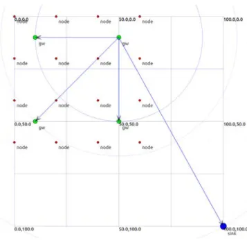
Lastly, the placements of nodes are distributed in square, rectangle, and circle and the area of them are nearly the same. The simulation time is 50 seconds to let all nodes become the cluster head one time. We create 50, 100 and 200 nodes in our experiments, and the first node is the sink. The only work of the sink is to receive packets and does not involve in the measurement generation or the cluster selection. The other nodes act as sensor node and form clusters.
As for the IoT scenario simulation, the measurement generation rate is the same as the cluster scenario simulation with both the periodic and Poisson pattern. The nodes are distributed as a grid with height and width 20 meters. The simulation lasts for 20 seconds because there is no clustering algorithm. There are one small scale simulation with 16 nodes and one large scale simulation with 64 nodes. Four gateways are located in the center of each square of sensor nodes. The sink lies far from the sensor nodes. The time constraint of measurements is assigned as constant at value 5 seconds.
Fig. 4-3 The disc distribution of nodes with radius 225.
Fig. 4-4 The square distribution of nodes with length 400.
Fig. 4-5 The square distribution of nodes with length 800 and width 200.
Fig. 4-6 The small IoT scenario distribution of nodes.
Fig. 4-7 The big IoT scenario distribution of nodes.
Chapter 5 Experimental results
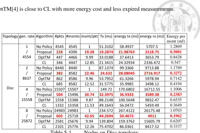
In this section, we compare the packet reception rate, the time of transmission state, the average number of measurements contained in one transmission, and the expired packets. The following tables are categorized by 3 topologies, 2 generation patterns. Each category has 2 tables, one for measurement arrival and energy consumption, while the other for measurement drop. As we can see, when the packet generation rate λ is low, our proposal tends to spend more transmission time and deliver less packets. The tables contain only the time of transmission because the time of reception and idle state have some relation with the time of transmission. Since the Wi-Fi connection is the ad-hoc mode, one node transmits, and all the other nodes receive. Therefore, the time of reception is roughly one hundred times of the time of transmission. The idle time occupies most of the timeline. There exist other states such as CCA_BUSY, SWITCHING, and SLEEP, but their time are too short to be counted. Thus, the idle time can be approximated by the total timeline minus the transmission time and the reception time.
A. Periodic measurement generation
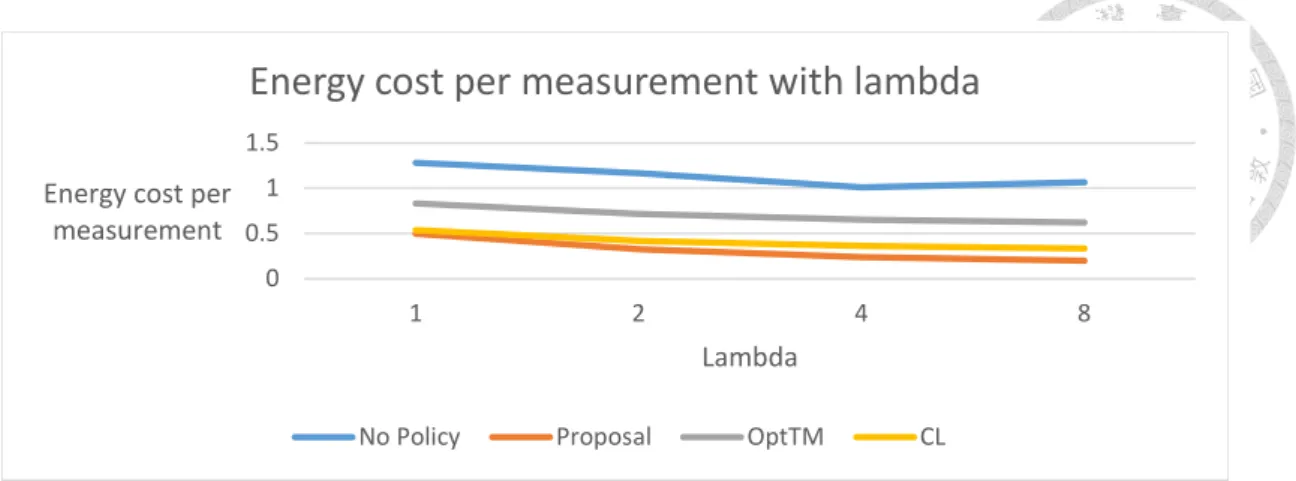
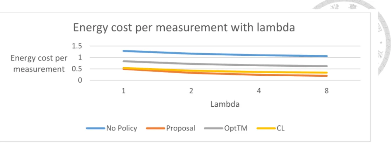
When the packet generation interval follows the periodic generation pattern, the aggregation policy can precisely predict the next moment at which the measurements arrive. This gives the data aggregation algorithms a test of energy saving. Our proposal has great advantage on energy saving over the counterparts with 50% lower than the result without data aggregation policy. While our proposal puts strong emphasis on energy saving, CL[7] strikes an elegant balance between energy and time constraint. CL delivers high amount of measurements with compact usage of packets. The performance of
OptTM[4] is close to CL with more energy cost and less expired measurements.
Topology gen. rate Algorithm #pkts #msmts msmt/pkt Tx (ms) energy tx (mJ) energy rx (mJ) Energy per msmt (mJ)
Disc 1 / 4554
No Policy 4545 4545 1 51.3102 58.4937 5707.5 1.2869 Proposal 228 4396 19.28 19.2874 21.98763 2118.75 0.5001 OptTM 447 4466 9.99 33.0188 37.6413 3653.79 0.8428 CL 346 4447 12.85 21.3415 24.32934 2336.472 0.547 2 /
8637
No Policy 8440 8440 1 87.1374 99.3366 9713.88 1.1769 Proposal 382 8582 22.46 24.632 28.08045 2716.917 0.3272 OptTM 862 8586 9.96 53.7952 61.3266 5978.94 0.7142 CL 685 8582 12.52 31.5775 35.9985 3498.12 0.4194 4 /
15558
No Policy 15507 15507 1 149.72 170.6802 16712.55 1.1006 Proposal 504 15496 30.74 32.3975 36.9333 3589.38 0.2383 OptTM 1558 15388 9.87 88.2148 100.5648 9832.47 0.6535 CL 1332 15358 11.53 49.1643 56.0472 5459.49 0.3649 8 /
25872
No Policy 24983 24983 1 234.572 267.4122 26175.48 1.0703 Proposal 603 25718 42.65 44.2694 50.4672 4911 0.1962 OptTM 2581 25676 9.94 139.804 159.3762 15605.79 0.6207 CL 2101 25776 12.26 75.4702 86.0361 8417.52 0.3337
Table 5-1. Nodes on Disc topology
Topology gen. Algorithm expired miss Drop
Disc 1 / 4554
No Policy 0 9 0.19%
Proposal 46 112 3.46%
OptTM 0 88 1.93%
CL 1 106 2.34%
2 / 8637
No Policy 0 197 2.28%
Proposal 13 42 0.63%
OptTM 0 51 0.59%
CL 0 55 0.63%
4 / 15558
No Policy 0 51 0.32%
Proposal 5 57 0.39%
OptTM 0 170 1.09%
CL 0 200 1.28%
8 / 25872
No Policy 0 889 3.43%
Proposal 13 141 0.59%
OptTM 0 196 0.75%
CL 0 96 0.37%
Table 5-2. Node drops on Disc topology
Fig. 5-1 Energy cost per measurement with lambda, Disc, periodic
0 0.5 1 1.5
1 2 4 8
Energy cost per measurement
Lambda
Energy cost per measurement with lambda
No policy Proposal OptTM CL
Topology gen. rate Algorithm #pkts #msmts msmt/pkt Tx (ms) energy tx (mJ) energy rx (mJ) Energy per msmt (mJ)
Square 1 / 4554
No Policy 4554 4554 1 51.1114 58.2669 5687.91 1.2794 Proposal 204 4445 21.78 19.3115 22.01508 2123.031 0.4952 OptTM 445 4503 10.11 32.8103 37.4037 3630.99 0.8306 CL 358 4490 12.54 21.1282 24.08616 2321.019 0.5364 2 /
8638
No Policy 8638 8638 1 88.1759 100.5204 9829.65 1.1636 Proposal 365 8583 23.51 24.44 27.86154 2697.711 0.3246 OptTM 854 8562 10.02 53.6372 61.1466 5969.19 0.7141 CL 683 8600 12.59 31.3957 35.7912 3482.04 0.4161 4 /
15560
No Policy 15495 15495 1 137.447 156.6897 15347.31 1.0112 Proposal 496 15505 31.26 32.1939 36.7011 3565.08 0.2367 OptTM 1543 15504 10.04 88.594 100.9971 9870.54 0.6514 CL 1320 15518 11.75 49.1792 56.0643 5473.26 0.3612 8 /
25874
No Policy 25280 25280 1 236.328 269.4138 26380.74 1.0657 Proposal 594 25806 43.44 44.4468 50.6694 4939.14 0.1963 OptTM 2562 25763 10.05 140.244 159.8778 15635.88 0.6205 CL 2026 25812 12.74 75.153 85.6743 8399.61 0.3319
Table 5-3. Nodes on Square topology
Topology gen. rate Algorithm expired miss Drop rate
Square 1 / 4554
No Policy 0 0 0%
Proposal 48 61 2.39%
OptTM 0 51 1.11%
CL 0 64 1.4%
2 / 8638
No Policy 0 0 0%
Proposal 10 45 0.63%
OptTM 0 76 0.87%
CL 0 38 0.43%
4 / 15560
No Policy 0 65 0.41%
Proposal 4 51 0.35%
OptTM 0 56 0.35%
CL 0 42 0.26%
8 / 25874
No Policy 0 594 2.29%
Proposal 12 56 0.26%
OptTM 0 111 0.42%
CL 0 62 0.23%
Table 5-4. Node drops on Square topology
Fig. 5-2 Energy cost per measurement with lambda, Square, periodic
0 0.5 1 1.5
1 2 4 8
Energy cost per measurement
Lambda
Energy cost per measurement with lambda
No Policy Proposal OptTM CL
Topology gen. rate Algorithm #pkts #msmts msmt/pkt Tx (ms) energy tx (mJ) energy rx (mJ) Energy per msmt (mJ)
Rectangle 1 / 4554
No Policy 4554 4554 1 51.378 58.5711 5713.29 1.2861 Proposal 222 4450 20.04 19.3992 22.11504 2119.656 0.4969 OptTM 445 4515 10.14 33.0903 37.7229 3665.37 0.8355 CL 355 4495 12.66 21.2233 24.19458 2343.087 0.5382 2 /
8638
No Policy 8611 8611 1 88.0342 100.359 9823.92 1.1654 Proposal 365 8592 23.53 24.5761 28.0167 2717.379 0.326
OptTM 854 8588 10.05 54.0358 61.6008 6014.85 0.7172 CL 669 8597 12.85 31.6097 36.0351 3503.94 0.4191 4 /
15560
No Policy 15493 15493 1 149.253 170.1486 16653 1.0982 Proposal 470 15483 32.94 32.2753 36.7938 3573.45 0.2376 OptTM 1543 15510 10.05 88.777 101.2059 9893.79 0.6525 CL 1298 15524 11.95 49.4885 56.4168 5496.45 0.3634 8 /
25874
No Policy 25710 25710 1 238.707 272.1261 26636.88 1.0584 Proposal 573 25793 45.01 44.269 50.4666 4922.1 0.1956 OptTM 2562 25743 10.04 140.12 159.7374 15618.33 0.6205 CL 1997 25791 12.91 75.0115 85.5132 8371.83 0.3315
Table 5-5. Nodes on Rectangle topology
Topology gen. rate Algorithm expired miss Drop rate
Rectangle 1 / 4554
No Policy 0 0 0%
Proposal 38 66 2.28%
OptTM 0 39 0.85%
CL 1 58 1.29%
2 / 8638
No Policy 0 27 0.31%
Proposal 5 41 0.53%
OptTM 0 50 0.57%
CL 0 41 0.47%
4 / 15560
No Policy 0 67 0.43%
Proposal 9 68 0.49%
OptTM 0 50 0.32%
CL 0 36 0.23%
8 / 25874
No Policy 0 164 0.63%
Proposal 13 68 0.31%
OptTM 0 131 0.5%
CL 0 83 0.32%
Table 5-6. Node drops on Rectangle topology
B. Poisson measurement generation
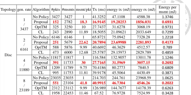
In contrast to the periodic measurement generation, Poisson measurement generation has different intervals between measurements' generation. This attribute of the Poisson measurement generation makes the aggregation policy hard to decide when the next measurements arrive. The aggregation policy would be tested with its robustness of delivering measurements in time. Our proposal depends heavily on predicting the arrival of the next measurements. Therefore, more packets are expired during the aggregation process. In some cases, our proposal drops about 20% of the total packets. CL also suffers from the changing time interval. The drop rate has its maximum at 15% while the measurements generate at the speed of one measurement per second. OptTM remains robust with little regards to how the time interval alters. The highest drop rate is about 5% and occurs when the measurement generation rate is one measurement per second.
Fig. 5-3 Energy cost per measurement with lambda, Rectangle, periodic
0 0.5 1 1.5
1 2 4 8
Energy cost per measurement
Lambda
Energy cost per measurement with lambda
No Policy Proposal OptTM CL
Topology gen. rate Algorithm #pkts #msmts msmt/pkt Tx (ms) energy tx (mJ) energy rx (mJ) Energy per msmt (mJ)
Disc 1
/ 3437
No Policy 3427 3427 1 41.3252 47.1108 4588.38 1.3746 Proposal 152 2782 18.3 16.9145 19.28253 1856.031 0.6931 OptTM 325 3250 10 27.7437 31.6278 3068.19 0.9731 CL 243 2890 11.89 18.5055 21.09621 2033.649 0.7299 2
/ 6161
No Policy 6146 6146 1 65.8721 75.0942 7328.28 1.2218 Proposal 251 5679 22.62 20.7894 23.69988 2281.893 0.4173 OptTM 588 5876 9.99 40.6692 46.3629 4512.57 0.789
CL 473 6000 12.68 25.5787 29.15973 2829.789 0.4859 4
/ 11880
No Policy 11817 11817 1 116.584 132.9057 13011.78 1.1246 Proposal 391 11733 30 27.7165 31.5969 3057.15 0.2692 OptTM 1209 11789 9.75 70.4186 80.2773 7840.5 0.6809 CL 995 11753 11.81 39.9178 45.5064 4430.49 0.3871 8
/ 23189
No Policy 23035 23035 1 214.703 244.761 23968.59 1.0625 Proposal 551 23104 41.8 40.9915 46.7304 4546.26 0.2022 OptTM 2312 23112 9.99 126.989 144.7677 14178.39 0.6263 CL 1958 22453 11.46 67.52 76.9728 7524.99 0.3428
Table 5-7. Nodes on Disc topology
Topology gen. rate Algorithm expired miss Drop rate
Disc 1
/ 3437
No Policy 0 10 0.29%
Proposal 454 201 19.05%
OptTM 74 113 5.44%
CL 260 287 15.91%
2 / 6161
No Policy 0 15 0.24%
Proposal 247 235 7.82%
OptTM 5 280 4.62%
CL 35 126 2.61%
4 / 11880
No Policy 0 63 0.53%
Proposal 57 90 1.23%
OptTM 0 91 0.76%
CL 0 127 1.06%
8 / 23189
No Policy 0 154 0.66%
Proposal 14 71 0.36%
OptTM 0 77 0.33%
CL 0 736 3.17%
Table 5-8. Node drops on Disc topology
Fig. 5-4 Energy cost per measurement with lambda, Disc, Poisson
0 0.5 1 1.5
1 2 4 8
Energy cost per measurement
Lambda
Energy cost per measurement with lambda
No policy Proposal OptTM CL
Topology gen. rate Algorithm #pkts #msmts msmt/pkt Tx (ms) energy tx (mJ) energy rx (mJ) Energy per msmt (mJ)
Square 1 / 3466
No Policy 3462 3462 1 41.3052 47.088 4584.87 1.3601 Proposal 151 2795 18.5 16.8823 19.24584 1854.708 0.6885 OptTM 337 3304 9.8 27.5443 31.4004 3046.11 0.9503 CL 263 3108 11.81 18.4356 21.01665 2026.215 0.6762 2
/ 6171
No Policy 6171 6171 1 66.1168 75.3732 7366.92 1.2214 Proposal 232 5604 24.15 20.8843 23.80809 2299.227 0.4248 OptTM 567 5858 10.33 40.9978 46.7376 4550.31 0.7978 CL 444 5862 13.2 25.4516 29.01483 2813.685 0.4949 4
/ 11875
No Policy 11828 11828 1 117.137 133.5363 13073.76 1.1289 Proposal 352 11721 33.29 27.4341 31.275 3042.63 0.2668 OptTM 1137 11781 10.36 70.5391 80.4147 7863.72 0.6825 CL 905 11718 12.94 39.867 45.4485 4427.88 0.3878 8
/ 23177
No Policy 22974 22974 1 196.533 224.0481 21949.05 0.9752 Proposal 539 23096 42.84 40.8768 46.5996 4550.31 0.2017 OptTM 2330 23135 9.92 126.939 144.7101 14169.18 0.6255 CL 1953 23013 11.78 68.5513 78.1485 7640.64 0.3395
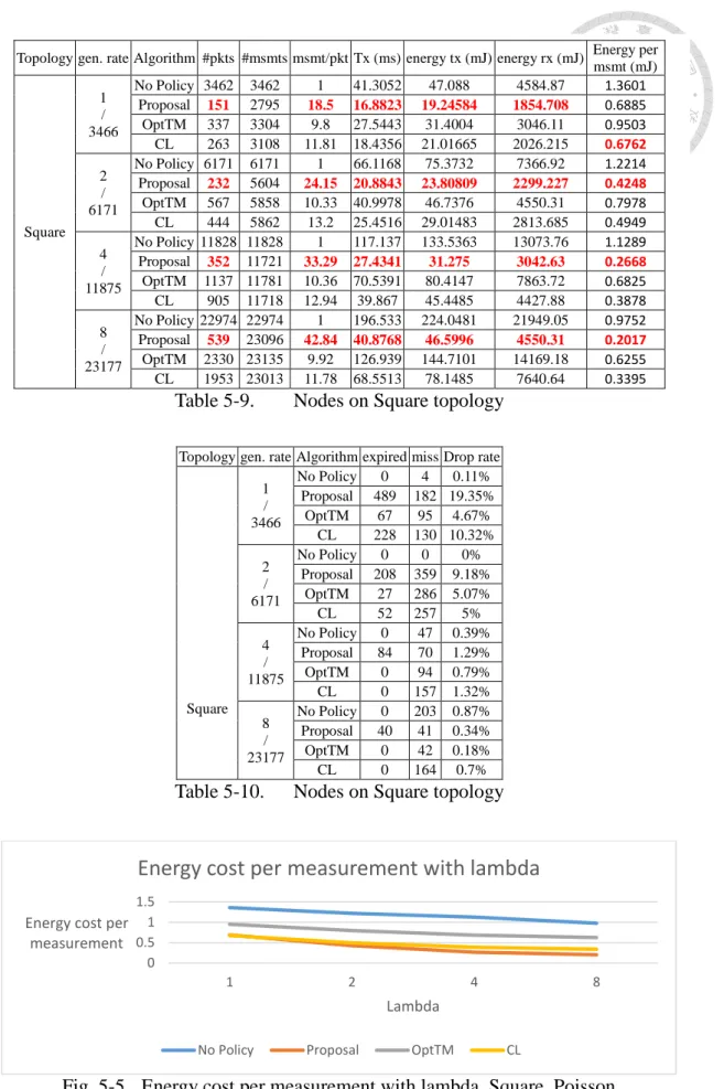
Table 5-9. Nodes on Square topology
Topology gen. rate Algorithm expired miss Drop rate
Square 1
/ 3466
No Policy 0 4 0.11%
Proposal 489 182 19.35%
OptTM 67 95 4.67%
CL 228 130 10.32%
2 / 6171
No Policy 0 0 0%
Proposal 208 359 9.18%
OptTM 27 286 5.07%
CL 52 257 5%
4 / 11875
No Policy 0 47 0.39%
Proposal 84 70 1.29%
OptTM 0 94 0.79%
CL 0 157 1.32%
8 / 23177
No Policy 0 203 0.87%
Proposal 40 41 0.34%
OptTM 0 42 0.18%
CL 0 164 0.7%
Table 5-10. Nodes on Square topology
Fig. 5-5 Energy cost per measurement with lambda, Square, Poisson
0 0.51 1.5
1 2 4 8
Energy cost per measurement
Lambda
Energy cost per measurement with lambda
No Policy Proposal OptTM CL
Topology gen. rate Algorithm #pkts #msmts msmt/pkt Tx (ms) energy tx (mJ) energy rx (mJ) Energy per msmt (mJ)
Rectangle 1 / 3466
No Policy 3466 3466 1 41.3504 47.1393 4590.45 1.36 Proposal 145 2941 20.28 17.0442 19.43037 1873.806 0.6606
OptTM 337 3300 9.79 27.8387 31.7361 3083.61 0.9617 CL 260 3082 11.85 18.3124 20.8761 2015.595 0.6773 2
/ 6171
No Policy 6164 6164 1 66.1182 75.3747 7364.46 1.2228 Proposal 232 5811 25.04 20.9457 23.87814 2310.222 0.4109 OptTM 567 6023 10.62 41.4944 47.3037 4602.84 0.7853 CL 439 6014 13.69 25.6223 29.20947 2833.125 0.4856 4
/ 11875
No Policy 11791 11791 1 117.288 133.7088 13090.83 1.1339 Proposal 360 11717 32.54 27.67 31.5438 3060.03 0.2692 OptTM 1137 11783 10.36 70.4997 80.3697 7854.51 0.682
CL 888 11789 13.27 40.182 45.8076 4472.58 0.3885 8
/ 23177
No Policy 22994 22994 1 215.373 245.5254 24038.1 1.0677 Proposal 527 23098 43.82 40.905 46.6317 4540.98 0.2018 OptTM 2330 23090 9.9 126.717 144.4572 14140.14 0.6256 CL 1919 23013 11.99 68.6482 78.2589 7647.39 0.34
Table 5-11. Nodes on Rectangle topology
Topology gen. rate Algorithm expired miss Drop rate
Rectangle 1 / 3466
No Policy 0 0 0%
Proposal 388 137 15.14%
OptTM 77 89 4.78%
CL 253 131 11.07%
2 / 6171
No Policy 0 7 0.11%
Proposal 159 201 5.83%
OptTM 5 143 2.39%
CL 14 143 2.54%
4 / 11875
No Policy 0 84 0.7%
Proposal 63 95 1.33%
OptTM 0 92 0.77%
CL 0 86 0.72%
8 / 23177
No Policy 0 183 0.78%
Proposal 20 59 0.34%
OptTM 0 87 0.37%
CL 0 164 0.7%
Table 5-12. Nodes on Rectangle topology
Fig. 5-6 Energy cost per measurement with lambda, Rectangle, Poisson
0 0.5 1 1.5
1 2 4 8
Energy cost per measurement
Lambda
Energy cost per measurement with lambda
No Policy Proposal OptTM CL
C. Topology
In our environment setting, topology affects the node distribution, and the node distribution is related to the cluster construction. For cluster heads, different cluster construction results in different number of incoming measurements. The experiment results show that no obvious relationship between the topologies.
D. Measurement generation rate (lambda)
While the topology has no obvious effect on our experiments, the measurement generation rate does have effect on energy cost and expiration rate. The higher generation rate, for all algorithms, the higher energy efficiency. The energy efficiency is defined as the energy cost per measurement. Aside with the energy cost, the expiration rate also drops with the increase of measurement generation rate. For our proposal, not only the energy efficiency is increased, but also the number of measurements per packet is increased, which means more measurements can be involved in the aggregation.
E. Scalability
Network environments often bring about a problem of scalability. With nodes scaling up from 50 to 200, the traffic load of the system also increases. With data aggregation applied to the system, the energy cost per measurement is decreased. While different number of nodes consists the network, we expect the change in the efficiency of the data aggregation. In the experimental result, however, we find that the energy saved by aggregation do not change much with the size of the network. Notice that when there are 200 nodes and no data aggregation policy is applied, the energy cost begins to rise while the lambda increases from 4 to 8.