動態對比增強磁共振影像參數之估測 : 位移效應之修正

國立臺灣大學工學院醫學工程學研究所 碩士論文

Graduate Institute of Biomedical Engineering College of Medicine and College of Engineering

National Taiwan University Master Thesis

動態對比增強磁共振影像參數之估測:位移效應之修正 Estimation of Dynamic Contrast Enhanced Magnetic Resonance Imaging Parameters : Motion Artifact Correction

許皓翔 Hao-Hsiang Hsu

指導教授：陳中明 博士 張允中 醫師 Advisor: Chung-Ming Chen, Ph.D.

Yeun-Chung Chang, M.D. Ph.D.

中華民國 97 年 7 月

July,2008

誌謝

首先，我要向指導教授台大醫工所 陳中明老師致上最高敬意與感謝。在研究 所的求學與研究過程中，在陳老師的引領與指導下，我才有機會可以接觸到這些 專業的領域並學習更多新的事物。陳老師治學嚴謹，成就卓越，並積極創新研究，

認真嚴謹的研究精神與精準確實的研究態度，都讓我受益良多。

另外，我還要特別感謝台大醫院放射科 張允中醫師，張醫師提供了這次研究 中最重要的數據與資料。並在過去的一年裡，在百忙之中還要抽空與我討論並一 起參與實際的研究過程，甚至在週末也常犧牲他的假期與我一同解析與研究數 據，由於他的協助與指導，讓我很快的增進有關醫學方面的知識。

在此一併感謝張醫師的助理雅琪小姐，在一些數據和報告上面也常幫我很多 忙，讓我可以免於奔波與整理。還要感謝在展書樓研究室的眾學長姐和學弟妹，

謝謝你們熱心的幫我解決一些研究上的小問題。並特別感謝在最後階段一直給我 勉勵的慧真學姐和基展學長以及一同奮戰到最後的劍威。

在此特別感謝台大電機所的郭立威學長，承蒙他多年來的幫助讓我有勇氣持 續面對各種艱困的挑戰，並得以完成我的夢想。

還要感謝秋芳，總是無怨無悔的陪伴與支持我的想法，是我在精神上的強力 支柱，讓我可以勇往直前的追尋夢想。

最後更要謝謝我親愛的家人。父親與母親在研究所時期全力的支持我的想法 並提供我無後顧之憂的資源，還有妹妹一直以來對家裡的幫忙，特別是到最後階 段真的讓我很感動。

研究所生涯看似很長，其實一溜煙就過去了。那些喜悅和艱澀的回憶也將更 豐富我的人生旅程，讓我更勇於面對未來的挑戰。

Albert 2008.08

ii

中文摘要

動態對比增強磁共振影像(DCE-MRI)為一應用快速 MRI 掃瞄序列觀測身體內 注射的對比劑進入血液中微灌流(perfusion)的情形。此應用對於觀察服用抗血管新 增藥物病患的治療與評估有很顯著的成果。而對比劑進入人體血液循環系統到達 腫瘤部位到代謝出來的行為模式往往可由不同的數學模型來描述。

目前有相當多的應用在於藉由量測這些數學模型的參數進而推得對比劑在循 環系統或腫瘤組織附近的流動情形。由這些流動的難易程度亦可以非侵入方式估 測腫瘤特性。

本研究的病人以肺癌病患為主，並施以 Avastin 抗癌藥物作為抗血管新增治療 藥物。希望可以透過動態對比增強磁共振影像(DCE-MRI)的特性，早期預測並評估 此抗癌藥物的化療效果。而本研究所採用的分析軟體 Mistar 可供我們選擇不同的 數學模型來進一步評估治療的效果。

不過此軟體受限於本身功能的限制，對於肺部切面影像在掃瞄中的呼吸等自 然位移與誤差未能進一步調整與修正。故本研究除了獲取動態對比增強磁共振影 像(DCE-MRI)的數學模型參數外，更進一步提出影像前處理的方式來修正因為移動 所造成的誤差影像。經過動態比對，修正後的影像有很明顯的改進。

除了影像位移的改進，另外我們也發現透過對於位移的校正，對這些動態對 比增強磁共振影像(DCE-MRI)的數學模型參數之分佈曲線有很顯著且明顯的影響。

因此位移效應之修正對於影像品質和參數之數值分佈有很重要的影響，我們希望 這些影響對於此抗癌藥物的化療效果有指標性的評估作用。

關鍵詞：動態動比增強磁共振影像、藥物動力學數學模型、影像處理、位移校正。

Abstract

Dynamic-contrast-enhanced MRI (DCE-MRI) is the usage of fast pulse sequence MRI for monitoring the perfusion of contrast materials in the blood stream. This application is useful in evaluating patients taking angiogenesis inhibitors. The behavior of the contrast material in the blood stream can then be modeled using a variety of different mathematical models.

Currently, by measuring select data and employing the different mathematical models, it is possible to estimate the flow characteristics of the contrast materials in the blood stream as well as around the tumor. Subsequently, by using the different flow characteristics, it is possible to evaluate the tumor in a non-invasive way.

The patients in this study were lung cancer patients, and had been given Avastin.

By employing DCE-MRI, it may be possible to predict and evaluate the effect of the chemotherapy early in the treatment course. This study employs Mistar, which is the software that provides the multitude of mathematical models for the evaluation treatment response.

Due to limitations of the software, however, inconsistencies resulting from image translation between tomography slices—due to spontaneous movements such as breathing—cannot be adjusted or corrected. Therefore, besides acquiring the DCE-MRI data for mathematical models, this study further employs image pre-processing for the correction of imaging errors due to subject movement. After dynamic comparison and correction, the image is vastly improved.

Besides improvements in image quality, translational correction also drastically improves the data used in the mathematical models. The usage of translational correction, therefore, greatly affects the final image quality, as well as the statistical

iv

distribution of the data being measured. We hope these changes will have a landmark impact on the final evaluation of the effectiveness of the angiogenesis inhibitors as well.

Keywords：Dynamic Contrast Enhancement Magnetic Resonance Imaging, Tofts Model,

Imaging processing, Motion Correction

Contents

論文口試委員審定書

誌謝 ………..i

中文摘要 ……….………ii

Abstract ……….………..iii

Contents …..……….……...v

Lists of figures ……….……….…...vii

List of Tables ……….………...x

Chapter 1 Introduction

1.1 Dynamic Contrast Enhanced Magnetic Resonance Imaging ………...1

1.2 Tumor Angiogenesis ……….3

1.3 Theory in DCE-MRI ……….5

1.4 Pharmacokinetic Model ………..12

1.5 Tofts Model ……….19

1.6 Application in DCE-MRI ………...24

Chapter 2 Theory in segmentation

2.1 Segmentation in normalized cuts method ……….………..29

2.2 Gradient Vector Flow ………..………...34

Chapter 3 Method

3.1 Clinical Experiment .………...38 3.2 Pre-processing in DICOM images .……..……….………..39 3.3 Mistar software processing ……..……….………..47

Chapter 4 Results

4.1 Results from Mistar software ……….……….……….50 4.2 Data Analysis ……….………...57

Chapter 5 Discussion

5.1 Problems in Data Analysis ……….………...63 5.2 Inaccuracy Problems ……….64

Chapter 6 Conclusion

6.1 Conclusion ..………….……….65 6.2 Future Work ……….……….67

Reference ………68

Lists of Figures

Figure 1.1 The phenomenon about tumor angiogenesis ………...3

Figure 1.2 (a) Signal intensity curve before bolus injection. (b) Contrast agent is diffusion to the interstitial space. (c) After the first pass of the bolus, the SI increases further until the concentration of the contrast agent in the blood and the interstitial space of the tissue are equal. (d) After this equilibrium phase, the contrast medium is progressively washed out from the interstitial space as the arterial concentration decreases. ………..………. ..6

Figure 1.3 Angiogenesis starts with cancerous tumour cells releasing molecules, angiogenic promoter substances that send signals to surrounding normal host tissue. The small gray circles indicate contrast agent molecules. The contrast agent is administered as a single intravenous bolus injection at point 2. The contrast agent leaks into the extravascular-extracellular space (EES), also called the leakage space, through VVOs and widened interendothelial junctions (line 2 to line 3). At first the contrast agent accumulates in the extravascular tissue before it diffuses back into the vasculature from which it is excreted (line 3 to line 4). In an MR image the accumulation and wash-out of contrast agent is observed as changes in the MR signal intensity which is proportional to the concentration of contrast media. The time- intensity curve to the left in the fi gure shows the intensity of the MR signal from the zoomed region before (line 1 to line2) and after injection of contrast agent (line 2 to line 4). ………10

Figure 1.4 Three compartments in tracer kinetic model ……….12

Figure 1.5 Illustration of General Kinetic Model ………...15

Figure 1.6 Illustration of Patlak Model ………..16

Figure 1.7 Illustration of Brix Model ………..………...18

Figure 1.8 Illustration of Tofts Model …..………..21 Figure 1.9 Contrast-enhanced magnetic resonance images (top row) and signal enhancement ratio (SER) parametric maps (bottom row), acquired before treatment (A), 2 weeks after the first cycle of doxorubicin-cyclophosphamide (B), and at the end of chemotherapy, before surgery (C), for a patient with locally advanced breast cancer.

Blue, green, and red color coding corresponds to low, moderate, and high values,

respectively. ………..………..25

Figure 1.10 Columns show anatomic subtraction images, corresponding Transfer constant maps, and histograms from pixel data. Row shows data before treatment and after one and two cycles of mitoxantrone and methotrexate chemotherapy, respectively ………...…..28

Figure 2.1 A case where minimum cut gives a bad partition ……….………....33

Figure 3.1 Image sequence in the clinical experiment ……….………..38

Figure 3.2 Reference and Temporal images ………...…39

Figure 3.3 Registration problem in sequential images. ……….……… 40

Figure 3.4 Adjust motion problem by moving temporal image to reference image …. 40 Figure 3.5 Select proper ROI in reference image. ………...……….. 41

Figure 3.6 Get proper ROI from the reference image to compare with the similar area in the temporal images ……….……….. 41

Figure 3.7 Contour which decided by user ……… 42

Figure 3.8 Make outside gray level be zero ………... 42

Figure 3.9 Prepare proper ROI for normalize cut ...……….. ……… 43

Figure 3.10 Results which determined by the normalize cut operation …….….…….. 43

Figure 3.11 Four maps (test image, edge map, edge map gradient, normalized GVF field for determined gradient vector flow ………..……….……44

Figure 3.12 Running gradient vector flow program to determined the contour ……….44 Figure 3.13 Final image which decided by normalize cut and gradient vector flow ….45

Figure 3.14 Correlation between reference and temporal image ……….….. 45 Figure 3.15 Shift temporal images to the arbitrarily position which correlation value is maximum ………...… 46 Figure 3.16 Interface in operating Mistar software ……….…….……. 47 Figure 3.17 Select processing area to in Mistar software. If we select large area, it will spend more time to finish the calculation. ………. 48 Figure 3.18 Processing the calculation (blue image is the area which selected to calculate) ………...………. 49 Figure 3.19 DCE-MRI parameter maps (upper right is v_e, upper left is k_ep, lower right is v_p, and lower left is k^trans) ………... 49 Figure 4.1 Select tumor contour by doctor to make sure the area is exactly in tumor position ………..……… 50 Figure 4.2 Four parameters maps results which calculated by Mistar software, the yellow line in the pictures are the tumor position and shape decided by doctor …..…. 51

Lists of Tables

Table 1.1 Three Standard Kinetic Parameters ………..……... 20

Table 1.2 Individual patient data showing tumour size, mean difference, coefficient of variation (CoV) and repeatability for K^trans and IAUC(60) for two scans …..….…….. 26

Table 4.1 Four parameter values in each patient include the mean and standard deviation ……… 53 ~ 56

Chapter 1 Introduction

1.1 Dynamic Contrast-Enhanced Magnetic Resonance Imaging

Dynamic contrast-enhanced magnetic resonance imaging (DCE-MRI) is a kind of MR images modality which over a period of time after the injection of contrast agent into vein. It’s about computer-enhanced modality that relies on a special algorithm and mathematic model to estimate blood flow.

The DCE-MRI technique is based on the continuous acquisition of 2D or 3D MR images during the distribution of an paramagnetic contrast agent bolus. The contrast agent is a gadolinium-(Gd) based which is able to enter the extravascular extracellular space (EES) via the capillary bed. The pharmacokinetics of Gd distribution are modeled by a 2- or multi-compartment model and has been shown to be a useful predictor of the biological response of angiogenesis [1]. Many different methods for image acquisition and data analysis have been described for use in DCE-MRI. The analysis models are designed to derive the optimal relevant components from the dynamic MR signal changes and to relate these to the underlying physiological processes which are taking place in the tissue.

In particular, the dynamic contrast enhanced MRI combined with physiological model-based analysis has been widely used in the study of tumor angiogenesis and in

the development and trial of anti-angiogenesis drugs. The derivation of physiological data from dynamic contrast MRI relies on the application of appropriate pharmacokinetic models to describe the distribution of contrast media following its systemic administration [2].

1.2 Tumor Angiogenesis

Angiogenesis is a physiological process involving the growth of new blood vessels from pre-existing vessels. It’s a normal process in growth and development, as well as in wound healing. However, this is also a fundamental step in the transition of tumors from a dormant state to a malignant state.

Fig 1.1 The phenomenon about tumor angiogenesis [3]

Tumor angiogenesis is the proliferation of a network of blood vessels that penetrates into cancerous growths (Fig 1.1), supplying nutrients and oxygen and removing waste products. Tumor angiogenesis actually starts with cancerous tumor cells releasing

molecules that send signals to surrounding normal host tissue. This signaling activates certain genes in the host tissue that, in turn, make proteins to encourage growth of new blood vessels [3]. The development of new blood vessels, is required for tumors to grow larger than 2-3 mm in size, and provided both nutrients and access to the systemic circulation with possible subsequent metastasis. This angiogenic process is mediated by several potent peptides, which include fibroblast growth factors and vascular endothelial growth factors [4].

Due to the characteristic in tumor angiogenesis, we can use the protocol of dynamic magnetic resonance imaging to measuring the tumor response indirectly.

1.3 Theory in DCE-MRI

Dynamic contrast-enhanced MRI is a method of physiological imaging, based on fast or ultra-fast imaging, with the possibility of following the early enhancement kinetics of a water-soluble contrast agent after intravenous bolus injection. This technique provides clinically useful information, by depicting tissue perfusion, capillary permeability, and composition of the interstitial space. The most important advantages of this technique are its abilities to monitor response to preoperative chemotherapy, identify areas of viable tumor before biopsy, and provide physiological information for improved tissue characterization and detection recurrent tumor tissue after therapy [5].

The extracellular distribution of fluid MR contrast agents is among blood plasma and the interstitial spaces. When a contrast agent is administered intravenously by a rapid bolus injection, it is first diluted in the blood of the peripheral vein and the right heart, before it passes through the lungs and the left heart into the peripheral circulation (Fig. 1.2a).

During first pass of the contrast agent through the capillaries, a fast diffusion occurs into the tissue, due to the high concentration gradient between the intravascular and the interstitial space: in normal tissues, approximately 50% of the circulating contrast agent diffuses from the blood into the extravascular compartment during the first pass.

Fig 1.2 (a) Signal intensity curve before bolus injection. (b) Contrast agent is diffusion to the interstitial space. (c) After the first pass of the bolus, the SI increases further until the concentration of the contrast agent in the blood and the interstitial space of the tissue are equal. (d) After this equilibrium phase, the contrast medium is progressively washed out from the interstitial space as the arterial concentration decreases. [5]

This first-pass diffusion is essentially different from that during the second pass and later. At this initial moment, there is no contrast agent in the interstitial space, and the agent has its highest possible plasma concentration, because it is diluted in only a very small part of the total plasma volume, namely that volume that enters into the right side of the heart at the same time as the bolus (Fig. 1.2b).After the first pass, the diffusion rate immediately drops, because the concentration of the re-circulating contrast medium has decreased owing to further dilution in the blood and partial accumulation in the

interstitial space throughout the body. The length of the time interval between the end of the first pass and the equilibrium state, with equal concentrations of contrast medium in plasma and interstitial space, depends on the size of the interstitial space (Fig. 1.2c).

After this equilibrium phase, the contrast medium is progressively washed out from the interstitial space as the arterial concentration decreases (Fig. 1.2d).

Only in highly vascular lesions with a small interstitial space does early washout occur within the first minutes after bolus injection. The aim of dynamic contrast enhance MRI is detect and depict differences in early intravascular and interstitial distribution as this process is influenced by pathological changes in tissues [5].

Numerous studies using dynamic contrast enhanced MRI have demonstrated that malignant tumors generally show faster and higher levels of enhancement than is seen in normal tissue. This enhancement characteristic reflects the features of the tumor microvasculature which in general will tend to demonstrate increased proportional vascular and higher endothelial permeability to the contrast molecule than do normal or less aggressive malignant tissues.

Cancer can develop in any tissue of the body that contains cells capable of division.

The earliest detectable malignant lesions, referred to as cancer are often a few milli- meter or less in diameter and at an early stage. In vascular tumors cellular nutrition depends on diffusion of nutrients and waste materials and places a severe limitation on

the size that such a tumor can achieve.

Conversion of a dormant tumor to a more rapidly growing invasive neoplasm, may take several years and is associated with visualization of the tumor. The development of neovascularization within a tumor results from a process known as angiogenesis.

These angiogenically competent cells have the ability to induce neovascularization through the release of angiogenic factors. There are positive and negative regulators of angiogenesis. Release of a promoter substance stimulates the endothelial cells of the existing vasculature close to the neoplasia to initiate the formation of solid endothelial sprouts that grow toward the solid tumor [2].

The following figure (Fig 1.3) illustrate the concept from tumor cell angiogenesis to the MRI signal intensity curve during the process of inject contrast agent. (a) Growth of a malignant tumor depends on its ability to stimulate neighboring vasculature to initiate formation of new blood vessels that can grow into the tumor and supply it with oxygen and nutrients. Angiogenesis starts with cancerous tumor cells releasing molecules, angiogenic promoter substances that send signals to surrounding normal host tissue.

These signals activate certain genes in the host tissue that, in turn, make proteins to encourage growth of new vessels. A new blood capillary can form by sprouting of endothelial cells from the wall of an existing small vessel. The cells at first form a solid sprout, which then hollows out to form a tube. This process continues until the sprout

encounters another vessel, with which it connects, allowing blood to circulate.

(b) The resolution of an MR image is determined by the field of view (FOV) and the matrix size. The pixel size and the thickness of the image slice give the volume of the voxel shown in the figure. One voxel contains many different cells even when using the smallest FOV and the largest matrix size possible. This means that the MR signal obtained from one voxel is the average of the proportion of tissue covered by the voxel.

(c) The zoomed region shows a cross section through a blood vessel and the surrounding extravascular tissue consisting of tumor cells, extracellular components and normal cells. The vessel wall is mainly made up of endothelial cells. The small grey circles indicate contrast agent molecules. The contrast agent is administered as a single intravenous bolus injection at point 2. The contrast agent leaks into the extravascular- extracellular space (EES), also called the leakage space (line 2 to line 3). How fast the contrast agent extravasates is determined by the permeability of the microvessels, their surface area, and the blood flow.

At first the contrast agent accumulates in the extravascular tissue before it diffuses back into the vasculature from which it is excreted. It usually by the kidneys, although some contrast media have significant hepatic excretion (line 3 to line 4). In an MR image the accumulation and wash-out of contrast agent is observed as changes in the MR signal intensity which is proportional to the concentration of contrast media.

Fig 1.3 Angiogenesis starts with cancerous tumour cells releasing molecules, angiogenic promoter substances that send signals to surrounding normal host tissue. The small gray circles indicate contrast agent molecules. The contrast agent is administered as a single intravenous bolus injection at point 2. The contrast agent leaks into the extravascular-extracellular space (EES), also called the leakage space, through VVOs and widened interendothelial junctions (line 2 to line 3). At first the contrast agent accumulates in the extravascular tissue before it diffuses back into the vasculature from which it is excreted (line 3 to line 4). In an MR image the accumulation and wash-out of contrast agent is observed as changes in the MR signal intensity which is proportional to the concentration of contrast media. The time- intensity curve to the left in the fi gure shows the intensity of the MR signal from the zoomed region before (line 1 to line2) and after injection of contrast agent (line 2 to line 4). [2]

The time-intensity curve to the left in the figure shows the intensity of the MR signal from the zoomed region before (line 1 to 2) and after injection of contrast agent (line 2 to line 4)

The mechanisms underlying the signal enhancement patterns seen on dynamic MRI include variations in regional blood flow, proportional blood vessel density, vascularization of existing blood vessels and variations in the surface area permeability of the endothelial membranes as well as the concentration difference which exists between plasma and the EES [2].

In many tumor types including breast, lung, prostate, and head and neck cancer, measurements of microvascular density made on histopathological samples correlate closely with clinical stage and act as an independent prognostic factor of considerable sensitivity. The rationale for this relationship appears to be that rapid tumor growth can be supported only in the presence of highly active angiogenesis and more aggressive tumor are therefore associated with increased evidence of angiogenesis-related microvasculature abnormalities. On the basis of this histopathological evidence it has been suggested that dynamic contrast enhanced MRI may also be able to provide independent indices of angiogenic activity and therefore act as a prognostic indicator in a broad range of tumour types [2].

1.4 Pharmacokinetic Model

When we want to attempt to quantify the observed contrast agent kinetics in terms of physiologically meaningful parameters we first need to define the elements of the tumor or tissue structure and the functional processes that affect the distribution of the tracer (the contrast agent). It is customary to represent tissue as comprising three or four compartments, each of which is a bulk tissue characteristic (we are unable to observe these compartments at their natural microscopic scale, but we can observe their aggregate effects at the image voxel scale or in a region of interest).

These compartments are the vascular plasma space, the extracellular extravascular space (EES), and the intracellular space (Fig. 1.4).

Fig 1.4 Three compartments in tracer kinetic model. [2]

All clinically utilized MRI contrast agents, and most experimental agents, are not pass into the intracellular space of the tissue due to their size, inertness, and non- lipophilicity, making the intracellular space un-probable using DCE-MRI; for this reason, the intracellular and other volumes are usually lumped together as a loosely defined intracellular space. According to fig 1.4 we can get the relationship between these compartments:

V_e+V_p+ =V_i 1 (1.1) V_p = −(1 Hct)V_b (

where

1.2)

Ve is the fractional EES, Vp is the fraction occupied by blood plasma, Vi is the

hanisms, that influence contrast agent dist

sses that accompany the faster growth rate of man

fraction occupied by the intracellular space, Vb is the fraction occupied by whole blood, and Hct is the haematocrit (typically about 0.4).

The functional parameters, or delivery mec

ribution in the intravascular space and the EES are usually assumed to be restricted to blood flow F and the endothelial permeability surface area product PS, which describe how leaky a capillary wall is.

There are two physiological proce

y tumors: an increased number of vessels and along with an increased permeability.

Therefore, one could expect an increased overall signal enhancement in the vicinity of tumors due to increasing vascular volume, vessel permeability, and increased flow.

ould des

ed semi quantitatively using parameters der

models were developed from Nuclear Medicine quantitative studi

.4.1 General Kinetic Model

el (GKM) is one approach to understanding the complex In the simplest model of tissue signal enhancement characteristics one c cribe 3 parameters: maximum signal enhancement, the rate at which this initial enhancement occurs“wash-in”, and the rate at which this increased signal decays

“wash-out”. However, it is important to consider this contrast dynamic with respect to the concentration of contrast agent in the vascular system as it perfusion the tissues. In simple graphical wash-in wash-out, it is assumed that the contrast agent immediately reaches equilibrium in the vascular system [6].

The data obtained with DCE-MRI is report

ived from pharmacokinetic models. Quantitative techniques that are often combined with rapid temporal sampling have been used together with simple pharmacokinetic models of tissues, obtaining parameters such as the transfer constant (K^trans), the rate constant (kep), and ve.

Most MRI kinetic

es but the limitations of MRI dictated specific modifications. A number of these MRI models are in current use, the primarily differentiated based on the way that they model the “arterial input function” (AIF).

1

The General Kinetic Mod

kinetics of contrast enhancement. The physiological processes of GKM are described in Figure 1.5, where the GKM simplifies the anatomy of the tumor into two functional components, the vascular space and the EES and one non-functional component, the intracellular space.

Vascular Space Vascular input function C

_p

(t)

Extra-vascular extra- cellular space (EES)

C

_t

(t)

K

^trans

K

_ep

Extra-vascular extra- cellular space (EES)

C

_t

(t) Vascular Space Vascular

input function C

_p

(t) K

^trans

K

_ep

Fig 1.5 Illustration of General Kinetic Model [6]

A contrast agent, spec weight agent which

rem

ifically a highly diffusible low molecular

ains extracellular, when introduced into the vascular space will leak into the EES at a characteristic rate and then will leak back into the vessel at another rate. Thus the net

change in concentration in the tumor can be described as:

trans t

p ep t

dC K C k C

dt

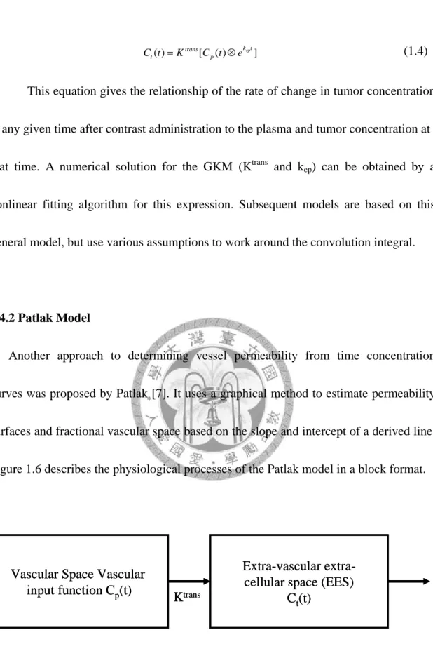
= − (1.3) where K^trans is a factor related to “wash in” and kep is a factor related to “wash-out” and the relationship between these parameters was the volume of extravascular-extracellular space ve. Furthermore, we can numerically evaluate these parameters for a variable concentration input function. This expression is mathematically described as a convolution integral.

(1.4)

relationship of the rat at any g

.4.2 Patlak Model

h to determining vessel permeability from time concentration cur

C t_t( )=K^trans[C t_p( )⊗e^{k tep} ]

This equation gives the e of change in tumor concentration iven time after contrast administration to the plasma and tumor concentration at that time. A numerical solution for the GKM (K^trans and kep) can be obtained by a nonlinear fitting algorithm for this expression. Subsequent models are based on this general model, but use various assumptions to work around the convolution integral.

1

Another approac

ves was proposed by Patlak [7]. It uses a graphical method to estimate permeability surfaces and fractional vascular space based on the slope and intercept of a derived line.

Figure 1.6 describes the physiological processes of the Patlak model in a block format.

Vascular Space Vascular input function C

_p

(t)

Extra-vascular extra- cellular space (EES)

C

_t

(t) K

^trans

Vascular Space Vascular input function C

_p

(t)

Extra-vascular extra- cellular space (EES)

C

_t

(t) K

^trans

Fig 1.6 Illustration of Patlak Model [7]

In this method, flow from the tissue space to the vascular space is assumed negligible and flow is assumed to be unidirectional. In this model, the contrast agent in

( ) ( )

trans t

p p p

K

∫

C τ τd v C t (1.5)

wher lasma volume. The term is sim e.

the tumor can be expressed as:

C t_t( )= +

0

e vp is the fractional p ilar in concept to the term v Dividing both sides of the equation by Cp(t) yields:

0^t _p( )

trans

t C d

C K τ τ v

=

∫

+

p

p p

C C (1.6)

The Patlak approach utilizes a simpler approach than the standard pharm mod

.4.3 Brix Model

is also a two compartment model in which the arterial input curve is assume

acokinetic el. A major advantage of the Patlak model is based in its incorporation of AIF.

However one limiting assumption of this model is that the contrast agent flows only into the tissue of interest. If the slope of the “Patlak” graph is not linear, then the assumption of no back flow is violated and the parameters generated would no longer be valid.

1

Brix model

d to be the result of a prolonged constant infusion that takes the shape of square wave (i.e. the contrast agent instantly reaches a plateau, remains constant for awhile and then instantly is over) which mixes in the vascular space and is slowly eliminated by renal excretion [8]. The input function is of magnitude Kin, the elimination constant is kel, and the rate constants describing the transfer of contrast agent from plasma to the

Central Compartment

Peripheral Compartment

K

_in

K

_el

K

₂₁

K

₁₂

Central Compartment

Peripheral Compartment

K

_in

K

_el

K

₂₁

K

₁₂

Fig 1.7 Illustration of Brix Model. [8]

The mathematical expression of the temporal response of SCM (t) / S0 is obtained:

^SCM_S^{( )t = +1 A v e}

{

^⎡⎣ ^{(k tel')−1⎤}⎦^{e(k tel)−u e⎡}⎣ ^{(k t21')−1⎤}⎦^{e(k t21)}

}

(1.7

0

)

W is the time–independent Gd-DTPA enhanced M s a

fitti

here SCM (t) RI signals, A i

ng parameter depending on the properties of the tissue of the sequence used, and of the infusion rate (Kin). Brix put forth a mathematical description that incorporated a term that allowed the adjustment of an AIF parameter.

.5 Tofts Model

es a different approach to the arterial input function (AIF), but reta

by diffusion transfer of contrast material between the vas

del to establish the time cou

to model the concentration of tracer with time. It con

1

Tofts model tak

ins the fundamental assumptions of the GKM (General Kinetic Model) [9],[10]. In the Tofts model, the input function is assumed to be the result of a pulse bolus injected into a two compartment system.

The arterial input is modified

cular space and body extravascular space; this system of compartments modifies the pulse bolus into a biexponential arterial input function [11].

This model consists of two parts: a compartmental mo

rse of the contrast agent (Gd-DTPA) tracer concentration in the tissue; and relate to observed MRI signal enhancement.

A compartmental model is used

sists of a plasma volume, connected to a large extracellular space which is distributed throughout most of the body (e.g., muscle). The kidneys drain tracer from the plasma, and hence from the extracellular space. We have modified this model by adding a fourth compartment, the lesion, which is connected to the plasma through a leaky membrane (Fig 1.8).

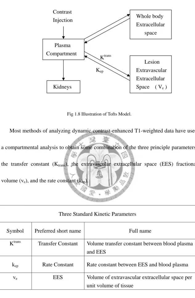
Fig 1.8 Illustration of Tofts Model.

Most methods of analyzin T1-weighted data have used a co

Three Standard Kinetic Parameters

Lesion Extravascular Extracellular Space ( V_e ) Kidneys

Whole body Extracellular

space Contrast

Injection

Plasma Compartment

K^trans Kep

g dynamic contrast-enhanced

mpartmental analysis to obtain some combination of the three principle parameters:

the transfer constant (Ktrans), the extravascular extracellular space (EES) fractional volume (ve), and the rate constant (kep).

Symbol Preferred short name Full name

K^trans Volume transfer constant between blood plasma

and EES Transfer Constant

kep Rate Constant Rate constant between EES and blood plasma ve EES Volume of extravascular extracellular space per

unit volume of tissue tandard Kinetic Param

Table 1.1 Three S eters.

Most methods of analyzing dynamic contrast-enhanced T1-weighted data have used a co

mpartmental analysis to obtain some combination of the three principle parameters:

the transfer constant (K^trans), the extravascular extracellular space (EES) fractional volume(ve), and the rate constant (kep). The transferconstant and the EES relate to the fundamental physiology, whereas the rate constant is the ratio of the transfer constant to

the EES [10]:

trans

ep e

K K

= v (1.8) rom the sh

data

h permeability, transfer constant is equal to the blood plasma flow per unit vol

The rate constant can be derived f ape of the tracer concentration vs time , whereas the transfer constant and EES require access to absolute values of tracer concentration. The transfer constant Ktrans has several physiologic interpretations, depending on the balance between capillary permeability and blood flow in the tissue of interest.

In hig

ume of tissue:

(1 )

trans

K =Fρ −Hct (1.9) Where F are Perfusion (or flow) of whole blood per unit mass o

the

racer flux is permeability (PS >> F)

f tissue,

ρ

means density of tissue, Hct represent for Hematocrit, P means total permeability of capillary wall, S means surface area per unit mass of tissue.

In the other limiting case of low permeability, where t

limited, the transfer constant is equal to the permeability surface area product between blood plasma and the EES, per unit volume of tissue [12]:

trans

K =PSρ (PS<<F) (1.10) Tracer flows passively from the blood pl eable capillary into the EES, thro

ate constant kep is formally the flux rate constant between the EES and blood plas

low-Limited Model (High Permeability)

con

d by setting the venous asma in a perm

ugh microscopic pores or defects in the capillary walls. It also called the interstitial space.

The r

ma. It’s always greater than the transfer constant K^trans. For a range of typical EES fractional volumes seen in tumors and multiple sclerosis (ve = 20% ~ 50%), kep is two to five times higher than K^trans [10].

F

Its first assumption is that arterial and venous blood have well-defined centrations, supplying and draining the tissue under study. Second, because permeability is high, venous blood leaves the tissue with a tracer concentration that is at all times in equilibrium with the tissue. Thus, soon after injection of the tracer, the arterial concentration is high, the venous concentration is low, and most of the tracer is being removed from the blood as it passes through the tissue.

For an extracellular tracer, the model can be extende

concentration equal to that of the EES. The effect of intravascular tracer on the MR signal can be ignored (ie, the vascular signal is small compared with the tissue signal).

In this case the following differential equation relating tissue concentration Ct to arterial

plasma concentration Cp can be obtained:

^dCt _{F (1}

dt = ρ − )( _P ^t)

e

Hct C C

−v (1.11)

S-Limited Model (Low Permeability)

considered as a single pool, with equal arte

bility surface area product of the cap

P

If flow is high, the blood plasma can be

rial and venous concentrations. The transport of tracer out of the vasculature is slow enough not to deplete the intravascular concentration.

The rate of uptake is then determined by the permea

illary wall and the difference between the blood plasma concentration and the EES concentration. If the contribution of tracer in the intravascular space is ignored, the

transport equation is

^t _{( P} ^t₎

e

dC C

PS C

dt = ρ − v (1.12)

.6 Application in DCE-MRI

netic resonance imaging (DCE-MRI) is being used in

be used as a biomarker, the method for quantifying the assay has to

n illustration of parametric analysis of DCE-MRI images using an emp

ng SER at each pix

g antiangiogenic trea

1

Dynamic contrast-enhanced mag

oncology as a noninvasive method for measuring properties of the tumor microvasculature.

For DCE-MRI to

be defined. There are several goals to be weighed in optimizing the biomarker definition. The biomarker needs to (1) maximize the sensitivity to biologic changes caused by treatment; (2) capture tumor heterogeneity, which is an important as a biomarker [13].

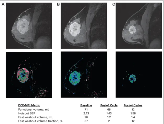
Fig 1.9 is a

irical parameter, the SER, for a patient with locally-advanced breast cancer treated with doxorubicin-cyclophosphamide (AC) chemotherapy. MRI was performed before chemotherapy, 2 weeks after the first cycle of chemotherapy, and at the end of AC treatment, before surgery, using a three–time point DCE-MRI method.

Pharmacokinetic properties of the tumor were quantified by computi

el, defined as SER＝(S1-S0)/(S2-S0), where S0, S1 and S2 are the pre-contrast (baseline), early post-contrast and late post-contrast signal intensities.

DCE-MRI is a promising biomarker candidate for assessin

tment. Correlative studies performed in combination with therapeutic trials have

demonstrated proof of concept for DCEMRI as a biomarker; however they have not been powered to adequately evaluate biomarker performance [13].

Fig 1.9 Contrast-enhanced magnetic resonance images (top row) and signal enhancement ratio (SER) parametric maps (bottom row), acquired before treatment (A), 2 weeks after the first cycle o

onstrates a single slice imaging technique. The image acquisition is p

f doxorubicin-cyclophosphamide (B), and at the end of chemotherapy, before surgery (C), for a patient with locally advanced breast cancer. Blue, green, and red color coding corresponds to low, moderate, and high values, respectively. [13]

Another paper dem

erformed in less than 500 ms making it relatively insensitive to respiratory motion.

Data from phantom studies and a reproducibility study in solid human tumor. The reproducibility study showed a coefficient of variation (CoV) of 19.1% for Ktrans and

or two commonly used parameters, K^trans and IAUC (60

improved to 16 and 13.9% if tumor of diameter less than 3 cm were excluded. The individual repeatability was 30.6% for K^trans and 26.5% for IAUC for tumor which are greater than 3 cm diameter [14].

The individual patient data f

), calculated from R1 values, are given in Table 1.2. Although no correlation was seen between T2 signal intensity and enhancement parameters, the second case in Table 1.2 had very high T2 compared with the other cases, consistent with a cystic nature of the metastasis. Guidelines from a recent US national cancer institute workshop on DCE–MRI state that tumors in a fixed superficial location should be at least 2 cm in diameter and other tumors should be at 3 cm in diameter. This study shows a tendency for greater variability with reducing size, and excluding lesions less that 3 cm in diameter reduced CoV.

Table 1.2 Individual patient data showing tumour size, mean difference, coefficient of variation (CoV) and repeatability for K^trans and IAUC(60) for two scans.[14]

and repeatability values (K^tra

benefits and show equ

g patients undergoing neo

al woman with a The colorectal liver metastases group also had lower CoV

ns 14.2 % and 26.5% and IAUC(60) 11 % and 21.3%, respectively), although this

may be related to the fact that this group had relatively larger tumor.

Another approach explore the randomized trials confirm these

ivalent survival for adjuvant and neo-adjuvant chemotherapy in patients with primary operable breast cancer [16-17]. A further benefit of neo-adjuvant chemotherapy is the opportunity to assess the chemo-responsiveness of the tumor. The overall response rates reported vary between 60% and 100%, with complete clinical responses ranging from 10% to almost 50%, avoiding mastectomy in most cases. Clinical responders have a better prognosis than do non-responders [18].

The prognostic importance of histo-pathologic response amon

-adjuvant chemotherapy for breast cancer is also recognized [19]. Patients who have complete pathologic response or pathologic minimal residual disease have a longer disease-free and overall survival compared with patients who have gross residual disease. The ability to identify non-responders early after the start of chemotherapy would be of major benefit because it would enable treatment to be adjusted or enable alternative and possibly more efficacious treatments, such as other types of chemotherapy or early surgery, to be offered as soon as possible [20].

Fig 1.10 shows the change in transfer constant in perimenopaus

gra

(middle row), an increase in the transfer constant med

de 3 infiltrating ductal carcinoma of the left breast not responding to mitoxantrone and methotrexate chemotherapy.

After one cycle of treatment

ian and range is seen (57% and 34%, respectively), compared with a 10% decrease in tumor size. After two treatments (bottom row), a further increase in the transfer constant median and range is seen (186% and 181%, respectively) on the transfer constant histogram, compared with a 11% increase in tumor size [21].

Fig 1.10 Columns show anatomic subtraction images, corresponding Transfer constant maps, and histograms from pixel data. Row shows data before treatment and after one and two cycles of mitoxantrone and methotrexate chemotherapy, respectively. [21]

Chapter 2 Theory in Segmentation

.1 Segmentation in normalized cuts method

a digital image into multiple reg

rpose algorithms and techniques have been developed for image seg

ed by Shi and Malik in 1997[23] . In this

2

Segmentation refers to the process of partitioning

ions. The goal of segmentation is to simplify or change the representation of an image into something that is more meaningful and easier to analyze [22]. Image segmentation is typically used to locate objects and boundaries (lines, curves, etc.) in images. The result of image segmentation is a set of regions that collectively cover the entire image, or a set of contours extracted from the image. Each of the pixel in a region are similar with respect to some characteristic or computed property, such as color, intensity, or texture.

Several general-pu

mentation. Since there is no general solution to the image segmentation problem, these techniques often have to be combined with domain knowledge in order to effectively solve an image segmentation problem.

The “normalized cuts” method was first propos

method, the image being segmented is modeled as a weighted undirected graph.

Each pixel is a node in the graph, and an edge is formed between every pair of pixels.

The weight of an edge is a measure of the similarity between the pixels. The image is

l dissimilarity between the diff

joint sets, A and B, by simply rem

w u v

=

partitioned into disjoint sets by removing the edges connecting the segments. The optimal partitioning of the graph is the one that minimizes the weights of the edges that were removed (the “cut”). Shi’s algorithm seeks to minimize the “normalized cut”, which is the ratio of the “cut” to all of the edges in the set.

The normalized cut criterion measures both the tota

erent groups as well as the total similarity within the groups. The grouping algorithm consists of the following steps:1. Given an image or image sequence, set up a weighted graph G = (V,E) and set the weight on the edge connecting two nodes to be a measure of the similarity between the two nodes. 2. Solve …(D-W)x = λDx for eigenvectors with the smallest eigenvalues. 3. Use the eigenvector with the second smallest eigenvalue to bipartition the graph. 4. Decide if the current partition should be subdivided and recursively repartition the segmented parts if necessary.

A graph G = (V,E) can be partitioned into two dis

oving edges connecting the two parts. The degree of dissimilarity between these two pieces can be computed as total weight of the edges that have been removed. In graph

theoretic language, it is called the cut :

cut A B)( ,

∑

( , ) (2.1)

e one that minimizes this cut value. Although there are an

The optimal of a graph is th

exponential number of such partitions, finding the minimum cut of a graph is a

d by recursively finding the minimum cuts that bise

cut criteria favo

well-studied problem and there exist efficient algorithms for solving it. Wu and Leahy [24] proposed a clustering method based on this minimum cut criterion. In particular, they seek to partition a graph into k-subgraphs such that the maximum

cut across the subgroups is minimized.

This problem can be efficiently solve

ct the existing segments. As shown in Wu and Leahy's work, this globally optimal criterion can be used to produce good segmentation on some of the images.

However, as Wu and Leahy also noticed in their work, the minimum

rs cutting small sets of isolated nodes in the graph. This is not surprising since the cut defined in (1) increases with the number of edges going across the two partitioned parts. Fig. 2.1 illustrates one such case.

Assuming the ance between the

two

Fig 2.1 A case where minimum cut gives a bad partition. [23]

edge weights are inversely proportional to the dist

nodes, we see the cut that partitions out node n1 or n2 will have a very small value.

aper pro

In fact, any cut that partitions out individual nodes on the right half will have smaller cut value than the cut that partitions the nodes into the left and right halves.

To avoid this unnatural bias for partitioning out small sets of points, the p pose a new measure of disassociation between two groups. Instead of looking at the value of total edge weight connecting the two partitions, our measure computes the cut cost as a fraction of the total edge connections to all the nodes in the graph. It’s call the

normalized cut (Ncut):

( , ) ^{( . ) ( , )} ( , ) ( , ) cut A B cut A B Ncut A B

assoc A V assoc B V

= + (2.2)

Where assoc(A,V) is the total connection from nodes in A and

r total normalized association within gro

to all nodes in the graph assoc(B,V) is similarly defined. With this definition of the disassociation between the groups, the cut that partitions out small isolated points will no longer have small Ncut value, since the cut value will almost certainly be a large percentage of the total connection from that small set to all other nodes.

In the same way, it can define a measure fo

ups for a given partition:

( , ) ^{( , ) ( , )} ( , ) ( , ) assoc A A assoc B B Nassoc A B

assoc A V assoc B V

= + (2.3)

and assoc(B,B) are total weights of wit

Where assoc(A,A) edges connecting nodes

hin A and B, respectively. We see again this is an unbiased measure, which reflects how tightly on average nodes within the group are connected to each other. Another

important property of this definition of association and disassociation of a partition is that they are naturally related:

( , ) ( . ) ( , )

( , ) cut A B cut Ncut A B

assoc A V assoc

= +

( , ) A B

B V

^{( , ) ( , ) ( , ) ( , )}

( , ) ( , )

assoc A V assoc A A assoc B V assoc B B

assoc A V assoc B V

− −

= +

( , ) ( , )

2 ( , ) ( , )

assoc A A assoc B B assoc A V assoc B V

= − +

2 ( , ) (2.4) Hence, the two partition

the

Nassoc A B

= −

criteria that we seek in our grouping algorithm, minimizing disassociation between the groups and maximizing the association within the groups , are in fact identical and can be satisfied simultaneously. In our algorithm, we will use this normalized cut as the partition criterion.

.2 Gradient Vector Flow

rs, are curves defined within an image domain that can mo

ugh the spatial domain of an image to min

2

Snakes [25], or active contou

ve under the influence of internal forces coming from within the curve itself and external forces computed from the image data. The internal and external forces are defined so that the snake will conform to an object boundary or other desired features within an image. Snakes are widely used in many applications, including edge detection , shape modeling [26-27], segmentation [28-29].

A traditional snake is a curve, that moves thro

imize the energy functional:

( ( ) )

1 '

0

1 (

2

2 '' 2

) ( ) _ext

E ^⎡α x s +β x s ^⎤⎥⎦+E x s ds (2.5) The external energy function Eext is derived from the its sma

=

∫

⎢⎣

image so that it takes on ller values at the features of interest, such as boundaries. Given a gray-level image I(x,y) , viewed as a function of continuous position variables (x,y), typical external energies designed to lead an active contour toward step edges are:

[ ]

(1) 2

( , ) ( , )

Eext x y = − ∇I x y

(2) 2

( , ) ( , ) ( , )

Eext x y = − ∇ G_σ x y ∗I x y

(2.6)

where G^σ(x,y)is a two-dimensional Gaussian function with standard deviation and gradient operator. If the image is a line drawing (black on white), then appropriate external energies include

ext

(2.7)

(3)

(4)

( , ) ( , )

( , ) ( , ) ( , )

ext

ext

E x y I x y

E x y G x y_σ I x y

=

= ∗

A snake that minimizes E must satisfy the Euler equation :

αx s^''( )−βx s^'''( )− ∇E =0 (2.8)

This can be viewed as a force balance equation

F_int+F_ext^{( )p} =0 (2.9)

The internal force discourages stretching and bending while the external potential force pulls the snake toward the desired image edges. The gradient vector flow snake approach is to use the force balance condition as a starting point for designing a snake.

It define below a new static external force field, which we call the gradient vector flow (GVF) field. To obtain the corresponding dynamic snake equation, we replace the potential force, yielding :

x s t_t( , )=αx s t^''( , )−βx s t^''''( , )+v (2.10) We call the parametric curve solving the above dynamic equation a GVF snake. It is solved numerically by discretization and iteration, in identical fashion to the traditional snake. Although the final configuration of a GVF snake will satisfy the force-balance equation, this equation does not, in general, represent the Euler equations of the energy minimization problem. This is because v(x,y) will not, in general, be an irrotational field . The loss of this optimality property, however, is well-compensated by the significantly improved performance of the GVF snake.

We define the gradient vector flow field V(x,y) = [u(x,y) , v(x,y)] to be the vector field that minimizes the energy functional

( ) ( )

( ) ( )

2 2

2

2 2

2

0 0

x x y

y x y

u u f f f

v v f f f

μ μ

∇ − − + =

∇ − − + = (2.11)

This variational formulation follows a standard principle, that of making the result smooth when there is no data. In particular, we see that when ∇ is small, the energy

f

is dominated by sum of the squares of the partial derivatives of the vector field, yielding a slowly varying field. On the other hand, when ∇ is large, the second term

f

dominates the integrand, and is minimized by setting v = ∇f . This produces the desired effect of keeping v nearly equal to the gradient of the edge map when it is large, but forcing the field to be slowly-varying in homogeneous regions.

The parameter μ is a regularization parameter governing the tradeoff between the first term and the second term in the integrand. This parameter should be set according to the amount of noise present in the image.

We note that the smoothing term —the first term within the integrand by Horn and Schunck in their classical formulation of optical flow [30]. It has recently been shown that this term corresponds to an equal penalty on the divergence and curl of the vector field [31]. Therefore, the vector field resulting from this minimization can be expected to be neither entirely irrotational nor entirely solenoidal.

Using the calculus of variations [32], it can be shown that the GVF field can be

found by solving the following Euler equations :

( ) ( )

( ) ( )

2 2

2

2 2

2

0 0

x x y

y x y

u u f f f

v v f f f

μ μ

∇ − − + =

∇ − − + = (2.12)

These equations provide further intuition behind the GVF formulation. We note that in a homogeneous region, the second term in each equation is zero because the gradient of f(x,y) is zero. Therefore, within such a region, and are each determined by Laplace’s equation, and the resulting GVF field is interpolated from the region’s boundary, reflecting a kind of competition among the boundary vectors [33].

Chapter 3 Method

3.1 Clinical Experiment

The image raw data is gathered by Dr.Chang in National Taiwan University Hospital.

This clinical experiment is performance in 1.5T Siemens MRI system. We use gadolinium as contrast agent and Avastin as the chemotherapy drugs.

After inject the contrast agent, we scan the patient’s lung 100 frames in about 100 seconds, each frame will have four sagittal view images and one axial view image.

t = 1 2 3 98 99 100

+

4 Sagittal lung images 1 axial lung image

Fig 3.1 Image sequence in the clinical experiment.

3.2 Pre-processing in DICOM images

After DCE-MRI experiments, the console will output DICOM format images. If we want avoid motion effect in Mistar software, we should do motion correct operation before the DICOM input to the Mistar software.

Suppose we have two images like figure 3.2. Left side is the reference image (we suppose the tumor position is correct ), and right side is temporal image ( the tumor position will have shift effect because of the motion during scan process ) which we want to correct it.

Reference Image Temporal Image

Figure 3.2 Reference image and temporal image.

The red circle indicate the tumor ( to simplify the motion problem, we assume the tumor volume in each image is the same with each other ), and we can clearly identify the tumor position (red circle) in reference image and temporal image is quite different. If we input the sequence DICOM image data to the Mistar software, we

Reference image

Temporal image 1

Temporal image 2

Temporal image 3

Temporal image 100

Figure 3.3 Registration problem in sequential images.

To solve this problem, we using correlation method in image registration. For example, if we have two images like figure 3.2. The goal is that we want to put tumor in both images in the same position (fig 3.4).

Figure 3.4 Adjust motion problem by moving temporal image to reference image.

In fact, we select reference image in first time. Then we will find out the proper ROI in reference image (Fig 3.5) making the correlation with temporal images.

Proper ROI

Fig 3.5 Select proper ROI in reference image.

We will get the proper ROI from the reference image to compare with the similar area in the temporal images (Fig 3.6)

Similar Area

ROI (Reference Image)

Temporal Image

Fig 3.6 Get proper ROI from the reference image to compare with the similar area in the temporal images.

To increase the specification in tumor property, we can select the tumor position by

contour by user (dot line) in Fig 3.7

By User defined

Step 1: Select the

Fig 3.7 Contour which decided by user.

tep 2: We set gray level in the area outside the contour be zero (black) in Fig 3.8 S

Fig 3.8 Make outside gray level be zero.

By automatic segmentatio

cut will do operation in Fig 3.9

n method

Step 1: Select the area which normalize

Fig 3.9 Prepare proper ROI for normalize cut.

Step 2: After running normalize cut program, we get a binary image and its corresponding gray level image in Fig 3.10.

Step 3: Run the gradient vector flow (GVF) program to determined the contour in Fig 3.11 ~ Fig 3.13

Fig 3.11 Four maps (test image, edge map, edge map gradient, normalized GVF field) for determined gradient vector flow.

Fig 3.12 Running gradient vector flow program to determined the contour

Fig 3.13 Final image which decided by normalize cut and gradient vector flow.

The similar area should be the possible area which tumor position is inside in the temporal images. Although the tumor position in temporal images is differ with each other, the tumor position in reference image will provide a standard to deal with the problem. Since we already get the ROI in both reference image and temporal image, the maximum correlation will determined the correct position.

After we do the correlation with the reference and temporal image, there exist many correlation coefficients. What we want is the maximum correlation coefficient.

The maximum correlation coefficient represent the most proper tumor position in the temporal images. Once we find the proper position, the next step is to shift the temporal images to the new position (fig3.8).

Fig 3.15 Shift temporal images to the arbitrarily position which correlation value is maximum.

Since we suppose the tumor is rigid, the reference image will change to get the most similarity in tumor shape. That is, the image which was corrected will be the next reference image. Under the assumption, we suppose to correct total temporal images in the whole image sequences.

software Mistar to accomplish the DCE-MRI study and entify the difference between image data with motion correct or not.

After we lunch the DICOM data from MRI console, it shows the lung image in both gittal and axial view in the upper right during the software window. In order to find e arterial input function (AIF), we select the axial view and set the ROI ( yellow uare ) in the aorta to get the AIF. The upper right shows the 100 time frames signal

.

3.3 Mistar software processing

We use the commercial id

sa th sq

intensity in aorta which used to be the AIF

Besides select the AIF, we also decided the area which need to be calculated in the software. The selection of the area should be include the tumor and not exceed to much to waste the processing time (fig 3.17).

Fig 3.17 Select processing area to in Mistar software. If we select large area, it will spend more time to finish the calculation.

When we decided the curve of AIF and the region which needed to be execute, then we can push the processing button to run the entire calculation like fig 3.18.