用於群聚多重轉態延遲錯誤的診斷解析度改善技術

(1)

國立臺灣大學電機資訊學院電子工程學研究所碩士論文

Graduate Institute of Electronics Engineering College of Electrical Engineering and Computer Science

National Taiwan University Master Thesis

用於群聚多重轉態延遲錯誤的診斷解析度改善技術 Diagnosis Resolution Improving Technique for Clustered

Multiple Transition Delay Faults 游彥勝

Yan-Shen You

指導教授：李建模博士 Advisor: Dr. Chien-Mo Li

中華民國 108 年 10 月

October 2019

(2)

誌謝

兩年多的碩士生活一下就過去了，卻學到了很多，也感謝所有人讓我能夠順利畢業。首先，要感謝我的指導教授，李建模教授，剛進碩班時，對於碩士生活的步調很不習慣，表現不好，但是老師從來都沒有生氣過，讓我很感動。也是老師激勵了我，

讓我認真面對之後的碩士生活。還要感謝我的父母與阿姨，阿姨提供我房間住，讓我不用承擔房租壓力；父母幫我支付生活雜費，減輕經濟的壓力。

再來要感謝學長們，柏瑋、彥鈞、恆毅、家誠、凱傑在我碩一時提供的修課、研究上的協助，尤其是同為診斷組的柏瑋學長，不厭其煩地教導我診斷領域的知識，非常謝謝；彥鈞、恆毅在我碩零實習時，聯發科的各種建議，讓我可以提前準備進入碩一；凱傑實驗室工作交接時，都幫助我很多；家誠在我研究或作業有困難時，也給我很多幫助。接著要感謝跟我同年的明庭、旻彥、采婕，你們在我研究、修課與心態上，

都讓我學習很多。接著要感謝學弟們，治硯、宜展、辰鋐、世棠與彥庭，首先謝謝同組的治硯，在我寫 paper 與論文時，經常跟我討論怎麼寫符合邏輯；接著謝謝你們常常聽我講很多研究上的困難，常常陪我到很晚才回家，讓我不至於寂寞，有人可以聊天與討論論文；謝謝宜展、彥庭 MSOC 期末 carry 我。

還要感謝在健身房遇到的所有人，健身是我在研究所生活裡，感到有興趣有動力去做的事情，也是我幾乎每天都會去的地方，跟朋友們聊天，能為一天充滿電，讓我去面對研究的苦悶，由衷感謝你們。

最後，再次由衷感謝，在碩士期間對我好的人們，真的很幸運遇到你們。

(3)

摘要

電源電壓干擾引起的電壓壓降造成轉態延遲錯誤群聚在一個小區域裡。之前針對

群聚多重轉態延遲錯誤的診斷工具獲得了好的準確率但差的解析度。這篇論文提出一

個改善針對群聚多重轉態延遲錯誤診斷工具解析度的技術。我們假設會看到很多回報

的嫌疑閘實體上聚集在真實嫌疑閘附近，我們的技術基於這個假設來刪除散落的嫌疑

閘。我們首先利用診斷分數抽取重要嫌疑閘。我們使用相關係數來決定最佳群集數，

使我們可以用K-means 演算法來為嫌疑閘分群。最後，我們刪除較不可能的嫌疑閘，

但保留重要的嫌疑閘。在基準電路上的模擬顯示了我們技術的能力。診斷工具加上我

們的技術解析度(0.35)比同樣的診斷工具沒有我們的技術(0.25)還要好，改善了 40.0%；

代價是我們的技術使得原本的準確度(0.83)下降了 0.03，損失了 3.6%。

關鍵字: 群聚多重錯誤、多重錯誤診斷、轉態延遲錯誤診斷

(4)

Abstract

Power supply noise induced IR drop can cause transition delay faults (TDF) clustered

in a small region. A previous diagnosis technique aiming at clustered multiple TDF

obtains good accuracy but bad resolution [Chen 18]. This thesis proposes a technique to

improve resolution of the diagnosis tool aiming at clustered multiple TDF. We assume

many suspects physically cluster around true suspects, so our technique prunes suspects

based on this assumption. We first extract important suspects by the diagnosis score.

Second, we use correlation coefficient to determine the optimal number of clusters so we can

apply the clustering algorithm to group suspects. Finally, we prune the least possible

suspects but keep important suspects. Simulation on benchmark circuits show the

effectiveness of our technique. Diagnosis resolution of the diagnosis tool with our

technique (0.35) is better than that of the same diagnosis tool without our technique (0.25),

which is improved by 40.0%. The cost is that our technique causes accuracy drops 0.03

from the original accuracy (0.83), which is dropped by 3.6%

Keyword:clustered multiple faults, multiple faults diagnosis, TDF diagnosis

(5)

List of Figures

Figure 1.1 IR-drop map of a real chip [Fang 18]... 2

Figure 1.2 Accuracy of clustered vs. random TDF (Commercial tool) ... 3

Figure 1.3 Accuracy of [Chen 18] and a commercial tool... 4

Figure 1.4 Resolution of [Chen 18] and a commercial tool ... 4

Figure 1.5 Suspects’ physical location ... 6

Figure 1.6 Accuracy of clustered random TDF ... 7

Figure 1.7 Resolution of clustered TDF ... 7

Figure 2.1 The evaluation graph of Figure 1.5 ... 13

Figure 2.2 Overall flow of [Chen 18] ... 15

Figure 2.3 Fanout recovergence problem of traditional critical path tracing [Chen 18] ... 17

Figure 2.4 Fanout recovergence problem of star tracing for TDF [Chen 18] ... 17

Figure 2.5 Example of star tracing for TDF (a) the first iteration (b) the second iteration (c) star tracing for TDF result ... 18

Figure 2.6 Overall flow of the K-means algorithm ... 21

Figure 2.7 Apply K-means algorithm to our experimental circuits (K=3) ... 22

Figure 3.1 Overall flow of our technique ... 24

Figure 3.2 Flow of determining the optimal number of clusters ... 25

Figure 3.3 The pseudo code of the block highlighted in Figure 3.2 ... 27

Figure 3.4 Pseudo of modified approximate covering heuristic ... 28

Figure 3.5 (a) Example without important suspects (b) Example with important suspects . 33 Figure 4.1 Accuracy of clustered TDF ... 37

Figure 4.2 resolution of clustered TDF ... 38

Figure 4.3 Accuracy at different levels of cluster density ... 39

Figure 4.4 Resolution at different levels of cluster density ... 39

Figure 4.5 Accuracy of W/IS and WO/IS ... 40

(7)

List of Tables

Table 3.1 Example of modified approximate covering heuristic (First iteration) ... 30

Table 3.2 Example of modified approximate covering heuristic (Second iteration) ... 31

Table 4.1 Circuit and pattern information ... 34

Table 4.2 Experimental results of α and β setting ... 36

Table 4.3 Runtime results ... 41

(8)

Chapter 1 Introduction

Chapter 1 gives brief introduction related to this thesis. Section 1.1 describes the

motivation of this thesis. Section 1.2 describes the proposed technique. Section 1.3

describes the contribution of our thesis. Section 1.4 describes the assumption made in this

thesis. Section 1.5 gives organization of this thesis.

1.1 Motivation

Delay sensitivity of cells to power supply noise increases as technology advances.

According to previous research, 10 % voltage drop in 180 nm process design increases 8%

propagation delay of gates [Saxena 03]. 10% voltage drop in 130 nm process design

increases 30% delay of gates [Krstic 01]. 1% voltage drop in 90 nm process design

increases 4% delay of gates [Tirumurti 04]. Power supply noise induces IR-drop when

large current flows through the resistive network [Ma 09]. Figure 1.1 shows an IR-drop

map of a real chip [Fang 18]. Typically, high IR-drop gates tend to cluster in local regions

which are highlighted with white circles (called IR-drop hot spot). Therefore, physically

clustered multiple TDF are more frequent than they used to be.

(9)

Figure 1.1 IR-drop map of a real chip [Fang 18]

When multiple TDF clustered in a small region, fault masking and fault reinforcement

effects can occur [Ye 14]. Fault masking means that a fault effect is blocked by other

faults. Fault reinforcement means that a fault is excited or a fault effect is propagated with

the help of other faults. As the TDF density gets higher, it is more difficult for diagnosis

tools to diagnose.

We define five terminologies used in this thesis. Suspects mean faults reported by

diagnosis tools. Culprits mean TDF that we injected into circuits for our fault simulation.

True suspects mean the suspects that we diagnosed correctly (injected in the circuit). False

suspects mean the suspects that we diagnose incorrectly (not injected). In this thesis, the

result of clustered multiple TDF is obtained by the average of three levels of density:

(10)

nearest, thousandth and hundredth. Levels of density are defined in Section 4.1.

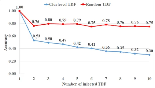
Current commercial diagnosis tools cannot diagnose clustered multiple TDF

accurately. Fig. 1.2 shows the average accuracy of four benchmark circuits when a

commercial tool diagnoses uniform TDF (red curve) and clustered TDF (blue curve).

Accuracy is the number of correctly diagnosed suspects over the number of injected

culprits. Accuracy of clustered TDF is worse than that of uniform TDF. We need a

diagnosis tool for clustered multiple TDF.

Figure 1.2 Accuracy of clustered vs. random TDF (Commercial tool)

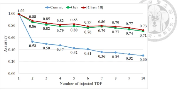
Chen proposes a diagnosis tool for clustered multiple TDF that obtains better accuracy

[Chen 18]. On the contrary, it obtains almost similar resolution as the commercial tool.

Accuracy and resolution are two diagnosis metrics which are used to evaluate the diagnosis

(11)

number of total diagnosed suspects. They range from zero to one. Higher accuracy and

resolution mean better diagnosis performance. Figure 1.3 and Figure 1.4 are obtained by

average accuracy and resolution of four benchmark circuits when diagnosis tools diagnose

clustered multiple TDF. The horizontal bar is the number of injected culprits. The

vertical bar is corresponding diagnosis metrics.

Figure 1.3 Accuracy of [Chen 18] and a commercial tool

Figure 1.4 Resolution of [Chen 18] and a commercial tool

(12)

Figure 1.3 shows [Chen 18] obtains much higher accuracy than the commercial tool

when multiple culprits injected to benchmark circuits. Figure 1.4 shows [Chen 18]

obtains almost similar resolution as the commercial tool. Although [Chen 18] identifies

more true suspects than the commercial tool, it chooses too many suspects to report. We

will introduce proposed techniques in [Chen 18] in Section 2.3. In this thesis, we want to

improve resolution obtained by [Chen 18]. When the diagnosis tool diagnoses clustered

multiple TDF, we will see many suspects cluster together around true suspects. If we

identify the optimal number of clusters of suspects, we can prune those smaller clusters

because they are less likely to be true suspects than larger clusters.

1.2 Proposed Technique

In this thesis, we propose a technique to improve resolution of diagnosis results.

First, we use correlation coefficient to determine the optimal number of clusters. Second,

we apply the K-means algorithm with the optimal number of clusters specified [Forgy 65]

to cluster suspects. Third, we extract important suspects by the diagnosis score. Finally,

we prune the least possible suspects but keep important suspects

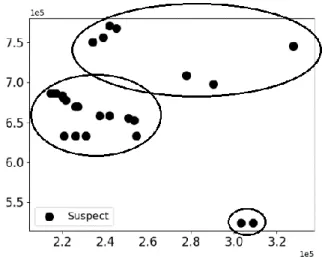
Figure 1.5 plots suspects’ physical location of a diagnosis result. We use this figure

to show what does our technique do. We determine the optimal number of clusters=3.

(13)

16,7 and 2 suspects in the largest, medium, and the smallest clusters, respectively.

Suspects in the black circle are in the same cluster. Then, we remove those clusters which

are smaller than a certain ratio (β) of the largest cluster. Where β is a user-specified

parameter, ranging from zero to one. In this diagnosis result, our technique prunes the

medium and the smallest cluster.

Figure 1.5 Suspects’ physical location

1.3 Contributions

We propose a technique for improving diagnosis resolution of clustered multiple TDF.

Figure 1.6 and Figure 1.7 show accuracy and resolution of the commercial tool (Comm.),

[Chen 18], and [Chen 18]+our technique (Our) when diagnosing clustered multiple TDF.

(14)

Figure 1.6 Accuracy of clustered random TDF

Figure 1.7 Resolution of clustered TDF

Figure 1.6 shows accuracy of our technique is almost as good as that of [Chen 18] only, and

much better than that of the commercial tool. This shows our technique keeps many true suspects. Figure 1.7 shows resolution of our technique is the best among three diagnosis

tools. Compared with [Chen 18] only, our technique obtains much better resolution. This

(15)

shows our technique effectively removes false suspects. The key contributions of this thesis

are summarized as follows.

 We consider physical information to improve resolution of clustered multiple TDF.

 We propose a heuristic to prune smaller clusters.

 To keep true suspects, we extract important suspects.

1.4 Assumptions

We make three assumptions in this thesis. First, we use transition delay fault as our

fault model. Transition delay fault is an abstract fault model that modeling delay-induced

culprits in the circuit. If a signal has a transition delay fault, its time frame two value is

stuck at 0 (slow to rise, transition from 0 to 1) or stuck at 1 (slow to fall, transition from 1

to 0). In this thesis, we assume clustered multiple culprits are caused by IR-drop, so they

are delay-related culprits. Transition delay fault is suitable for our assumption, so we use

it as our fault model.

Second, we assume many suspects are physically clustered together around true suspects when diagnosing clustered multiple TDF. In many cases, [Chen 18] reports many

suspects near true suspects. It is because their propagation paths are similar, faulty

responses are likely to be similar. Although this assumption is correct in most cases, there

(16)

are still incorrect in some cases. In other words, we may sometimes prune true suspects

which is in removed clusters.

Third, we assume circuits failed by a single IR-drop hot spot. In our experiments,

culprits are injected in a single cluster. There may be more than one IR-drop hot spot in

failing circuits, so this assumption is sometimes unrealistic. We made this assumption

because we want to simplify clustered multiple TDF issue. In the future, we can conduct

the other technique to handle clustered multiple TDF in multiple cluster.

1.5 Organization

The rest of the thesis is organized as follows. Chapter 2 reviews past research and

background knowledge. Chapter 3 presents the proposed technique. Chapter 4 shows

experimental results of the proposed technique. Chapter 5 discuss some issue in this

thesis and tips to improve the technique. Chapter 6 concludes this thesis.

(17)

Chapter 2 Background

Chapter 2 reviews background knowledge related to this thesis. Section 2.1

summarizes past research about multiple fault diagnosis. Section 2.2 summarizes past

research about clustered multiple fault diagnosis. Section 2.3 summarizes past research

about determining the optimal number of clusters. Section 2.4 introduces the diagnosis

tool used in our experiment. Section 2.5 gives brief introduction about the K-means

algorithm, which is used in our technique.

2.1 Prior Work in Multiple Fault Diagnosis

Multiple faults diagnosis is a difficult problem because simulation of many fault

combination is unrealistic for diagnosis. Many researchers tried to diagnose multiple

culprits by single fault simulation. Huisman used single location at a time (SLAT) patterns

which are failing patterns can be explained by a single fault. The algorithm found the

minimum suspects’ faulty response covering of SLAT patterns [Huisman 04]. This

method converts multiple faults diagnosis to single fault diagnosis. However, there are not

enough SLAT patterns for diagnosis. Wang proposed N-perfect algorithm and failing

output partition algorithm [Wang 06]. N-perfect algorithm iteratively selected one

suspects to explain part of failing patterns. It continued until all failing patterns are

(18)

explained or no suspects can explain remained failing patterns. When there was no

suspect can explain remained failing patterns, failing output partition algorithm partitioned

circuits to search suspects that partially explain failing patterns. The above research

cannot handle fault masking and fault reinforcement effect.

Ye proposed a graph-based diagnosis method [Ye 10]. He constructed fault-tuple

equivalence tree (FTET) for every failing patterns to find fault combination that cause the

faulty response. Fault-tuple contains the information of faulty location and faulty value.

Then, he scored fault-tuples in each FTET. Finally, he found suspects based on the score.

The fault masking and fault reinforcement are handled while choosing suspects in each

iteration. Chao proposed a technique to separate easy-to-detect faults and hard-to-detect

faults [Chao 14]. He separates the fail log into several parts and perform diagnosis

individually. Finally, He combines suspects reported by each diagnosis. This technique

obtains good accuracy, but resolution is relatively bad. [Chao 14] cannot handle fault

masking and fault reinforcement effect. All of above-mentioned research did not consider

physical information in the diagnosis.

Lee proposed a physical-aware diagnosis for multiple faults [Lee 17]. This technique

considers physical information of circuit under diagnosis (CUD). This technique takes

(19)

section as suspect unit. A section is a piece of interconnect, driven by a via. Suspect unit is

a basic unit to perform fault simulation to get simulation failures of it. Because this

technique has more detailed suspect unit, it obtains more accurate fault dictionary than other

traditional technique. Experimental results show that this technique obtains good accuracy

and resolution. Five pieces of research do not aim at clustered multiple TDF.

2.2 Prior Work in Clustered Multiple Fault Diagnosis

Pomeranz proposed a simulation-based method to diagnose clustered multiple TDF [12].

First, all suspects in the fault list were single-fault simulated. Most likely faults were paired

and double-faults simulated. Then, she ranked suspects based on the simulated response.

Accuracy of this technique is low. Runtime of this technique will increase nonlinearly

because of double faults simulation when there are many suspects in the suspect list. Lim

proposes a new scoring method which identifies faults that are dominated by other

clustered faults to rank suspects [Lim 12]. Experimental result shows that it obtains more

accuracy and less resolution than [Pomeranz 11].

2.3 Prior Work in Determining the Optimal Number of Clusters

Determining optimal number of clusters of suspects is one of tasks in our technique.

(20)

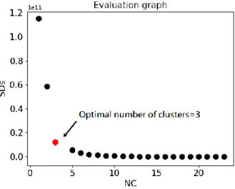
We use the evaluation graph to determine optimal number of clusters. The evaluation graph

is a two-dimensional plot. Figure 2.1 shows the evaluation graph of Figure 1.5. X-axis is

the number of clusters, ranging from 1 to the number of suspects reported by the diagnosis

tool. Y-axis is sum of squared distances of suspects to their cluster center (SDs), which is

the measurement of the K-means algorithm.

Figure 2.1 The evaluation graph of Figure 1.5

We review two pieces of research aiming at determining optimal number of clusters

from the evaluation graph. Salvador separates the point set of the evaluation graph into

two part to find knee point [Salvador 04]. He iteratively sets knee point from the second

point to the second-last point. In each iteration, he finds two best-fit lines of two point

sets, which are left and right side of knee point. He chooses the iteration that it results in

(21)

chosen iteration. Zhao uses the number of clusters vs. Bayesian information criterion

(BIC) graph [Zhao 08]. He proposes an algorithm to consider local information and

global information in the graph to find knee point. Local information uses successive

difference of previous, current and afterward values to see local changes. Global

information calculates angle of chosen successive three points to see global trend. His

algorithm considers global information, so it is more robust to find optimal number of

clusters than other methods which only consider local information. Both of them are not

suitable for our technique because they tend to find the point with the maximum curvature.

Moreover, both researches cannot determine knee point as one.

2.4 Diagnosis Tool [Chen 18]

In this paper, the diagnosis tool used for experiments is [Chen 18]. Figure 2.2

illustrate the overall flow of this technique. First, he performed star tracing for TDF for

every failing pattern to identify the potential suspects and generate initial fault list.

Second, he used single fault simulation for all the suspects in initial fault list to get

simulation failures. Finally, the approximate covering heuristic was conducted to select a

group of suspects by the diagnosis score.

(22)

START

Next Failing pattern?

Star tracing for TDF (Sec III A)

Single TDF simulation

Approximate covering heuristic(Sec III B)

Report candidates Yes

No

Figure 2.2 Overall flow of [Chen 18]

2.4.1 Star Tracing for TDF

Star tracing for TDF is motivated from [Akers 90], which is a backtracing technique to

reduce the number of faults needed to be considered during ATPG. Chen modify star

tracing for TDF to backtrace from failing outputs to find potential suspects. Because TDF

needs two time frames patterns to detect, star tracing for TDF backtraces time frame two

value. Star tracing for TDF backtraces the CUD based on four rules.

1. Star tracing for TDF marks failing output as star wires, and only backtraces star wires.

2. If the gate’s inputs are all non-controlling value, the algorithm marks all of them as

star wires and backtraces from these pins.

(23)

3. If at least one input of a gate is controlling value, the algorithm randomly marks one of

the input with controlling value as star wire and backtraces from this pin.

4. If there is a fanout stem, it is marked as star wire if at least one of its branch is star

wire.

Star tracing for TDF needs many iterations to identify potential suspects due to rule

three. When assignment of star wires has finished for all the iteration under a failing

pattern, star tracing for TDF updates the set of star wires by the function S*=∩S^*i. Where

S* is the set of star wires of the failing pattern. S^*i is the set of star wires in ith iteration.

We check if members in S* are activated, i.e., a star wire should have opposite value on

time frame one and time frame two. If a star wire is not activated, it is removed from S*.

When all failing patterns are backtraced, Initial fault list is generated by the union of S* of

each failing pattern

Star tracing for TDF handles fanout reconvergence problem. Take Figure 2.3 and

Figure 2.4 as example [Chen 18]. Values shown on these graphs are time frame two value,

and the sign a/b represents good value/faulty value. The fault effect of W1 stuck at 0 is

detected at primary output. Traditional critical path tracing stops at the and gate because

both inputs of the and gate is critical value. Nevertheless, star tracing for TDF randomly

(24)

choose an input in this condition. This difference results in star tracing for TDF adds W1

to the fault list, but traditional critical path tracing technique do not.

1

1 1 0

0/1 1

0/1

0/1 W₁/0

W₁/0 is detected W2

W3

1

1 1 0

0/1 1

0

0 CPT misses W₁

W2

W3

W₁

Figure 2.3 Fanout recovergence problem of traditional critical path tracing [Chen 18]

1

1 1 0

0/1 1

0/1

0/1 W₁/0

W₁/0 is detected W2

W3

1

1 1 0

0/1 1

0

0 Non-CPT finds W₁

W2

W3

W₁

*

* *

x x x

Figure 2.4 Fanout recovergence problem of star tracing for TDF [Chen 18]

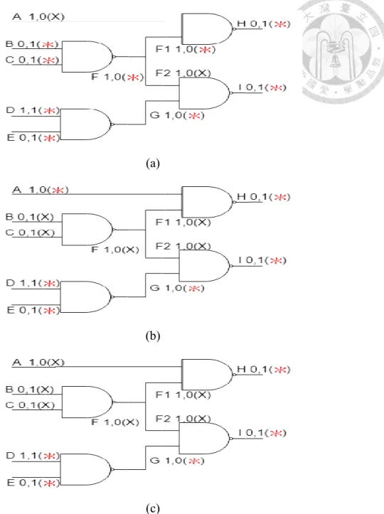
Figure 2.5(a)~(c) shows an example of star tracing for TDF. Under the same failing

pattern, Figure 2.5(a) and (b) shows different assignments of star wires. Because of rule 3,

star tracing for TDF randomly chooses a wire as star wire while it backtraces {A, F1} and

{F2, G}. Figure 2.5(c) shows the result by combining the assignment of (a) and (b) by the

function S*= S^*1∩S^*2. The initial fault list is {D,E,G,H,I} in this example. If we chooses

F2 as star wire in the Figure 2.5(a), the initial fault list could be {H,I}. This shows that if

we set more iteration, we get the more precise result.

(25)

(a)

(b)

(c)

Figure 2.5 Example of star tracing for TDF (a) the first iteration (b) the second iteration (c) star tracing for TDF result

2.4.2 Approximate Covering Heuristic

Unlike traditional greedy covering algorithm, which selects only one suspect in each

(26)

iteration, approximate covering heuristic selects a group of suspects so that fault masking

and fault reinforcement are likely to be tolerated. In our technique, we modify the

approximate covering heuristic. We extract important suspect which is suspects with the

highest diagnosis score in each iteration. The pseudo code of the modified approximate

covering heuristic is described in Section 3.3.

We define six terminologies used to explain how the approximate covering heuristic

works. TF is the union of failing output pins of all failing patterns obtained from

automatic test equipment (ATE). TP is the union of passing output pins of all failing

patterns obtained from ATE. SF is the union of all failing output pins of all failing

patterns obtained by single fault simulation. SP is the union of all passing output pins of

all failing patterns obtained by single fault simulation. UnCoveredTF is the set of TF that

have not been covered by selected suspects’ SF. The diagnosis score is the measurement

of suspects, which is used to measure the likelihood of suspects to be true suspects.

Approximate covering heuristic defines the size of UnCoveredTF∩SF (|unCoveredTF

∩SF|) as the diagnosis score, and it calculates diagnosis score for each suspect. In each

iteration, approximate covering heuristic finds suspects with the highest score. Then, it set

a threshold score, which is 90 percent of the highest score. Suspects with the score higher

(27)

than the threshold score is selected as final suspects. Fault masking and fault

reinforcement effect increase or decrease the diagnosis score, so it distorts the diagnosis

score. That means false suspects obtained the diagnosis score higher than true suspects

may occur. Approximate covering heuristic tolerate such condition by selecting suspects

with the second-to-best score.

Fault masking forces TFSF turn into TPSF, so the diagnosis score decreases. Fault

reinforcement forces TPSP turn into TFSP. The culprit influenced by fault reinforcement

effect generates a TF, but it generates SP under single fault simulation. Its diagnosis score

is not changed. On the contrary, the diagnosis score of suspects which can cover this TF

increase.

2.5 The K-means Algorithm

In our technique, we consider physical information to improve diagnosis resolution.

We apply the K-means algorithm to cluster suspects based on their physical location. The

K-means algorithm was proposed in 1965 [Forgy 65]. Although there are many clustering

algorithms over past fifty years, the K-means algorithm is still widely used due to its

simplicity and effectiveness [Jain 09].

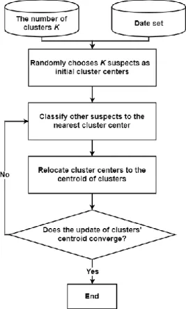
Figure 2.6 illustrates overall flow of the K-means algorithm. First, user specifies the

(28)

number of clusters K. Second, the algorithm randomly chooses K suspects as initial

cluster centers. Third, other suspects are classified to the nearest cluster centers such that

sum of squared distance of each suspect to their corresponding cluster center (SDs) is

minimum. Finally, cluster centers are relocated to the centroid of clusters. The algorithm

repeats the third step and the last step until update of cluster centers converge.

Figure 2.6 Overall flow of the K-means algorithm

Figure 2.7 demonstrate how we apply the K-means algorithm on experimental circuits.

The plot with the title “Suspects” shows the same suspect distribution as Figure 1.5, and we

(29)

use it as the data set to run the K-means algorithm. The plot with the title “initial” shows

the initialization of the K-means algorithm. The rest plots show the update of cluster

centers in each iteration. Their title is the number of iteration. From plot with the title “1”

to plot with the title “6”, we only show the legend of cluster centers, and rest markers are

suspects. Suspects with the same shape and the same color mean they are in the same

cluster. In this example, we specify the number of clusters K=3. Initially, the K-means

algorithm randomly chooses 3 cluster centers as shown in the plot with the title “initial”.

From the first update to the fifth update, we see cluster centers do not converge. The

update of cluster centers converges at the sixth update, so the K-means algorithm finishes.

Figure 2.7 Apply K-means algorithm to our experimental circuits (K=3)

(30)

Chapter 3 Proposed Technique

In this chapter, we introduce the proposed technique to improve the diagnosis result.

The organization of this chapter is as follows. Section 3.1 describes the overall flow of

our technique. Section 3.2 describes the method we determine the optimal number of

clusters. Section 3.3 describes the technique of important suspects extraction. Section

3.4 describes the method of suspect pruning.

3.1 Overall Flow

Figure 3.1 illustrates the overall flow of our technique. We parse the design

exchange format (DEF) file to obtain the gate coordinate of suspects. The DEF file

describes the information related to physical information, such as die size, physical location

of cells and macros of a chip. We determine the optimal number of clusters of suspects.

Then, we use the K-means algorithm with the optimal number of clusters. We extract

important suspects based on the diagnosis score during approximate covering heuristic.

Finally, we prune the least possible suspects but keep important suspects.

(31)

Figure 3.1 Overall flow of our technique

3.2 Determining the Optimal Number of Clusters

Many suspects cluster together around true suspects when diagnosing clustered

multiple TDF. To improve diagnosis resolution, we can prune smaller clusters. We

want adjacent suspects in the same cluster. Among many clustering algorithm, The

K-means algorithm is simple and suitable for our goal. Adjacent suspects will be in the

same cluster after the K-means algorithm. The K-means algorithm needs to specify the

optimal number of clusters, so we need a method to determine it.

Figure 3.2 illustrates the flow of determining the optimal number of clusters. Initially,

(32)

clusters=n), we calculate sum of squared distance of each suspect to their corresponding

cluster center (SDs) and record it. Then, we increase n by 1. We iteratively increase n until

it is larger than the number of suspects. After the loop terminates, an evaluation graph is

generated.

Figure 3.2 Flow of determining the optimal number of clusters

The evaluation graph is a two-dimensional plot. The x-axis is the number of clusters,

ranging from 1 to the number of suspects. The y-axis is SDs. Then, we use the correlation

coefficient (r) to determine the optimal number of clusters by the information in the

evaluation graph. r is defined by the following equation:

𝑟 = ∑^𝑛_𝑖=1(𝑥_𝑖 − 𝑚_𝑥)(𝑦_𝑖 − 𝑚_𝑦)

√∑^𝑛_𝑖=1(𝑥_𝑖− 𝑚_𝑥)²∑^𝑛_𝑘=1(𝑦_𝑖 − 𝑚_𝑦)²

(33)

where mx is the mean of vector x. my is the mean of vector y. xi and yi are the ith x, y

coordinate of the evaluation graph, respectively. Large r means two sets x and y are

highly correlated.

From Figure 2.1, the leftmost point of the evaluation graph is the highest because SDs

of every suspect to the only one cluster center is high. As the number of clusters increases,

SDs decreases. When the number of clusters is higher than the optimal number of clusters,

SDs changes slightly because redundant cluster centers only divide a cluster into two

clusters. This condition will not change SDs much. Based on this concept, we define the

optimal number of clusters as the first point that r of this point to the last point is higher

than a threshold (α).

Figure 3.3 illustrates the pseudo code of the block highlighted in Figure 3.2. Given a

list of points P in the evaluation graph. Line 1 refine size of P to 9 because too many points

will change the optimal number of clusters we obtain. Line 2 iterates index K from 1 to the

size of P. We calculate r of the Kth point to the last point of P in line 3. From line 4 to 8, if

r is larger than a threshold (α), K is determined as the optimal number of clusters and the loop

terminates. If r is not larger than α, the loop continues. After the loop terminates, we return

the optimal number of clusters. In this algorithm, the optimal number of clusters must be

(34)

defined because r of the last two points is 1.

Algorithm Determining the optimal number of clusters Input: Evaluation graph

Output: the optimal number of clusters

01 Refine P.size() to 9 02 for K=1 to P.size():

03 r = correlation coefficient of Kth point to the end of P 04 if r > α:

05 the optimal number of clusters = K 06 break

07 else:

08 continue

09 return the optimal number of clusters

Figure 3.3 The pseudo code of the block highlighted in Figure 3.2

We take Figure 2.1 as an example of determining optimal number of clusters. In this example, we set α to 0.8. First, we consider the first nine points. r of the first point to

the ninth point of P is 0.76, so we increase K by one. r of the second point to the ninth

point of P is 0.79, so we increase K by one again. When K=3, r is larger than α (0.8), so

we determine the optimal number of clusters=3.

3.3 Important Suspect Extraction

We extract important suspects which do not be removed during suspect pruning. We

modify the approximate covering heuristic to identify suspects with the highest diagnosis

score in each iteration as important suspects. Suspects with the highest score in a certain

(35)

iteration are the most likely to be true suspects among all suspects, so we identify them as

important suspects.

Figure 3.4 shows the pseudo code of modified approximate covering heuristic. This

figure shows how approximate covering heuristic works and how we extract important

suspects. We initialize unCoveredTF as TF, IS as empty set and iteration index i as 0 in

line 1. Where unCoveredTF is the set of failing output pins that have not been covered

and IS is the set of important suspects.

Algorithm Modified approximate covering heuristic Input SF of each suspect, TF of each suspect, fault list S

Output Final suspects (FS), important suspects (IS)

1 unCoveredTF = TF, IS = ø, i=0 2 while |unCoveredTF| > 0 3 SFⁱ=ø, Sⁱ=ø 4 Find sh and Scoreh

5 for s in S

6 If Scores > Scoreh×0.9 7 Sⁱ=Sⁱ∪s, SFⁱ=SFⁱ∪SFs

8 If Scoreh=0 or |Sⁱ| > 30

9 break

10 unCoveredTF = unCoveredTF - SFⁱ, S=S - Sⁱ 11 FS=FS∪Sⁱ, IS=IS∪sh

12 i=i+1 13 return FS, IS

Figure 3.4 Pseudo of modified approximate covering heuristic

From line 2 to line 15, a while loop continues until there is no uncovered failing output

(36)

pins in unCoveredTF. In line 3, we initialize the set of simulation failures of all suspects

selected in the ith iteration (SFi) and suspects selected in the ith iteration (Si) as the empty

set. In line 4, we find the suspect (sh) with the highest score (Scoreh). From line 5 to line

7, we select the suspect s whose score is higher than Scoreh×0.9. If a suspect s is selected,

Si takes the union of s and SFi takes the union of SFs. Where SFs is simulation failures of

s.

In line 8 to 9, we terminate the loop when one of two conditions is met: (1) Scoreh=0

or (2) the number of suspects selected in one iteration is larger than 30. The first

condition means suspects cannot cover any remaining test failure. The second condition

means we select many suspects to cover a few test failures. Selecting many suspects to

cover a few test failures results in poor resolution and cannot improve accuracy, so we

restrict the number of suspects selected in one iteration to 30. In line 10, we update

unCoveredTF and fault list S for the next iteration. In line 11, the set of final suspects (FS)

takes the union of Si and IS takes the union of sh. In line 12, we add 1 to i. After the loop

terminates, we return FS and IS.

In our experiments, we identified 16,539 true suspects as important suspects among

23,898 important suspects in 4.8 thousand diagnosis results. That means 69.20%

(37)

important suspects are true suspects. In Section 3.4, we demonstrate an example to show

the effect of extracting important suspects.

Table 3.1 and Table 3.2 show an example of the modified approximate covering

heuristic. FP is failing patterns. Op.k is the kth output under the pth pattern. “╳” means

the corresponding output pin is a failing output pin. SFsn is simulation failures of nth

suspect. We initialize unCoveredTF as TF, which is {O1.1, O1.2, O1.3, O2.1, O2.2, O2.3,

O2.4…O2.10} and the size is 13. Where O2.4…O2.10 means outputs O2.4 to O2.10, so the size

of TF is 7.

Table 3.1 shows the first iteration, the suspect with the highest score is s3 and the

highest score is 12, so we add s3 to IS. We choose a group of suspects S¹= {s1, s3} because

their score is larger than 12×0.9. Then, the covered TF={O1.1, O1.3, O2.1, O2.2, O2.3,

O2.4…O2.10} is removed from unCoveredTF. The remaining unCoveredTF is {O1.2}.

Table 3.1 Example of modified approximate covering heuristic (First iteration)

FP FP1 FP2

Score Output O1,1 O1,2 O1,3 O1,4…O1,10 O2,1 O2,2 O2,3 O2,4…O2,10

TF ╳ ╳ ╳ ╳ ╳ ╳ ╳ -

SFs1 ╳ ╳ ╳ ╳ ╳ 11

SFs2 ╳ ╳ 8

SFs3 ╳ ╳ ╳ ╳ ╳ ╳ 12

SFs4 ╳ ╳ 8

(38)

with the highest score is s4 and the highest score is 1, so we add s4 to IS. s2’s score is

smaller than 1×0.9, so it is not selected. We choose suspect S²={s4} in this iteration.

The remaining unCoveredTF is ø, so the modified approximate covering heuristic finishes.

Finally, we return IS={s3, s4}, and FS is S¹∩S² = {s1, s3, s4 }.

Table 3.2 Example of modified approximate covering heuristic (Second iteration)

FP FP1

Score Output O1,2 O1,4…O1,10

TF ╳ -

SFs2 0

SFs4 ╳ 1

3.4 Suspect Pruning

For reducing resolution of diagnosis results, we propose suspect pruning. We assume

clustered multiple TDF are caused by IR-drop, so suspects are physically clustered together

around true suspects. Based on this assumption, we can remove those smaller clusters

which are less likely to be our target culprits. If we have only one cluster, then there is

nothing we can do, so suspect pruning finishes. Otherwise, we remove those clusters

which are smaller than a certain ratio (β) of the largest cluster. β is a user defined

parameter, ranging from 0 to 1. Although we assume circuits failed by a single IR-drop

hot spot, we may remain multiple clusters during suspect pruning. We do not know which

(39)

Figure 3.5(a) and Figure 3.5(b) show the physical locations of suspects to demonstrate

the effectiveness of important suspect and suspect pruning. These are the same example

as Figure 1.6. Figure 3.5(a) is the result after suspect pruning without important suspects.

Figure 3.5(b) is the result after suspect pruning with important suspects. Black markers

are important suspects that remain after suspect pruning. Gray markers are non- important

suspects that remains after suspect pruning. Light gray markers are pruned suspects. We

add a slash to those markers to highlight it is pruned. Star markers are true suspects while

dot markers are false culprits. Figure 3.5(a) does not contain any black marker because

we do not extract important suspects. There are totally 23 suspects in these figures.

We continue the same example from Section 3.2, where the optimal number of clusters

=3. Figure 3.5(a) and Figure 3.5(b) show the result of this example. Suspects in the

black circle belong to the same cluster. There are 16, 7, 2 suspects in the largest, middle,

and the smallest clusters, respectively. We set β to 0.6 in this example. Because

16×0.6=9.6, so we prune suspects in the middle cluster (7 suspects) and the smallest cluster

(2 suspects). Figure 3.5(a) shows that if we do not consider important suspects, we would

prune nine suspects. Two of them are true suspects. Figure 3.5(b) shows the same

example but we keep six important suspects: four of them are true suspects, two of them

(40)

are false suspects. The legend IS represents important suspects. This example shows

that accuracy improves with important suspects. The cost is that we remain one false

suspect so the resolution degrades. Overall, we keep 19 suspects (6 are true suspects, 13

are false culprits) and prune 6 false suspects.

(a) (b)

Figure 3.5 (a) Example without important suspects (b) Example with important suspects

(41)

Chapter 4 Experimental Results

This chapter shows the experimental results to demonstrate the effectiveness of our

technique. Section 4.1 describes the experimental setup. Section 4.2 introduces how we

select α and β. Section 4.3 shows our experimental results.

4.1 Experimental Setup

To evaluate our diagnosis tool, we conduct experiments on one ISCAS’89 circuit

(s38584f), two ITC’99 circuits (b17, b18) and one IWLS’05 large circuit (leon3mp).

Launch-on-capture test sets are generated by a commercial tool [17]. Table 4.1 shows

circuit names, number of gates, number of test patterns and fault coverage (FC) of test sets.

Table 4.1 Circuit and pattern information

Circuit #gates #test patterns FC

s38584f 18,505 374 90.65%

b17 37,501 2,272 84.70%

b18 86,824 1,809 85.15%

leon3mp 729,240 33,253 99.06%

We inject one to ten TDF to each circuit and run fault simulation to generate test

failures. When we inject TDF, there are four levels of cluster density. These four

densities indicate four different IR-drop hot spot size. Given k TDF, here are the injection

rules for four densities.

(42)

1. Randomly select k physical neighbor gates. (nearest)

2. Randomly select k gates in 0.1% circuit area. (thousandth)

3. Randomly select k gates in 1% circuit area. (hundredth)

4. Randomly select k gates in the circuit. (uniform)

Level 1 is the highest density clustered TDF and level 4 is the lowest density. For

each benchmark circuit under different number of injected culprits and different levels of

cluster density, we generate 30 failing circuits. There are 4(benchmark circuits)×4(levels

of cluster density)×10(number of injected culprits)×30 (failing dies for each case)=4,800

failing circuits in total.

We use accuracy and resolution to evaluate the performance of diagnosis tools.

Accuracy is the number of correctly diagnosed suspects over the number of injected

culprits. Resolution is the number of correctly diagnosed suspects over the number of

total diagnosed suspects. Higher accuracy and resolution mean better diagnosis

performance.

4.2 α and β Setting

When we determine the optimal number of clusters, user needs to specify a threshold

α. During the suspect pruning, user also need to specify parameter β. When the optimal

(43)

number of clusters is larger than one, we remove those clusters which are smaller than β of

the largest cluster. In this section, we conduct experiments to find α and β suitable for our

technique. We iteratively set α= {0.7, 0.8, 0.9, 0.95} and β= {0.5, 0.6, 0.7, 0.8, 0.9} to run

our diagnosis on four benchmark circuits.

Table 4.2 shows experimental results of α and β setting. Each column corresponds to

an α while each row corresponds to a β. Every number in this table is obtained by the

average of 4,800 diagnosis results. Table 4.2 shows when α and β increase, accuracy

degrades but resolution improves. We choose α=0.8 and β=0.6 because it has better

trade-off between accuracy and resolution. Accuracy does not drop much when we

choose α=0.8 and β=0.6, too.

Table 4.2 Experimental results of α and β setting

Accuracy Resolution

α

β 0.7 0.8 0.9 0.95 0.7 0.8 0.9 0.95 0.5 0.80 0.79 0.78 0.77 0.32 0.33 0.34 0.35 0.6 0.80 0.79 0.77 0.76 0.32 0.33 0.35 0.36 0.7 0.79 0.78 0.76 0.74 0.32 0.34 0.36 0.38 0.8 0.79 0.78 0.75 0.73 0.32 0.35 0.37 0.39 0.9 0.79 0.77 0.74 0.72 0.33 0.35 0.38 0.40

4.3 Improving Results

In this section, we show the performance of our technique. We compare our

(44)

technique with a commercial tool and [Chen 18]. Figure 4.1 and Figure 4.2 show

accuracy and resolution of the commercial tool (Comm.), [Chen 18] only and [Chen

18]+our technique (Our). Results are obtained by the average of three levels of density:

nearest, thousandth and hundredth. The horizontal axis is the number of injected TDF.

The vertical axis is the corresponding diagnosis metrics.

Figure 4.1 shows accuracy of our technique is almost the same as [Chen 18] only, and

much better than that of the commercial tool. We take average accuracy of 1~10 injected

TDF. Average accuracy (0.80) of our technique is only 0.02 different than that (0.82) of

[Chen 18] only. This shows important suspects keep many true suspects so accuracy do

not drop much.

Figure 4.1 Accuracy of clustered TDF

(45)

Figure 4.2 shows our technique has significantly better resolution when compared

with [Chen 18] only and the commercial tool. We take average resolution of 1~10 injected

TDF. Average resolution (0.35) of our technique is 0.10 better than that (0.25) of [Chen 18]

only. This shows our suspect pruning effectively improves resolution.

Figure 4.2 resolution of clustered TDF

Figure 4.3 and Figure 4.4 show accuracy and resolution of the commercial tool, [Chen

18], [Chen 18]+our technique at different levels of cluster density. For each cluster density, we take average of 1,200 diagnosis cases. The horizontal axis is levels of density. The

vertical axis is the corresponding diagnosis metrics.

As cluster density become denser, Figure 4.3 shows accuracy of our technique remains

almost the same accuracy as [Chen 18] only. On the contrary, accuracy of the commercial

(46)

tool drops significantly. Figure 4.4 shows resolution of our technique is higher than that

of [Chen 18], and that of the commercial tool, at every level of cluster density. These

show that our technique improves resolution of [Chen 18] at every level of cluster density,

while keeping accuracy approximately the same.

Figure 4.3 Accuracy at different levels of cluster density

(47)

Figure 4.5 shows the effectiveness of important suspects. In this experiment, we run

our technique with two settings: with important suspects (W/IS) and without important

suspects (WO/IS). Results are obtained by the average of 4,800 diagnosis results.

Accuracy of W/IS is always higher than WO/IS. Average accuracy of W/IS is 0.06 better

than that of WO/IS. Moreover, WO/IS cannot achieve 1.00 accuracy when there is a

single injected TDF. W/IS can achieve 1.00. These show extracting IS is effective to

keep true suspects.

Figure 4.5 Accuracy of W/IS and WO/IS

(48)

4.4 Runtime Results

In this section, we show the runtime of our work. For each benchmark, we average

the runtime of nearest × 10(number of injected culprits) × 30 (failing dies for each case) =

300 failing dies. We show runtime of the commercial tool, [Chen 18] and our technique.

The time unit is second. From this table, runtime of the commercial tool is always faster

than that of [Chen 18]. When diagnosing leon3mp, runtime of the commercial tool is

about ten times faster than [Chen 18]. Runtime of our technique is relatively fast, so user

can apply our technique to improve resolution significantly without large cost of time.

Table 4.3 Runtime results

Benchmarks Commercial tool [Chen 18] Our technique [Chen 18]+ Our

s38584f (s) 0.35 6.60 0.90 7.50

b17 (s) 3.93 56.39 1.08 57.47

b18 (s) 4.75 167.14 1.48 168.62

leon3mp (s) 72.22 706.98 7.03 714.01

(49)

Chapter 5 Future Work & Conclusion

We have two future works to discuss. First, we injected culprits in a single cluster to

simplify this issue. In reality, there may be more than one IR-drop hot spot in failing

circuits. In the future, we can conduct a diagnosis tool considering culprits which split in

multiple clusters. Second, experimental results show that our technique is not perfect

because resolution improves significantly, but accuracy drops slightly. Keeping more true

suspects is the other future work of this technique. Extracting IS is effective to keep true

suspects, which is proved by our experiments. We need more information, such as IR-drop

report, to extract more true suspects as IS.

In this thesis, we propose a technique to improve resolution by considering physical

information for clustered multiple TDF. During approximate covering heuristic, we extract

important suspect by the diagnosis score. Then, we use correlation coefficient to determine

the optimal number of clusters. We apply the K-means algorithm with the optimal number of

clusters specified to cluster suspects. Finally, we remove those clusters which are smaller

than β of the largest cluster but keep important suspects.

According to experimental results, accuracy of our technique is almost the same as that

of [Chen 18] only, and much better than that of the commercial tool. This shows important

(50)

suspects keep many true suspects. Resolution of our technique is much better than that of the

commercial tool and [Chen 18] only. This shows our suspect pruning effectively improves

resolution. We also show that extracting important suspects is a good way to keep true

suspects

(51)

References

[Akers 90] S. B. Akers, B. Krishnamurthy, and et al. “Why is less information from logic simulation more useful in fault simulation?,” Proc. of International Test Conference, pp. 786-800, 1990.

[Chao 14] S.-M. Chao, P.-J. Chen, and et al. “Divide and conquer diagnosis for multiple defects,” Proc. of International Test Conference, pp. 1-8 2014.

[Chen 18] P-W Chen, Y-S You, and et al. “Diagnosis Technique Suitable for Clustered Multiple Transition Delay Faults,” , Master Thesis, 2018.

[Forgey 65] E. Forgey, “Cluster Analysis of Multivariate Data: Efficiency vs.

Interpretability of Classification,” Biometrics, vol. 21, p. 768, 1965 [Fang 18] Y-C Fang, H-Y Lin, and et al. "Machine-learning-based Dynamic IR

Drop Prediction for ECO," IEEE/ACM International Conference on Computer-Aided Design, pp. 1-7, 2018.

[Huisman 04] L. M. Huisman, “Diagnosing arbitrary defects in logic designs using single location at a time (SLAT),” IEEE Trans. on Computer-Aided Design of Integrated Circuits and Systems, vol. 23, no. 1, pp. 91-101, 2004

[Jain 09] Anil K. Jain, “Data clustering: 50 years beyond K-means,” Pattern recognition letters, vol. 31, no.8, pp. 651-666, 2010

[Krstic 01] A. Krstic, Y-M. Jiang, and et al. “Pattern Generation for Delay Testing and Dynamic Timing Analysis Considering Power-Supply Noise Effects,” IEEE Trans. on Computer-Aided Design of Integrated Circuits

(52)

[Lim 12] Y. Lim, J. Park, and et al. “An accurate diagnosis of transition fault clusters based on single fault simulation,” IEICE Electron. Express, vol.

9, no. 19, pp.1528-1533, 2012.

[Lee 17] Chi-Lin Lee, Po-Hao Chen, and et al. “Physical-aware and cell-aware diagnosis of multiple defects,” 2017

[Ma 09] J. Ma, J. Lee, “Layout-Aware Pattern Generation for Maximizing Supply Noise Effects on Critical Paths,” Proc. of VLSI Test Symposium, pp. 221-226, 2009.

[Pomeranz 11] I. Pomeranz, “Diagnosis of Transition Fault Clusters,” Proc. of International Design Automation Conference, pp 429-434, 2011.

[Saxena 03] J. Saxena, K. M. Butler, and et al. “A Case Study of IR-Drop in Structured At-Speed Testing,” Proc. of International Test Conference, pp. 1098-1104, 2003.

[Salvador 04] S. Salvador and P. Chan. “Determining the number of clusters/segments in hierarchical clustering/segmentation algorithms,” in Tools with Artificial Intelligence, IEEE International Conference, pp. 76-584, 2004.

[Tirumurti 04] C. Tirumurti, S. Kundu, and et al. “A modeling approach for addressing power supply switching noise related failures of integrated circuits.”

IEEE Proceedings of the conference on Design, automation and test in Europe vol. 2, 2004.

[Wang 06] Z. Wang, M. Marek-Sadowska, and et al. “Analysis and methodology

(53)

of Integrated Circuits and System, vol. 25, no. 3, pp.558-575, 2006.

[Ye 10] Ye, J., Yu, H., and et al. “Diagnosis of multiple arbitrary faults with mask and reinforcement effect.” IEEE Design, Automation & Test in Europe Conference & Exhibition, 2010.

[Ye 14] J. Ye, Y. Hu, and et al. “Diagnose Failures Caused by Multiple Locations at a Time,” Trans. On VLSI Systems, vol. 22, no. 4, 2014.

[Zhao 08] Zhao, Qinpei, Mantao Xu, and et al. "Knee point detection on bayesian information criterion." In Tools with Artificial Intelligence, IEEE International Conference, vol. 2, 2008.