應用特徵選取於跨實驗室前列腺癌核醣核酸序列資料

(1)

國立臺灣大學電機資訊學院資訊工程學系碩士論文

Department of Computer Science and Information Engineering College of Electrical Engineering and Computer Science

National Taiwan University Master Thesis

應用特徵選取於跨實驗室前列腺癌核醣核酸序列資料 Feature Selection on Cross-laboratory Prostate Cancer

RNA-sequencing Data

謝宗潛

Tzung-Chien Hsieh

指導教授：趙坤茂博士 Advisor: Kun-Mao Chao, Ph.D.

中華民國 102 年 6 月

June, 2013

(2)

(3)

誌謝

在這兩年的研究歷程中，因為有身邊貴人們的幫助，我才能完成這篇碩士論文。

首先我要感謝我的父母，一路來不論是經濟的資助，還是情感的支持，讓我始終有個家能夠庇護我。當然還有我的老哥，生活在台北時，

總是不吝給予我幫助。你們總是陪伴著我，是我最大的心靈支柱。

感謝指導教授趙坤茂老師，不只是教導我學術上的研究，還有許多處世之道。在我犯錯時，即刻的糾正我，並且指引我正確的道路。

感謝口委王弘倫老師和陳怡靜博士給予的指導以及建議，感謝 ACB 的學長姐們以及學弟，感謝蔚茵、家榮、安強、弘倫、Roger、陳琨、

彥緯、霈君、佑任、秉聖、甯之、明偉。感謝你們在研究和日常生活中的協助與幫忙。

感謝資訊系所籃的各位學長學弟，以及六年來的戰友，林煒晧，楊育宗，曾清陽，姜柏宇，景昊，鄭學鴻，張博超。與你們一同練球是我平日最好的休閒，和你們各地征戰至今仍回味無窮。焦慮煩忙時，有你們的陪伴讓我繼續奮戰不懈。

感謝林士恩，白哲偉，張孟楊，葉治顯，臥龍倪嘉懋，CML 的顧宗浩、繆昕以及游舜翔總是協助我解決課業的難題，並在各個午後帶給我許多歡笑。是你們支持我陪伴我度過這兩年中無數的難關。

感謝永祥數位學堂的班主任楊詠翔，因為有你的無私的幫忙與教導，我才能夠走到今時今日。你為了我在無數個期中期末考前開了考前衝刺班，並且指導我寫作業，以及 final project。除了課業的教導外，

你也與我討論不少生活中的娛樂。非常感謝你為我付出的心力與時間。

(4)

感謝我最好的夥伴彭姐姵晨，從小天使小主人開始，到各個 project 的合作以及論文研究的撰寫。當我遇到困難，妳總會主動提供協助。

每逢研究遭遇阻礙，妳會幫我找尋解法。妳更花時間替我批改我那拙劣的英文寫作以及給予我各類課業上的幫助。也是因為妳的鼓勵與支持我才能順利口試以至於參加 DAAD 的計劃來到德國兩個月。

最後還要感謝璟玫，有了妳的鞭策和激勵，我才能完成這論文的最後一步。

長風破浪會有時，直挂雲帆濟滄海。祝福大家都能乘著長風而去，

破萬里浪。

(5)

摘要

過去的幾年中，RNA-sequencing 技術在轉錄學研究中已經發展成一個不可或缺的工具。基於 RNA-sequencing 實驗的花費相當龐大，研究人員總是無法有足夠的樣品去做更為複雜的顯著基因表現量差異的研究。各個實驗室產出的樣品會由於實驗室環境的差異而有不少差異，

因此鮮少研究將各個實驗室的資料去整合成一個更大的資料庫。此研究主要探討跨實驗室資料的特徵選取議題。實驗使用四組來自不同實驗室的前列腺癌資料，並應用排名正規化方法去減少來自不同實驗室的差異。首先我們將三組資料結合成一組作為訓練組，再將剩下的一組資料做為測試組。並且使用隨機森林演算法去找出在訓練組中有顯著基因表現量差異的基因，再將找出的基因使用支持向量機從訓練組去建立分類模型。接著用此模型去預測測試組的類別辨識準確度，藉此比較使用排名標準化方法前後的準確度差異。實驗結果顯示，使用排名標準化方法後能有效將測試組的辨識準確度提高，並且使用排名標準化方法配合隨機森林演算法的效果也優於使用 Cuffdiff。此外除了標準化和特徵選取演算法的差異，定序機器的差別也是影響結果一個重要的因素。愈新的機器可以給予更穩定且準確的資料，以達到更高的辨識準確度。

關鍵字: RNA 定序、跨實驗室特徵選取、前列腺癌

(6)

Abstract

Over the past few years, RNA-sequencing has become a revolutionary tool for transcriptomics analysis. The high cost of RNA-sequencing experiment results in the insufficient samples for researchers to conduct a comprehensive differential gene analysis. Nowadays, few studies integrate the cross-laboratory datasets into a big dataset due to the bias from different laboratories experimental procedures. In our study, we investigate the issue of cross-laboratory feature selection. We consider four prostate cancer RNA-seq datasets from different laboratories or platforms. Rank-based normalization is utilized to reduce the bias from the four cross-laboratory datasets. In our experiments, we combine three datasets into a training set. The remaining dataset is regarded as the testing set. Random Forest is applied to select differential genes from training sets. We then put the training subset with only differential genes in support vector machine to learn a classification model.

This model then is utilized to predict the class of testing subset with the same list of differential genes. The predicted results are evaluated by balanced accuracy which is an unbiased measurement. Results show that applying rank- based normalization can improve the performance of cross-laboratory feature selection. The performance of Random Forest and rank-based normalization is also better than a well-known tool, Cuffdiff. In addition, we discuss the influence caused by various sequencing platforms. The sequencing machine is also an important factor which affects the preformance of feature selection on cross-lab RNA-seq datasets.

(7)

Keywords: RNA-sequencing, Cross-laboratory, Feature selection.

(8)

List of Figures

2.1 Flowchart of the feature selection on cross-laboratory RNA-seq data. . . . 7

2.2 Mapping of RNA-seq reads to reference genome. . . 11

2.3 Examples of counting RPKM. . . 12

3.1 An example of a decision tree. . . 17

3.2 Classification of 15 points. . . 20

3.3 Illustration of SVM classification. . . 21

4.1 Results of prediction balanced accuracy. . . 24

4.2 Results of prediction balanced accuracy. . . 27

4.3 Results of prediction balanced accuracy when using Cuffdiff. . . 28

4.4 Results of LOOCV when using rank-based normalization. . . 29

(11)

List of Tables

2.1 Key characteristics of the analyzed data. . . 8

2.2 Interpretation of Phred quality score. . . 10

4.1 Results of highest balanced accuracy. . . 26

4.2 Details of datasets and platforms. . . 30

(12)

Chapter 1 Introduction

By the development of next-generation sequencing technology, RNA-sequencing becomes a popular tool in transcriptomics analysis. The high cost of RNA-sequencing experiment results in the insufficient samples for researchers to conduct a comprehensive differential gene analysis. Hence, the difficulty of feature selection rises due to the unbal- ance between small number of samples from one laboratory and large number of genes.

To integrate several datasets from different laboratories is a way to overcome this situation. However, the bias from cross-laboratory datasets influence the performance of feature selection across datasets. We utilize the rank-based normalization to improve the performance of cross-laboratory feature selection. Here, we consider the four prostate cancer RNA-seq datasets and design a experiment to discuss the cross-laboratory issue on prostate cancer RNA-seq data.

1.1 RNA-sequencing technology

Over the past ten years, Next-generation sequencing (NGS) technology has become a revolutionary tool for bioinformatics research. NGS technology also known as high- throughput sequencing means that it can generate a large amount of sequence data in one run. Different from Sanger Sequencing, the output of NGS is up to several gigabases of sequence data in a single experimental run. The innovation of DNA sequencing offers faster and cheaper ways to analyze sequences, and it not only changes the landscape of

(13)

genomes sequencing projects but also leads in various sequencing analysis [32, 38].

NGS technology has been applied in a variety of area, including de novo whole- genome sequencing, resequencing of genomes for variations and profiling mRNAs and other small and non-coding RNAs. Around 2005, three commercial platform, Roche 454 Genome Sequencer FLX, Illumina Genome Analyzer and Applied Biosystems SOLiD system dominated the market in the early days of NGS era. Afterward, Helicos Genetic Analysis System, Pacific Bioscience RS system are introduced one after another. By now, the sequencing industry has been dominated by Illumina [27].

Recently, by the development of high-throughput sequencing techology, it provides a new method for both mapping and quantifying transcriptomes. This method, named as RNA-sequencing (RNA-seq), has clear advantages over existing approaches in transcriptomics analysis and leads to a rapid development of this field, decreasing the running cost and providing more precise measurement of expression level of transcripts than former methods [46, 29]. RNA-seq technology uses sequencing to capture all the genes being expressed in a cell, allowing us to detect thousands of previously unknown genes and variants of known genes in a single experiment. The most significant characteristics are the abil- lity not only can measure the expression level but also can detect the sequence structure of the transcriptome. Some NGS platforms such as Illumina, Applied Biosystems SOLiD, Roche 454 Life Science and Helicos BioSciences have been used for RNA-seq, and are all commercial available [24]. RNA-seq technology has been applied to analyse Saccha- romyces cerevisiae [26], Schizosaccharomyces pombe [49], Arabidopsis thaliana [21] and mice tissues, human cells and cell lines [25].

Over the last decade, microarray is one of the most important tools for transcriptome analysis. By the rapid development of RNA-seq, there are several advantages over the former transcriptome analysis tools. First, RNA-seq is not limited to exsiting reference genome. Unlike microarray needs to know the sequence of the probe in advance, RNA- seq do not need to decide the sequence of transcript during sequencing. Therefore, RNA- seq can be applied to de novo sequencing for non model organisms, or detecting novel sequence for transcriptome discovery. The second advantage over microarray is that RNA-

(14)

seq is more sensitive and accurate. Because of the process of hybridization, microarray has limited sensitivity for detecting genes expressed at very low or very high levels. Hence, it has a much lower range of expression level, up to 100-fold from the lowest to highest one. On the other hand, RNA-seq has a large dynamic range of expression levels which can reach over five magnitudes [25]. Finally, RNA-seq is more stable and high technical reproducibility than microarray.

1.2 Feature selection in bioinformatics

Feature selection technique plays an important role in classification of human dis- eases research. In bioinformatics, each sample usually contains tens of thounsands of genes (features) and the sample size is usually a few hundreds or less than one hundred.

The imbalance between a very large number of features and small sample size results in overfitting the training data in classification easily. It not only results in the overfitting problem, but also the ineffective of performance and high cost of time due to the high dimension of features. Therefore, it is needed to apply feature selection to improve the prediction performance and provide a faster and more effective model [37].

There are three catagories of feature selection techniques: filter method, wrapper method and embedded method. The difference among these three methods is how the feature selection method interacts with the classfier. The first one, filter technique is con- ducted independent of the classifier, such as t-test [8] and ANOVA [13]. It calculates the score of feature by the property of data, and filters the low score features to obtain the relevent features. Then, use the remaining features as the input of classifier. The advantages of this method are fast and simple in computation, and it is independent to classifier.

Thus it can be conducted only one time and be evaluted with different classifiers. The dis- advantage of filter method is that it considers each feature independently and ignores the feature dependency, and may influence the classification performance. The second one is wrapper method which uses the classifier to evaluate the performance of the feature subset, such as Sequential search [11, 51] and Recursive Feature Elimination algorithm [53]. It generates a subset of feature by searching algorithm and puts the subset into the classifier

(15)

to get the score of that subset repeatly, and chooses optimal subset based on the scores.

The advantages of wrapper method are that it contains interaction between searching feature subsets and classifier, and it considers the feature dependency. The disadvatage of this method is the high computational complexity of searching feature subsets and building models in high dimentional features. The third one is embedded method which feature selection is a part of constructing models, such as Random Forest [4] and weight vector of support vector machine [48]. Similar to wrapper method, optimal features are decided by the performance of classifier, but it does not need to find the subset of features and it interacts with classifier repeatly. Therefore, the computational complexity is far less than wrapper method.

Numerous feature selection algorithms have been proposed during the last decades Several feature selection methods such as t-test, Significance Analysis of Microarrays (SAM) [45], Random Forest and support vector machine have been widely used in bioinformatics. In recent years, there are lots of differential gene expression (DGE) studies for RNA-seq, and many tools are developed to detect differential gene expression for DGE analysis, such as Cuffdiff [41], baySeq [9], DESeq [1], edgeR [36] and NOISeq [40]. In our study, we used Random Forest for feature selection and compared with the performance of Cuffdiff.

1.3 Prostate cancer

Prostate cancer remains the most common cancer among men in recent years. It is the most frequently diagnosed cancer and the third leading cause of cancer death in males in economically developed counties [14]. The incidence rate of prostate cancer varies from region and races. The developed countries of Europe, North America and Oceania have higher incidence rates than others, and it’s more than 25-fold to the Asia which is the lowest region. Some researches show that the utilization of Prostate Specific Antigen (PCA) for detecting prostate cancer is one of the reasons that make these countries have the higher incidence rate. Most of the studies of prostate cancer come from the western countries, and focus on the western population. With the increase of incidence rate of prostate cancer

(16)

in the Asian regions like Japan and China, some of the researches focus on the Asian races.

A recent study [39] conducted a genome-wide association study that identifies five new susceptibility loci for prostate cancer in the Japanese, which highlighted the genetic het- erogeneity of prostate cancer susceptibility among different ethnic populations. Another study [33] is the RNA-seq analysis of prostate cancer in the Chinese, which identifies recurrent gene fusions, cancer-associated long noncoding RNAs and aberrant alternative splicings.

1.4 Motivation

The cost of NGS experiment increases the difficulty of feature selection due to the un- balance between small number of samples from one laboratory and large number of genes.

In the past, analysis of microarray data is also facing the same situation. To overcome this situation, many studies try to integrate several datasets from different laboratories into a larger dataset. However, the different experimental conditions between laboratoris, such as machine and sample preparation, may influence the result of analysis. There- fore, cross-laboratory becomes a popular topic on microarray data analysis. For analysing cross-laboratory microarray data, there are several normalization methods to reduce the influence by different experimental enviroment, such as log transform, mean scale and rank-base normalization. Not like microarray analysis, the issue of cross-laboratory is seldom discussed in RNA-seq DGE analysis. There are still some methods like Read Per Kilobase per Million reads (RPKM) and scale to normalize the gene expression value, but those methods are not focus on cross-laboratory [35].

In our study, we applied rank-based normalization to reduce influence of cross-laboratory and chose Random Forest for feature selection. We designed an experiment to evaluate the performance of rank-based normalization and Random Forest. Finally, we compared the performance between rank-based normalization plus Random Forest and the differential gene tool, Cuffdiff.

(17)

Chapter 2 Materials and data pre-processing

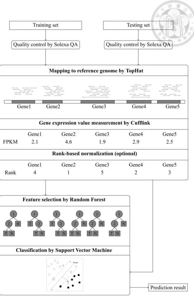
Though RNA-seq technology is popular recently, still few institutions can conduct enough experiments for effective analysis because of the high cost of experiment or lack of samples. Hence, the cross-laboratory or cross-platform analysis become more and more important. The datasets we used are downloaded from Gene Expression Omnibus or Eu- ropean Nucleotide Archive. Owing to the datasets coming from different laboratories or NGS platforms, we will apply sample-wise rank-based normalization to avoid biases from different experimental conditions after measuring the gene expression value. For each dataset, we conduct the quality control of raw reads, filtering low quality reads and too short reads. Next, we map the reads to reference genome (hg19) by TopHat [42] and use Cufflinks [41] to measuring the gene expression value with gene annotation provided by UCSC genome browser. TopHat and Cufflinks have been widely used in a number of recent RNA-seq DGE analysis [41, 34, 43]. After calculate RPKM or FPKM value, we take the next step of cross-laboratory normalization. We use rank-based normalization to transfer expression level to rank level, but this step is optional.

For the following procedures, we will define the training set and testing set first. There are three ways to define the training/testing datasets. First, two datasets are chosen: one as training and the other as testing. Second, three datasets are combined as training and the remaining one as testing. Third, three datasets are chosen for leave-one-out cross- validation (LOO CV): one sample of three datasets is chosen for testing data, and the other for training data. All the samples of the dataset will be chosen for one time. Every

(18)

..

Training set

.

Testing set

.

Quality control by Solexa QA

.

Quality control by Solexa QA

.

Gene1 .

Gene2 .

Gene3 .

Gene4 .

Gene5 .

Mapping to reference genome by TopHat

. Gene expression value measurement by Cufflink .

Gene1 .

2.1 .

Gene2 .

4.6 .

Gene3 .

1.9 .

Gene4 .

2.9 .

Gene5 .

2.5 .

FPKM .

Rank-based normalization (optional) .

Gene1 .

4 .

Gene2 .

1 .

Gene3 .

5 .

Gene4 .

2 .

Gene5 .

3 .

Rank .

Prediction result .

Feature selection by Random Forest .

. . 1.

....

. . N .

..

. . 2.

....

. . . N

..

. . T

.

. . 1.

....

. . 2.

....

. . . N

..

. . T .

..

. . T

.

. . 1.

....

. . 2.

....

. . . N

..

. . T .

..

. . T

.

. . 1.

....

. . N .

..

. . 2.

....

. . . N

..

. . T

.

. . 1.

....

. . N .

..

. . 2.

....

. . . N

..

. . T

.

. . 1.

....

. . N .

..

. . 2.

....

. . . N

..

. . T

.

Classification by Support Vector Machine .

Figure 2.1: Flowchart of the feature selection on cross-laboratory RNA-seq data.

(19)

pair of training set and testing set undergoes below experimental procedure.

From the training datasets, we obtain a significant gene list through the feature selection method, Random Forest. We change the number of selected significant genes from 5 to 250 by an interval of 5. Then, we utilize support vector machine for the classification analysis. The balanced accuracy is used to evaluate the results. The whole workflow is described in Figure 2.1, and details of our methods is described in the following subsec- tions.

2.1 NGS data collection

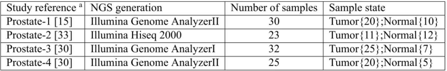
Four datasets are from different laboratories or NGS platform. The first dataset, Prostate- 1, is from [15] which adopts Illumina Genome AnalyzerII. There are 30 samples in Prostate- 1, including 20 for tumor samples and ten for normal samples. The seconed dataset, de- noted as Prostate-2, is from [33]. Prostate-2 contains 11 tumor samples and 12 normal samples obtained from Shanghai Changhai Hospital. It has 28 samples originally, but five of 28 samples do not be provided for download. Prostate-2 uses Illumina Hiseq 2000. The last two Prostate-3 and Prostate-4 are from [30]. Prosate-3 and Prostate-4 come from one institute, and there are 42 tumor samples and 15 normal samples. However, 32 samples are obtained from Illumina Genome AnalyzerI, and the left 25 samples are from Illu- mina Genome AnalyzerII. Hence, we separate 57 samples into two datasets. 32 samples generated by Illumina Genome AnalyzerI are assigned to Prostate-3, and the others are Prostate-4. The details of the above four datasets are summarized in Table 2.1

Table 2.1: Key characteristics of the analyzed data.

Study reference^a NGS generation Number of samples Sample state

Prostate-1 [15] Illumina Genome AnalyzerII 30 Tumor{20};Normal{10}

Prostate-2 [33] Illumina Hiseq 2000 23 Tumor{11};Normal{12}

Prostate-3 [30] Illumina Genome AnalyzerI 32 Tumor{25};Normal{7}

Prostate-4 [30] Illumina Genome AnalyzerII 25 Tumor{20};Normal{5}

a URLs for datasets download:

Prostate-1:http://www.ebi.ac.uk/ena/data/view/SRP002628 Prostate-2:http://www.ebi.ac.uk/ena/data/view/ERP000550

Prostate-3:http://www.ncbi.nlm.nih.gov/geo/query/acc.cgi?acc=GSE25183 Prostate-4:http://www.ncbi.nlm.nih.gov/geo/query/acc.cgi?acc=GSE25183

(20)

2.2 Data pre-processing

Next generation sequencing technology also known as high-throughput sequencing means to generate large amount of sequence data in one run. However, with generating a lot of sequence data, the number of incorrect base calling is also soaring. Therefore, quality control of sequence data generated from NGS technology is extremely important for sequence analysis. Further, highly efficient and fast processing tools are required to handle the large volume of datasets. Here, we use Phred quality score to assess the read quality and SolexaQA toolkit be choosed for the step of quality chontrol.

2.2.1 Phred quality score

In the next-generation sequencing analysis, the quality of each base of sequence is important to each process of whole experiment. Sequencing quality metrics can provide important information for sequencing analysis and it is critical to many downstream pro- cesses, such as base calling, library preparation, read alignment, and variant detection [10].

For measuring sequence quality, Phred quality score is the most common metrics in assess- ing the accuracy of a sequencing platform. Phred quality score is originally designed by the program Phred for aiding the DNA sequencing in the Human Genome Project. Phred quality score has become widely accepted to characterize the quality of DNA sequences, and can be used to compare the efficacy of different sequencing methods. It indicates the probabillity that a given base is called correct by the sequencing machine.

Phred quality scores Q are defined as a property which is logarithmically related to the base-calling error probabilitie P . Quality score Q is calculated by Eq. 2.1.

Q =−10 log₁₀P (2.1)

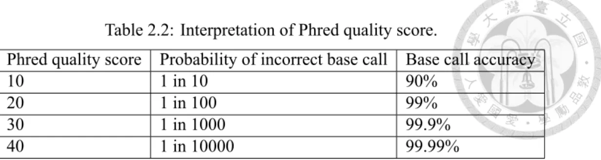
Quality scores range from 4 to about 60, with higher values corresponding to higher quality, as shown in the Table 2.2. For example, if quality score Q is assigned to 30 for a base, it guarantees that the probabillity of an incorrect base call is one in 1000 times. This means that the base call accuracy or the probabillity of a correct base call is 99.9%. While

(21)

Table 2.2: Interpretation of Phred quality score.

Phred quality score Probability of incorrect base call Base call accuracy

10 1 in 10 90%

20 1 in 100 99%

30 1 in 1000 99.9%

40 1 in 10000 99.99%

the quality score is set to 20, it means that the probabillity of incorrect base call is 99%, and it will likely contains an error base for every 100 bp (base pair) sequencing read. High quality score can provide more confidence to whole experiment. On the other hand, low quality score may result in inaccurate conclusion and high cost for validation experiments.

2.2.2 Quality control

For the step of quality control, we use SolexaQA toolkit (http://solexaqa.sourceforge.

net). First, low quality reads (Phred score < 20) are trimmed by DynamicTrim which is provided by SolexaQA toolkit. In this process, each read is croped to its longest contiguous segment if the quality scores are greater than a threshold. We set the threshold to 20 in this work. For example, there is a read quality string as follow (30,30,30,30,10,30,25,30,30,30,10).

The fifth base and 11th base will be croped due to the quality scores of these two bases are smaller than the threshold. Then the string is divided into two substrings (30,30,30,30), (30,25,30,30,30). The second substring is longer than the first one, so the original string is trimmed to the substring (30,25,30,30,30). After trimming process, some reads will be trimmed too short. Thses reads might not only increase the running time of but also the error rate . Therefore, we only preserve the reads which their lengths are longer than 20 bp on both ends of pair-end format for further analysis.

2.3 Mapping to reference genome

Due to the process of RNA splicing, introns in pre-mRNA are removed, and only exons and UTRs are transformed to the final mature mRNA. The RNA spicing not only removes some introns, but also composes some exons to the mRNA or the transcript. Therefore,

(22)

exon 1 ... _{exon 2} _{exon 3} _{exon 4} _{exon 5} _{exon 6} _{exon 7} _{exon 8}

Mapping pair-ended reads to transcriptome

.

exon 1

.

exon 2

.

exon 3

.

exon 5

.

exon 6

.

exon 8

.

transcript

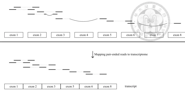
Figure 2.2: RNA-seq reads are mapped to reference genome for detecting the splicing form. In the upper half figure, blocks are exons, gaps between exons are introns, and the thick black line beneath exons represent reference genome. To detect transcript splicing form, we map the reads to each exon. Exons which have no mapping reads are omitted one gene may has some different transcripts because of RNA-spicing. Then, mapping RNA-seq sequences to reference genome must detect the spicing cite. Figure 2.2 is the detail of mapping reads to reference genome. The blank between exons is intron. Here we want to map pair-end reads to reference genome, and find the structure of the transcript.

The aligner will detect the splicing cite, and map reads to reference sequence. The exon which is not mapped will be removed, and the left exons will be gathered into a transcript.

The detection of spicing cite is difficult, so some aligners are designed to RNA-seq reads specifically.

There are several aligners to map RNA-seq reads to reference genome, like GSNAP (Genomic Short-read Nucleotide Alignment Program) [50], Stampy [22] and TopHat [42].

These are the mostly used three aligners in RNA-seq analysis. Some studies have discussed the difference and performance among these three methods [28].

TopHat, which is one of the most commonly used for RNA-seq analysis, is chosen for the aligner in our study. TopHat uses Bowtie [17] to map short reads to reference genome and TopHat have the procedure to detect potential transcript splicing form. The reference genome we used is hg19 download from the UCSC website.

(23)

2.4 Quantifying gene expression value

.

Gene A... Gene B

mapped reads : 20 .

length : 8 kb .

mapped reads : 10 .

length : 4 kb .

Gene A:

Total gene reads = 20 million Total mappped reads = 30 million Gene length = 8 kilobases

RPKM = 20/(30*8) = 0.083 .

Gene B:

RPKM = 10/(30*4) = 0.083

(a) Sample A

.

Gene A... Gene B

mapped reads : 10 .

length : 8 kb .

mapped reads : 5 .

length : 4 kb .

Gene A:

RPKM = 10/(15*8) = 0.083 .

Gene B:

RPKM = 5/(15*4) = 0.083

(b) Sample B

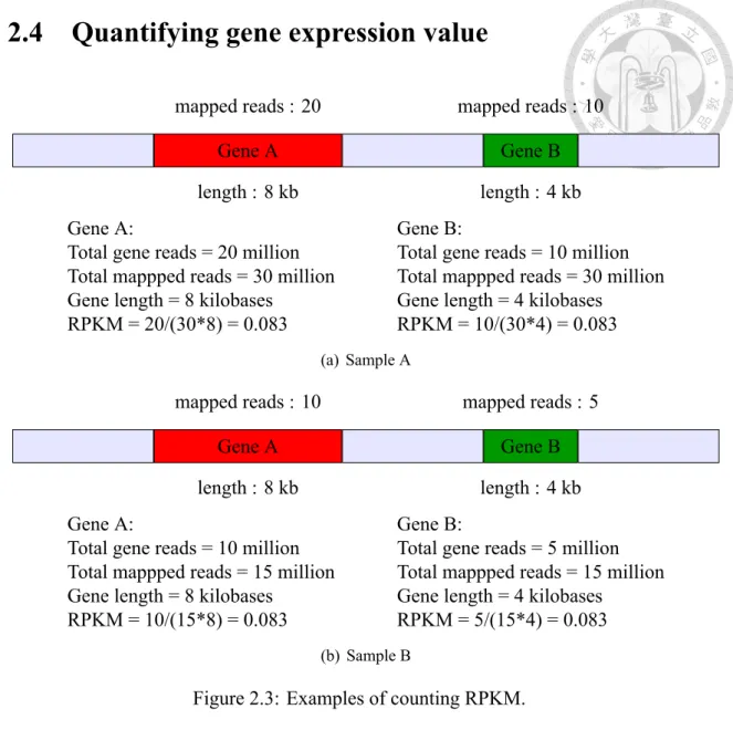
Figure 2.3: Examples of counting RPKM.

RNA-seq technology uses read count of gene to quantify the gene expression value.

Basically, read count reflects the expressed level of a gene. Only concern the read count may have some biases because the length of genes are different. The longer gene may be mapped by more reads than the gene which is shorter. The second reason is that the total reads between samples are not the same. More total reads of the sample may result in more reads be mapped to the gene. We use Read Per Kilobase of transcript per million mapped reads (RPKM) for single-end data and Fragment Per Kilobase of transcript per Million mapped reads (FPKM) for pair-end data to solve above bias. RPKM (FPKM) is calculated by Eq. 2.2.

RPKM = total gene reads

total mapped reads(million)× gene length (2.2)

(24)

Total gene reads are the reads mapped to the gene. Total mapped reads are all reads that be mapped to the transcriptome, and the unit is million. Gene length is how many bases the gene contains. Total gene reads divided by total mapped reads means that how many partitions of reads are mapped to the gene. Next, it has to be divided by the gene length, because the gene with longer length will be mapped by more reads. For example, there are two genes in sample A in Figure 2.3(a). The length of Gene A is 8 kilobases, and Gene B is 4 kilobases. There are 20 million reads and 10 million reads which are mapped to Gene A and Gene B, respectively. For Gene A, total gene reads is 20 million; mapped reads is 30 million; gene length is 8 kilobases. The value of RPKM of Gene A equals to 20/(30∗ 8) = 0.083. Total gene reads of Gene B is 10 million, and the length of Gene B is 4 kilobases. The value of RPKM of GeneB equals to 10/(30∗ 4) = 0.083, too. Total reads of Gene A is more than the total reads of Gene B, but the length of Gene B is shorter than Gene A. Therefore, the expressed level of a base of Gene A is equal to Gene B. Next, we compare sample A with sample B in Figure 2.3(b). Both gene length of sample B are equal to sample A, but the reads mapped to Gene A and Gene B are half of sample A. The RPKM value of Gene A of sample B is 0.083 which is euqal to the RPKM of Gene A of sample A. The reads mapped to Gene A of sample A is more than the one of sample B, but the expressed level is equivelant. Because the total mapped reads to transcriptome of sample A is two times to smaple B, the reads mapped to a gene may increase two times, too. Using RPKM to quantify gene expressed level can avoid the bias which is resulted from difference of gene length and sequencing depth.

RPKM and FPKM are almost the same thing. RPKM stands for Reads Per Kilobase of transcript per Million mapped reads, and FPKM stands for Fragments Per Kilobase of transcript per Million mapped reads. The difference between RPKM and FPKM is that RPKM calculates how many reads be mapped on a gene, but FPKM calculates how many fragments rather than read count. Paired-end RNA-Seq experiments produce two reads per fragment. Normally, fragment will be mapped two times, then it will double count the fragment. However, if one of the pair reads has poor quality, then we may count this fragment only one time, but some fragments two. Therefore, using FPKM is more

(25)

appropriate for analysing pair-end data.

In our study, we use Cufflinks (http://cufflinks.cbcb.umd.edu/index.html) to calculate RPKM and FPKM. Cufflinks uses reads which is mapped to reference genome by TopHat to calculate RPKM or FPKM for each gene.

2.5 Cross-laboratory normalization

The goal of cross-laboratory in DGE analysis is that whether models bulit from dataset of one laboratory can differentiate dataset of another. Moreover, we can combine all the datasets from different laboratories to a huge dataset, and use it to differentiate another dataset. However, in high throughput technology, there are lots of difference among the datasets published by different laboratories, such as enviroments, machines, sample races, and many experiment conditions [23, 12]. The datasets from different laboratories may have different distribution in raw data. If we comprise these datasets directly, it will influence the result strongly. It has to be normalized between datasets to the same distribution before further analysis [19].

Not only cross-laboratory may have huge influence, but also cross-platform. Several studies show that even using the same samples, the measurements from different platforms are still poorly correlated [2, 18]. Therefore, many researches have been conducted to reduce the bias which is resulted from cross-laboratory or cross-platform. Many approaches have been proposed to solve this bias in microarray technology, such as log transform [5], mean scale, rank-based normalization [52]. In RNA-seq technology, still few research discuss the normalization problem across laboratories or platforms [16, 35]

Many studies have shown that the rank-based normalization is effective to raise prediction accuracy and let it more stable than only using expression values. Expression values may be biased because the scale of each gene may vary among different experimental en- vironments. To rank gene’s order of a sample instead of using its expression value is much better to eliminate systematic biases and improve the prediction accuracyn [52]. There are several variants of rank-based normalization. First, the basic type of rank-based normalization which we used in our study, only use the rank of gene in one sample to replace the

(26)

expression value of the gene [44]. Second, median rank is another rank-based normalization. It calculates the median of each gene between the samples and sorts those medians as the value of rank [47]. Another rank-based normalization is quantile normalization [3].

The value of rank is measured by taking the average of the expression values of defined rank in samples, and then replaces the expression value of each gene by the value of its rank. Some researches show that using simple rank-based normalization performs better than quantile normalization method [44, 31]. Then, we choose the simple rank-based normalization. Using the gene’s rank in the sample to replace the expression value. In this study, we use both RPKM (FPKM) and rank levels for feature selection to observe the improvement by applying rank-based normalization. After this procedure, we use RPKM and rank value to do the step of feature selection.

(27)

Chapter 3 Feature selection and classification

Finding relevent genes from tens of thousands of genes is an important and difficult task in differetial gene analysis. We apply an embedded feature selection method, Random Forest [4] to select a relevent gene list from the training set. Then, we evaluat the gene list by checking classification accuracy of testing set by the well-known classifier, Support Vector Machine (SVM) [7]. We will introduce the details of these two techniques in the folowing sections.

3.1 Feature selection by Random Forest

Random Forest which is first proposed by Breiman [4] is an embedded feature selection method which interacts with classifier. We apply Random Forest for feature selection on training set to obtain a ranking list of gene which is sorted from the most relevent to the least relevent for classification. We use the ‘randomForest’ [20] of R-package for this step. In this section, we first introduce the decision tree which Random Forest uses, and ensemble of all dicision trees. Finally, we introduce the whole procedure of Random Forest.

3.1.1 Building decision tree

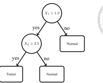
Decision tree is a predictive model which can be used in classification or regression.

Here we use the classification tree. Figure 3.1 is the structure of a classification tree.

(28)

X1> 1.3...

Normal

.

X2> 2.5

.

Normal

.

Tumor

.

no .

yes .

no .

yes

Figure 3.1: An example of a decision tree.

Assume that a data A has a feature vector X = (x₁, x₂, ..., x_p) which is a p-dimensional vector. We want to predict the class Y = {1, −1} of A from the feature vector X. The classification tree is a binary tree, and each internal node represents a test to A. At each internal node of the binary tree, we apply the test to get the outcome (yes or no) to decide which way A has to go. If the test return yes, then A goes to the left branch, and A goes to the right branch otherwise. Finally, A reaches the leaf node, where we make a prediction of class Y.

Constructing classification or regression tree is based on greedy algorithms. The classification tree is constructed top-down, starting from a root node. For choosing the internal node, we calculate the value of:

|S| · H(S) − |St| · H(St)− |Sf| · H(Sf), (3.1)

where S denotes the set of samples that reach the node, S_tand S_f denote the subset of S which the the test is true and false, respectively. The function H is the Shannon entropy:

H(S) = −

∑Y i=1

p(c_i)· log2p(c_i), (3.2)

where Y is the number of class and p(ci) is the proportion of samples in S belonging to class c_i. The feature which maximizes the Eq 3.1 will be chosen for the internal node, and remove from the feature vector. The tree is constructed recursively, until all the features

(29)

are assigned for internal node.

3.1.2 Ensemble of trees

Ensemble method is to aggregate the prediction of several trees, and usually improves the performance of a single tree. The goal of ensemble method is to use diversified models

to reduce the variance. Random Forest is an ensemble of N decision trees{T1(X), T₂(X), ..., T_N(X)}, where X = (x₁, x₂, ..., x_p) is a p-dimensional vector of features. The ensemble outputs

{ ˆY1 = T₁(X), ..., ˆY_N = T_N(X)}, where ˆYi(i = 1, ..., N ) is the prediction result of the tree T_i. The outputs of all trees are aggregated to produce one final prediction which is a vajority vote of trees for classification problem.

3.1.3 Training procedure

Given data on a set of size n, D ={(X1, Y₁), (X₂, Y₂), ..., (X_n, Y_n)}, where Xiis the feature vector and Y_i is the class label of sample i. The training procedure of Random Forest is as follow:

1. From training data of n sample, random sampling N subsets with replacement from n samples.

2. For each subset, build a decision tree with the following rule: at each internal node choose the gene which can split the subset best.

3. Repeat above steps until all N trees are constructed well. In our study, we set N to 1000.

3.1.4 Measuring feature importance

Breiman has proposed a procedure to compute the feature importance. Consider out- of-bag samples S_owhich are the training samples that are not in the samples which be used in the construction of emsemble trees. The prediction accuracy p_iof S_o, where i stands for the i-th tree. Randomly permute the value of gene j in S_oto get S_o_j After permutation, we

(30)

get the predition accuracy p_i_j of S_o_j. We can get the importance s_j of gene j to average all the value of p_i substrct p_i_j. At last, sort the important list, and get the top 250 genes for calssification.

3.2 Classification

To evaluate the performance of feature selection method, the best way is to perform the classification with the optimal feature set which is selected by feature selection method.

In previous step, We obtained a relevent gene list by applying Random Forest in training set. We use the gene list to classify testing set by the well-known classifier Support Vector Machine [7]. Then, we evalute the perfomance of the gene list by checking the prediction accuracy of the testing set. The package of Support Vector Machine we used is provided by a R-package ‘e1071’ [6].

3.2.1 Introduction of Support Vector Machine

Support Vector Machine, a supervised machine learning technique, has been widely used in various areas of biological classification tasks [7]. SVM is designed for binary classification originally, but several methods have been proposed to extend binary classification to multi-class calssfication. In our stduy, we only consider the binary classification.

The concept of binary SVM is trying to find a hyperplane which can separate all the points apart well. All the points of class A are on one side of the hyperplane, and the points of class B are on another side. There are many hyperplane to separate n points to two classes. The best separating hyperplane H is with the largest separation, or margin, between the two classes. The margin means the distance of H to the nearest point on each side.

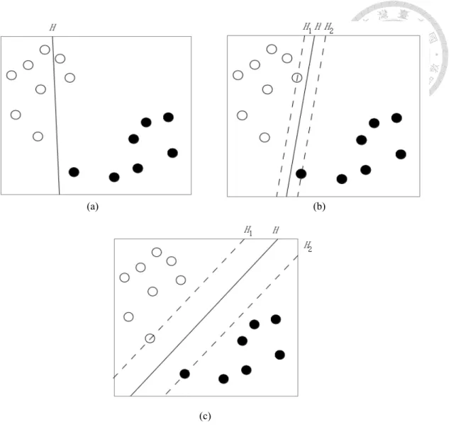
For example, there are 15 points on a plane in Figure 3.2. Eight of them are white, and the other seven are black. In Figure 3.2, there are three hyperplanes to separate these 15 points. H is the hyperplane, and the distance between H₁and H₂ is the margin. In Figure

(31)

(a) (b)

(c)

Figure 3.2: Classification of 15 points.

3.2(a), the hyperplane H is not a good way to separate points, because two white points are separated to the wrong side. The hyperplane H of Figure 3.2(b) and Figure 3.2(c) can separate points to two sides well, but the H in Figure 3.2(c) is better than Figure 3.2(b), because the margin in Figure 3.2(c) is larger.

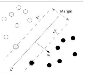
Then, consider n training points: S ={(xi, y_i)}, i = 1, ..., n, where xi ∈ R^pis a vector of feature of i-th sample, and y_i is the class label of sample x_i. For binary classification problem, y_i ∈ {−1, 1}. The goal is to find the maximum-margin hyperplane that divides the points into two parts which are y_i = 1 and y_i = −1. In Figure 3.3, assume the hyperplane H is w^Tx− b = 0, and H1 and H2 are w^Tx− b = 1 and w^Tx− b = −1, respectively. The vector w is the normal vector to the hyperplane H. Then, the margin is

(32)

Figure 3.3: Illustration of SVM classification.

the distance between H₁and H₂, _||w||² . All n points will satisfied the following constraints:

w^Tx_i− b ≥ 1 for all yi = 1 w^Tx_i− b ≤ −1 for all yi =−1.

We can combine above two constraints to:

y_i(w^Tx_i− b) ≥ 1 for all 1 ≤ i ≤ n.

Maximizing the _||w||² equals to minimizing ¹₂||w||. Then, finding the largest margin prob- lem becomes to the following optimization problem:

minimize 1 2w^Tw

subject to y_i(w^Tx_i− b) ≥ 1 for i = 1, 2, ..., n (3.3)

Using Lagrange Multiplier Method, this optimization problem can be solved by solving the dual problem, a quadratic problem to get the hyperplane. After obtaining the optimal hyperplane to separate training data, we can use this model to predict the testing data.

(33)

3.2.2 Classification using SVM

We evaluate the feature selection method and rank-based normalization by SVM classification accuracy. Here, we use the ‘e1071’ of R package for SVM. There are three types of training set and testing set which we mentioned before.

All pairs of training and testing datasets undergo this procedure. After feature selection for training set, we use SVM to get the training model from training set and use this model to predict the testing set.

3.3 Evaluation

For classification, the most commonly used prediction mesurement is accuracy. How- ever, for unbalaced data, a high accuracy by predicting all data to the major class may be misleading. For example, Prostate-3 has 25 tumor samples, but only 7 normal samples.

Prostate-4 is also unbalaced dataset, 20 for tumor samples, and five for normal samples.

Therefore, we use balanced accuracy for our measurements:

Balanced accuracy = 1 2·

( TP

TP + FN + TN TN + FP

)

where TP, TN, FP and FN indicate numbers of true positive, true negative, false positive and false negative. True positive means the sample which is positive and be predicted as positive. True negative means the sample which is negative and be predicted as negative.

False positive means the sample which is negative and be predicted as positive. False negative means the sample which is positive and be predicted as negative. _{T P +F N}^{T P} is true positive rate which measures the proportion of actual positives which are correctly predicted, and_{T N +F P}^{T N} is true negative rate which measures the proportion of actual negatives which are correctly predicted. If the classifier predict all data to major class, the balaced accuracy will be only 50%. Hence, balanced accuracy can avoid inflated performance estimates on imbalanced dataset. Therefore, it is generally believed that the balanced accuracy better handle the data imbalance and can reveal the performance on cancer classification.

(34)

Chapter 4 Results

In this chapter, we will show all experimental results in figures and tables. The first result is the comparison of classification performance of three methods:

1. using FPKM for gene expression value and Random Forest for feature selection 2. applying rank-based normalization and Random Forest for feature selection 3. using Cuffdiff for feature selection

It is observed that the results of applying rank-based normalization outperform the other two in most figures and tables. Moreover, we discuss the influence of cross-laboratoy on feature selection. The performance is stable and very high with few selected gene in LOO CV test, but to reach the high performance the number of selected gene must be more than 125 in cross-laboratory prediction. Furthermore, the prediction may be influenced by the sequencing platform. It leads the poor performance when Prostate-3 is the training dataset, and the high performance when Prostate-2 is used for training.

4.1 Results of performance

In Section 2.5, we introduced the rank-based normalization. Some studies of microarray analysis indicated that the classification accuracy with rank-based normalization is better than using expression values. In our study, we futher demonstrate that rank-based normalization is also better than using FPKM in cross-laboratory prediction.

(35)

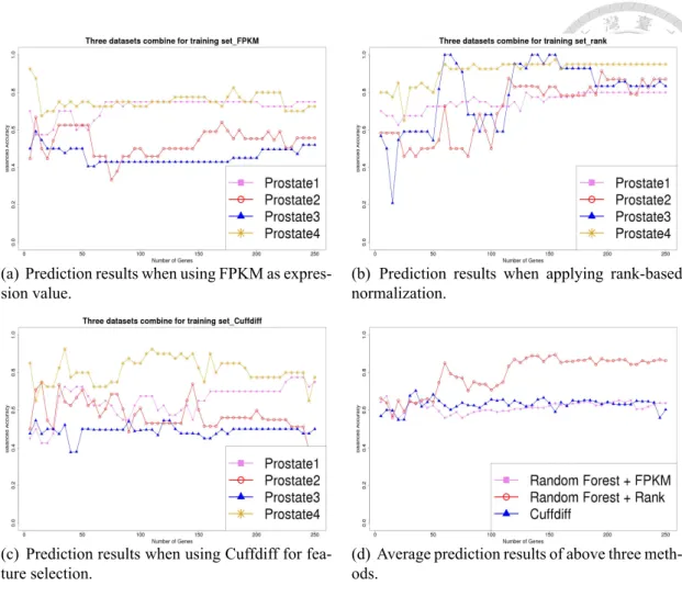
(a) Prediction results when using FPKM as expression value.

(b) Prediction results when applying rank-based normalization.

(c) Prediction results when using Cuffdiff for feature selection.

(d) Average prediction results of above three methods.

Figure 4.1: Results of prediction balanced accuracy. Three data sets are combined as the training data set. The remaining one shown in the legend is regarded as the testing data set.

In Figure 4.1, each line stands for the balanced accuracy curve of combining three datasets for training set and one for testing set. For example, the pink line in Figure 4.1(a) is the balanced accuracy curve of using Prostate-2, Prostate-3 and Prostate-4 for training set and predicting Prostate-1. Figure 4.1(a) is the result of using FPKM for gene expression value and Figure 4.1(b) is the result when applying rank-based normalization.

Figure 4.1(a) shows that the balanced accuracy of using FPKM is on the range of 50%

to 70%. However, the curve when using rank-based normalization is raised evidently at gene number more than 125. In Figure 4.1(b), the balanced accuracy reached to 90% to 100% at number of gene more than 125 in testing Prostate-3 and Prostate-4, and predicting Prostate-1 and Prostate-2 also raised to 80% to 85%. All four combination of training and testing sets have evident raise from using FPKM or RPKM to rank-based normalization.

Figure 4.1(d) is the average balanced accuracy of four combination in Figure 4.1(a)-(c).

(36)

For example, the red line of Figure 4.1(d) is the average prediction result of applying rank- based normalization and using Random Forest for feature selection. From Figure 4.1(d), we can observe the clear increase of balanced accuracy after gene number is more than 125. Table 4.1 concluded the highest balanced accuracy and highest average balanced accuracy. The highest average balanced accuracy means the highest point in Figure 4.1(d).

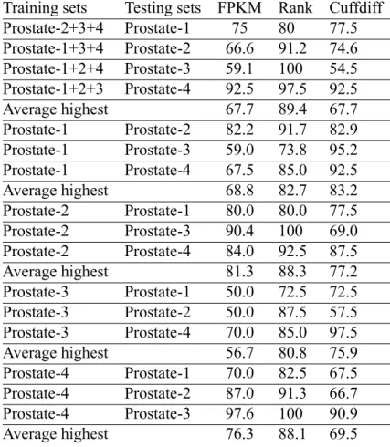
Predicting Prostate-2 and Prostate-3 have the most growth, almost increasing 40%. For the average of four combination of combine three datasets for training set, the highest balanced accuracy of FPKM is only 67.7%, but rank-based normalization is 89.4%.

Figure 4.2 is the result of using one dataset for training set to predict another testing dataset. The left figures of Figure 4.2 are the result of using FPKM, and the right figures are using rank-based normalization. In Figure 4.2(a), balanced accuracy of predicting Prostate-3 and Prostate-4 increase to 75% and 80%, and predicting Prostate-2 reaches to 90%. The balanced accuracy of predicting Prostate-3 have a large increase from 50% to 100% in Figure 4.2(b). In Figure 4.2(d), all the curve have a great improvement after applying rank-based normalization. Although the highest balanced accuracy of training Prostate-2 to predict Prostate-1 and Prostate-4 have no improvement, it becomes more stable after applying rank-based normalization.

In Figure 4.1 and Table 4.1, we can observe that almost all the performance improves with rank-based normalization, but the performance is still poor when training data is Prostate-3. The reason for the poor performance of training Prostate-3 to predict others might be that the distribution of Prostate-3 is far from others or the special property of Prostate-3. We will discuss this situation in Section 4.3.

Next, we compare the performance of using well-known differetial gene analysis tool, Cuffdiff, with the performance of Random Forest after applying rank-based normalization.

We sort the p-value which calculated by Cuffdiff in ascending order, and choose the top 250 genes for classification. The results of using Cuffdiff for feature selection are in Figure 4.1(c) and Figure 4.3, and it is similar to the result of using Random Forest without rank-based normalization. It performs better in predicting Prostate-4 than Random Forest without rank-based normalization, but the performance of predicting Prostate-1 is worse.

(37)

Figure 4.1(d) shows the performance of using Cuffdiff and using Random Forest without rank-based normalization are both around 60%. The performance of applying rank-based normalization is higher than others at gene number more than 50. Therefore, the rank- based normalization is effective in cross-laboratory feature selection.

Table 4.1: Results of highest balanced accuracy.

Training sets Testing sets FPKM Rank Cuffdiff Prostate-2+3+4 Prostate-1 75 80 77.5 Prostate-1+3+4 Prostate-2 66.6 91.2 74.6 Prostate-1+2+4 Prostate-3 59.1 100 54.5 Prostate-1+2+3 Prostate-4 92.5 97.5 92.5

Average highest 67.7 89.4 67.7

Prostate-1 Prostate-2 82.2 91.7 82.9 Prostate-1 Prostate-3 59.0 73.8 95.2 Prostate-1 Prostate-4 67.5 85.0 92.5

Prostate-2 Prostate-1 80.0 80.0 77.5 Prostate-2 Prostate-3 90.4 100 69.0 Prostate-2 Prostate-4 84.0 92.5 87.5

Prostate-3 Prostate-1 50.0 72.5 72.5 Prostate-3 Prostate-2 50.0 87.5 57.5 Prostate-3 Prostate-4 70.0 85.0 97.5

Prostate-4 Prostate-1 70.0 82.5 67.5 Prostate-4 Prostate-2 87.0 91.3 66.7 Prostate-4 Prostate-3 97.6 100 90.9

4.2 Influence of cross-laboratory

Figure 4.4 is the LOO CV results of combining three datasets with applying rank- based normalization. The leave-one-out cross-validation (LOO CV) means that it uses one sample for testing set and the others for training set, and each sample has the turn for testing. Then, the validation results are averaged over all rounds. For example, the pink line in Figure 4.4 is the result of using Prostae-2, Prosate-3 and Prostate-4 for LOO CV. 79 of the total 80 samples use for training set, and the left one is for testing. In LOO CV test, the balanced accuracy is stable at low selected gene number, but it needs to be more than

(38)

(a) The training data set is Prostate-1.

(b) The training data set is Prostate-2.

(c) The training data set is Prostate-3.

(d) The training data set is Prostate-4.

Figure 4.2: Results of prediction balanced accuracy. The training data set is shown on each subfigure title, and the testing data set is described in legend.

(39)

(a) The training data set is Prostate-1. (b) The training data set is Prostate-2.

(c) The training data set is Prostate-3. (d) The training data set is Prostate-4.

Figure 4.3: Results of prediction balanced accuracy when using Cuffdiff for feature selection. The training data set is shown on each subfigure title. And the testing data set is described in legend.

125 in cross-laboratory feature selection. Due to distribution of four sets is independent, then prediction across sets is difficult. In addition to the laboratories and platforms are different, the races of samples are different between datasets. Research shows that even the same dataset and the same laboratory will get different results by different platforms. In LOO CV test, the training model learns from different laboratoies which the testing sample belongs to. Then, it is easy to choose the features to classify testing sample. Therefore, it can get the high performance when the selected genes are few.

4.3 Influence of NGS platforms

Although rank-based normalization can rescale cross-laboratory data, the performance is still poor in Figure 4.2(c). The reason may be the sequencing machine which generating Prostate-3 is older than others. Prosate-3 is generated from Illumina Genome Analyzer I

(40)

Figure 4.4: Results of LOOCV when using rank-based normalization.

(GAI), but Prostate-1 and Prostate-4 are both using Illumina Genome Analyzer II (GAII) and Prostate-2 is using Illumina Hiseq 2000 which is the newest machine. The detail of four datasets and platforms are summarized in Table 4.2. Prostate-3 is single-end data which has higher error rate than pair-end data during mapping to reference genome, and the read count per sample is also fewer than others. The read count of a sample in Prostate- 3 is only 5.3M which is far less than the others. Although the scheme of RPKM (FPKM) adjust the bias result from different total read count, the few read count may result in many genes ummapped by reads. On the other hand, Prostate-2 performs well in low number of selected genes, and the performance is stable. The read count and base count of each sample in Prostate-2 are far more than other datasets, and Illumina Hiseq 2000 which generates Prostate-2 provides lower error rate and higher perfomance than other platforms. By the advatage of platform, the information provided by Prostate-2 is more stable and it can provide feature selection higher performance. Therefore, not only the cross-laboratoty will affect performance of feature selection, but also the platform used is the factor.

(41)

Table4.2:Detailsofdatasetsandplatforms. StudyreferenceNGSgenerationreadtypeAverageAveragereadlength readcountbasecount Prostate-1[15]IlluminaGenomeAnalyzerIIpairend11M0.8G36bp Prostate-2[33]IlluminaHiseq2000pairend34M6.3G100bp Prostate-3[30]IlluminaGenomeAnalyzerIsingleend5.3M0.2M36bp Prostate-4[30]IlluminaGenomeAnalyzerIIpairend12.5M1G36bp

(42)

Chapter 5 Conclusions and future work

In our study, we apply rank-based normalization to reduce the influence by cross- laboratory. The performance has a great improvement after appying rank-based normalization. Furthermore, the performance of using Random Forest with applying rank-based normalization is better than using the well-known differential gene tool Cuffdiff. Although the prediction result has been improved by rank-based normalization, the balanced accuracy is still not good enough. To further improve the performance, it may use better machine which generates the sequence data. We have discussed that the sequencing machine is also an important factor which affects the preformance of feature selection on cross-lab RNA-seq datasets. The better platform provide more effective and stable information for feature selection, and it performs well in the prediction results. Hence, by the development of RNA-seq technology, the data generated by the newer machine would be more suitable for cross-laboratory analysis.

RNA-sequencing technology provides expression level of genes and sequence structure of RNA. In our study, we only use gene expression and we want to take an advantage of sequence structure to further analysis. Next, we want to apply the cross-laboratory feature selection in gene fusion detection. The gene fusion occurs frequently in prostate cancer Gene fusion means that two previously separated genes fuse together to a new gene. Due to the dataset are across different laboratories and different races, we are able to detect the common gene fusion event in specific race or among different races.

(43)

Bibliography

[1] S. Anders and W. Huber. Differential expression analysis for sequence count data.

Nature Precedings, (713), 2010.

[2] T. Bammler, R. P. Beyer, S. Bhattacharya, G. A. Boorman, A. Boyles, B. U. Bradford, R. E. Bumgarner, P. R. Bushel, K. Chaturvedi, D. Choi, M. L. Cunningham, S. Deng, H. K. Dressman, R. D. Fannin, F. M. Farin, J. H. Freedman, R. C. Fry, A. Harper, M. C. Humble, P. Hurban, T. J. Kavanagh, W. K. Kaufmann, K. F. Kerr, L. Jing, J. A. Lapidus, M. R. Lasarev, J. Li, Y.-J. Li, E. K. Lobenhofer, X. Lu, R. L. Malek, S. Milton, S. R. Nagalla, J. P. O’Malley, V. S. Palmer, P. Pattee, R. S. Paules, C. M.

Perou, K. Phillips, L.-X. Qin, Y. Qiu, S. D. Quigley, M. Rodland, I. Rusyn, L. D.

Samson, D. A. Schwartz, Y. Shi, J.-L. Shin, S. O. Sieber, S. Slifer, M. C. Speer, P. S. Spencer, D. I. Sproles, J. A. Swenberg, W. A. Suk, R. C. Sullivan, R. Tian, R. W. Tennant, S. A. Todd, C. J. Tucker, B. V. Van Houten, B. K. Weis, S. Xuan, and H. Zarbl. Addendum: Standardizing global gene expression analysis between laboratories and across platforms. Nature Methods, 2(6):477, 2009.

[3] B. M. Bolstad, R. A. Irizarry, M. Astrand, and T. P. Speed. A comparison of normalization methods for high density oligonucleotide array data based on variance and bias. Bioinformatics, 19(2):185–193, 2003.

[4] L. Breiman. Random forests. Machine Learning, 45:5–32, 2001.

[5] N. Cloonan, A. R. R. Forrest, G. Kolle, B. B. A. Gardiner, G. J. Faulkner, M. K.

Brown, D. F. Taylor, A. L. Steptoe, S. Wani, G. Bethel, A. J. Robertson, A. C.

Perkins, S. J. Bruce, C. C. Lee, S. S. Ranade, H. E. Peckham, J. M. Manning, K. J.

(44)

McKernan, and S. M. Grimmond. Stem cell transcriptome profiling via massive- scale mrna sequencing. Nature Methods, 5(7):613–619, 2008.

[6] E. Dimitriadou, K. Hornik, F. Leisch, D. Meyer, and A. Weingessel. e1071: Misc Functions of the Department of Statistics (e1071), TU Wien. R package version 1.5- 25., 2011.

[7] T. S. Furey, N. Duffy, N. Cristianini, D. Bednarski, M. Schummer, and D. Haussler.

Support Vector Machine Classification and Validation of Cancer Tissue Samples Us- ing Microarray Expression Data. Bioinformatics, 16(10):906–914, 2000.

[8] T. R. Golub, D. K. Slonim, P. Tamayo, C. Huard, M. Gaasenbeek, J. P. Mesirov, H. Coller, M. L. Loh, J. R. Downing, M. A. Caligiuri, and et al. Molecular classification of cancer: class discovery and class prediction by gene expression monitoring.

Science, 286:531–537, 1999.

[9] T. Hardcastle and K. Kelly. Bayseq: empirical bayesian methods for identifying differential expression in sequence count data. BMC Bioinformatics, 11, 2010.

[10] I. Inc. Quality Scores for Next-Generation Sequencing - Illumina. 2001.

[11] I. Inza, P. Larrañaga, R. Blanco, and A. J. Cerrolaza. Filter versus wrapper gene se- lection approaches in DNA microarray domains. Artificial intelligence in medicine, 31(2):91–103, 2004.

[12] R. A. Irizarry, D. Warren, F. Spencer, I. F. Kim, S. Biswal, B. C. Frank, E. Gabriel- son, J. G. N. Garcia, J. Geoghegan, G. Germino, C. Griffin, S. C. Hilmer, E. Hoffman, A. E. Jedlicka, E. Kawasaki, F. Martínez-Murillo, L. Morsberger, H. Lee, D. Pe- tersen, J. Quackenbush, A. Scott, M. Wilson, Y. Yang, S. Q. Ye, and W. Yu. Multiple- laboratory comparison of microarray platforms. Nature Methods, 2(5):345–350, 2005.

[13] P. Jafari and F. Azuaje. An assessment of recently published gene expression data analyses: reporting experimental design and statistical factors. BMC Medical Infor- matics and Decision Making, 6:27, 2006.

(45)

[14] A. Jemal, F. Bray, M. M. Center, J. Ferlay, E. Ward, and D. Forman. Global cancer statistics. CA: A Cancer Journal for Clinicians, 61(2):69–90, 2011.

[15] K. Kannan, L. Wang, J. Wang, M. M. Ittmann, W. Li, and L. Yen. Recurrent chimeric rnas enriched in human prostate cancer identified by deep sequencing. Proceedings of the National Academy of Sciences, 108(22):9172–9177, 2011.

[16] J. Kim, K. Patel, H. Jung, W. P. Kuo, and L. Ohno-Machado. Anyexpress: integrated toolkit for analysis of cross-platform gene expression data using a fast interval matching algorithm. BMC Bioinformatics, 12:75, 2011.

[17] B. Langmead, C. Trapnell, M. Pop, and S. L. Salzberg. Ultrafast and memory- efficient alignment of short DNA sequences to the human genome. Genome Biology, 10(3):R25–10, 2009.

[18] J. E. Larkin, B. C. Frank, H. Gavras, R. Sultana, and J. Quackenbush. Independence and reproducibility across microarray platforms. Nat Methods, 2(5):337–344, 2005.

[19] J. T. Leek, R. B. Scharpf, H. C. Bravo, D. Simcha, B. Langmead, W. E. John- son, D. Geman, K. Baggerly, and R. A. Irizarry. Tackling the widespread and critical impact of batch effects in high-throughput data. Nature Reviews Genetics, 11(10):733–739, 2010.

[20] A. Liaw and M. Wiener. Classification and regression by randomforest. R News, 2(3):18–22, 2002.

[21] R. Lister, R. C. O’Malley, J. Tonti-Filippini, B. D. Gregory, C. C. Berry, A. H. Millar, and J. R. Ecker. Highly integrated single-base resolution maps of the epigenome in Arabidopsis. Cell, 133(3):523–536, May 2008.

[22] G. Lunter and M. Goodson. Stampy: A statistical algorithm for sensitive and fast mapping of Illumina sequence reads. Genome Research, 21(6):936–939, 2011.

[23] N. Mah, A. Thelin, T. Lu, S. Nikolaus, T. Kühbacher, Y. Gurbuz, H. Eickhoff, G. Klöppel, H. Lehrach, B. Mellgård, C. Costello, and S. Schreiber. A compar-