LEARNING DECISION FUNCTIONS IN THE FUZZY γ-MODELS
Jung-Hsien Chiang* and Yau-Hwang Kuo
Department of Computer Science and Information Engineering National Cheng Kung University
Tainan, Taiwan
Abstract
In this approach, we investigate the fuzzy γ-models for decision analysis and making. This methodology utilizes fuzzy γ-model as an information aggregation operator.
It provides several advantages due to the fact that the input to each model is the evidence supplied by the degree of satisfaction of sub-criteria and the output is the aggregated evidence. We also generalize fuzzy γ-models as a hierarchical network in this work.
Thus, the decision making process is to aggregate and propagate the evidence information through such a hierarchical network. This trainable network is able to perceive and interpret complex decisions by using those fuzzy models. The simulation study examines the learning behaviors of the fuzzy γ-models using two numerical examples.
key words: Fuzzy Modeling, Aggregation Operator, Neural Networks, Hybrid Systems
_______________________________________________
* corresponding author: [email protected]
1. Introduction
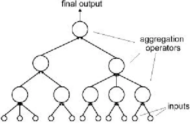
The decision making problem has been receiving a lot of attention in artificial intelligence research recently. From the decision making perspective, the most important and informative aspects of any paradigm are the framework that performs specific computational operations using functionally distinct nodes, which is able to represent knowledge as a hierarchical architecture form. Fig 1 depicts the hierarchical decision network. Most existing neurocomputation systems employ learning algorithms that extract knowledge from examples. However, those paradigms are black-boxes. Both hierarchy information as well as inference characteristics for network interpretation are unavailable. In this paper, we explore the properties of the fuzzy γ-models and their utilization in fuzzy neurocomputation. Adoption of a fuzzy γ-model in network-based representation rather than a traditional neuron leads to an important distinction in how processes of fuzzy models integration are utilized in decision making. This paradigm attempts to use learning algorithm to find appropriate connection parameters in hierarchy.
Fig 1 Example of a hierarchical decision network
Fuzzy models have been applied to neural network implementation in a number of ways. Klir(1995) and Zimmermann(1991) summarized the classes of fuzzy operators based on their aggregation behaviors. Other interesting fuzzy neurocomputation paradigms that have been suggested include the fuzzy-set based neurons (Pedrycz, 1995),
which realize aggregation of the input signals and carry out some referential processing, the ordered weighted averaging (OWA) operator (Yager, 1994; Fodor, 1995), which is capable of performing aggregations according to linguistic quantifiers. More recently, Keller et al. has suggested that additive γ-models with Yager’s operators and with Yager’s operators on exponential inputs can be trained to learn the tasks of function approximation between input and output spaces(Keller, 1994). All of these paradigms have parameters that can be adjusted (or learned) to arrive at desired representation.
Other fuzzy neural networks (Buckly, 1995; Takagi, 1992) are able to perform soft computing in various applications, and the hierarchical aggregation networks (Chiang, 1999; Krishnapuram, 1992), which use the fuzzy connectives in multilayer networks for decision making.
The paper is organized as follows. In Section 2, the basic properties of the fuzzy γ-models are considered. Section 3 presents network implementation and learning of the fuzzy γ-models. The experimental results are presented in Section 4.
2. The Properties of Fuzzy γ-Models
In this section we briefly describe basic fuzzy set operator s and their generalizations. Several properties of the fuzzy γ-models are then discussed.
A. Basic Fuzzy Set Operators
The union of two fuzzy sets is in general a function u: [0, 1] x [0, 1] → [0, 1]
such that it must satisfy the commutativity, monotonicity, associativity, and boundary conditions. Certainly, there are a number of interesting families of union operators in terms of the underlying fuzzy set theory(Kandel, 1986; Kruse, 1994). Two particular interest examples that we consider in this work are:
The maximum operator:
(x x xn) max(x x xn)
u 1, 2,... = 1, 2,...
Yager’s union operator:
( )
= ∑=
n p
j p j
n min x
x x x u
/ 1
1 ,
2 ,
1 ... 1, p∈( )0,∞
An intersection operator i is a function i: [0, 1] x [0, 1] → [0, 1]
such that it also sa tisfy the commutativity, monotonicity, associativity, and boundary conditions. Examples include:
The minimum operator:
(x x xn) min(x x xn)
i 1, 2,... = 1, 2,...
Yager’s intersection operator:
( ) ( )
−
−
= ∑
=
p n /
j
p j n
,
,x ...x min , x
x i
1
1 2
1 1 1 1 p∈( )0,∞
We now extend those basic operators to the fuzzy γ-models that can behave as unions or intersections, depending on the parameters.
B. Families of Fuzzy γ -Models
In many decision-making applications one is likely to take a position between the two extremes of min and max. In particular, a certain amount of compensation is desirable in real situations. Several compensative operators have been proposed in the literature(Hirota, 1994; Keller, 1994; Zimmermann, 1991). In this work, we define a fuzzy γ -model as a mapping
f : Rn → R such that
(x x xn ) ( )yi yu
f
y= 1, 2,... ;γ = 1−γ +γ ⋅ (1)
where yi and yu are intersection and union operators, respectively. As can be seen, the fuzzy γ -model can act as a pure intersection or union at the extremes: γ = 0 and 1, respectively. It allow the intersection and union to compensate for each other when 0 < γ
< 1. Thus γ can be regarded as the parameter that controls the degree of compensation.
Following are three types of fuzzy γ -models that have been used in this work.
Fuzzy γ -model with Yager operators (refer to Y-Model)
( )
−
−
= ∑
p
j
p j
i min x
y
/ 1
1 , 1
1 (2)
= ∑
p
j p j
u min x
y
/ 1
,
1 where p > 0 (3)
Fuzzy γ -model with weighted Yager operators (refer to W-Model)
( )
−
−
= ∑
p
j
p j j
i min w x
y
/ 1
1 ,
1
1 (4)
= ∑
p
j p j j
u min w x
y
/ 1
,
1 where wj > 1 (5)
Fuzzy γ -model with Yager operators on exponential inputs (refer to E-Model)
( )
−
−
= ∑
p
j
p j i
x j
min y
/ 1
1 , 1
1 δ (6)
= ∑
p
j
p j u
x j
min y
/ 1
) ( ,
1 δ where δj ≥ 0 (7)
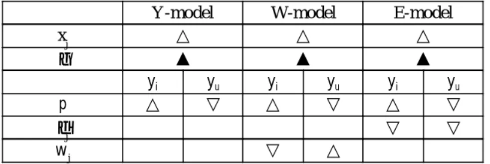
From the above we can see that each model has different parameters associated with the input sources, which drive the activation of the model up toward (or back down toward) the maximum (or the minimum). We begin our study with a few basic properties of the fuzzy γ -models. A number of important properties of the fuzzy γ -models can be associated with the basic fuzzy set theoretic connectives. Table 1 shows some of the properties with respect to output values.
Table 1 Basic Properties of the fuzzy γ -models
The above formulation has the advantage of allowing the parameters to govern the desired behavior of the model instead of requiring knowledge to describe decision process. It also has the characteristic that the final model tends to represent unknown approximated function transparently. These desirable properties provide the flexibility in network implementation.
Y-model W-model E-model
xj △ △ △
γ ▲ ▲ ▲
yi yu yi yu yi yu
p △ ▽ △ ▽ △ ▽
δj ▽ ▽
wj ▽ △
▲monotonical increasing ▼monotonical decreasing
△monotonical nondecreasing ▽monotonical nonincreasing
3. Learning Parameters of the Fuzzy γ-Models
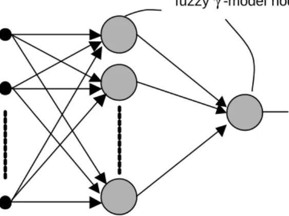
In this section, we describe the multilayer architecture of fuzzy γ-models and derive a gradient descent-based algorithm for learning the parameters. Applying the techniques that have proved successful in the learning algorithms used in neural networks (Rumelhart,1986;Hornik,1989), we present a deviation example in Y-model for parameters learning. The architectural graph shown in Figure 2 illustrates the layout of a multilayer fuzzy γ -model based neural network for the case of a single hidden layer. The input vector consists of n information sources, and an integrating function called fuzzy γ - model that performs the “transfer” function in each neuron. Let us assume that there are n inputs to the model, and the training data for this model consis ts of M sets of inputs x1k....xnk with M corresponding desired outputs d k ( for k = 1, 2, ... M). The back- propagation algorithm is used for the learning process. The learning process is to determine the best set of { p, γ } values for the fuzzy γ-model in such a way that the discrepancy between the desired and actual output behavior is minimized. One measure that is commonly used as discrepancy is the sum of squared error
( )
∑ = ∑ −
=
k k
k k
k y d
E
E 2
2 1 2
1 (8)
where yk denotes the k-th set of final output of the Y-model as follows:
( ) yi yu
y= 1−γ ⋅ +γ ⋅ where
( ) { }i
p
j
p j
i min x min y
y 1 1, 1 1 1,ˆ
/ 1
−
=
−
−
= ∑ (9)
{ }u p
j p j
u min x min y
y 1, 1,ˆ
/ 1
=
= ∑ (10)
Figure 2 Architectural graph of the fuzzy γ -model neural network.
The model is then optimized by minimizing E with respect to the parameters of the fuzzy γ -model. Thus, we update γ value and p value using the following equations based on gradient descent
γ new = γold -
∂γ η1⋅∂E
= γold - η ⋅∑(y −d )∂γ∂y
k
k k
1 (11)
p new = p old -
p E
∂ η2⋅∂
= pold - ( )
p d y y
k
k k
∂
− ∂
⋅
η2 ∑ (12)
where η1 and η2 are suitable positive constants and
i
u y
y y
−
∂ =
∂
γ (13)
( )
( ) { }
{ }
{ } { }
=
≥
=
≥
=
≥
<
∂ <
⋅∂
=
≥
<
∂ <
⋅∂
−
−
<
<
<
∂ <
⋅∂
∂ +
⋅∂
−
−
∂ =
∂
ˆ 0 ˆ 1
ˆ 0 ˆ 1
0
ˆ 0 ˆ 1
ˆ 1 ˆ 0
ˆ 0 ˆ 1
ˆ 1 ˆ 0
1
1 ˆ 0 1
ˆ ˆ 0
1 ˆ
u u
i i
i i
u u
u u
i i
u i
u i
y or y
and y
or y
y or y and p y
y
y or y
and p y
y
y and
p y y p
y
p y
γ γ
γ γ
(14) and
fuzzy γ -model nodes
Input layer hidden layer output layer X1
X2
Xn
y
⋅
∂ =
∂ − ∑
j u
j p j p u u
yˆ ln x p x
yˆ p
yˆ 1
(15)
−
⋅
−
∂ =
∂ − ∑
j i
p j j p
i i
yˆ ln x ) x p (
yˆ p
yˆ 1
1
1
(16) This learning process is repeated until there is no change in γ and p. The choice of η1 and η2 is important and it determines the speed and reliability of convergence (Rumelhart, 1986; Zurada,1992).
4. Simulation Results
In this section, we give two numerical examples to illustrate the characteristics of the fuzzy γ -model neural networks. First we present a simple example that provides a clear training process for the union-like and intersection-like data sets. We also demonstrate that the fuzzy γ -model can be used to implement function approximation in this example. The second example deals with the nonlinearly separable exclusive-OR problem.
Example 1
All of the three fuzzy γ-model were trained using the data sets that used by Keller et al. [Keller,1994]. In all examples, the parameters were initialized as
Y-model : γ=0.5 W-model :
γ=0.5 w1=1.0 w2=1.0 E-model :
γ=0.5 δ1=1.0 δ2=1.0
The parameter p was initialized to be 1.0, 2.0, 5.0, and 20.0 for the three types of fuzzy γ-model operators. We use the gradient descent-based learning algorithm described in Section 3 for parameters learning. The learning process is to determine the best set of {p, γ} values for the fuzzy γ -model in such a way that the discrepancy between the desired and actual output behavior is minimized. As can be seen, the fuzzy γ -model operators give us fairly good responses for function approximation of “union-like” and
“intersection-like”. Table 2 summarized the actual outputs of the experiments.
Table 2 Syntactic data set for example 1 (a) union-like example
input patterns output values
x1 x2 desired values Y-model W-model E-model
0.343 0.123 0.412 0.403 0.409 0.413
0.111 0.999 0.999 0.999 0.999 0.999
0.037 0.222 0.322 0.236 0.322 0.324
0.900 0.200 0.980 0.983 0.981 0.980
(b) intersection-like example
input patterns output values
x1 x2 desired values Y-model W-model E-model
0.343 0.123 0.123 0.103 0.092 0.077
0.111 0.999 0.111 0.111 0.111 0.114
0.037 0.222 0.003 0.003 0.001 0.004
0.900 0.200 0.150 0.200 0.196 0.153
For the union-like data set, the final parameters were as follows:
Y-model p = 1.3643 γ = 0.9994 MSE = 0.0018
W-model p = 1.6330 γ = 0.9986 w1 = 1.0000 w2 = 1.7849 MSE= 0.0000 E-model p = 1.6524 γ = 0.9996 δ1 = 1.0384 δ2 = 0.7582 MSE= 0.0000
In all of the above three cases, the fuzzy γ -models became union-like operators since γ values are high.
For the intersection-like data set, the final parameters were as follows:
Y-model p = 6.4685 γ = 0.0000 MSE = 0.0007
W-model p = 5.7487 γ = 0.0003 w1 = 1.0000 w2 = 1.0284 MSE= 0.0007 E-model p = 7.8791 γ = 0.0041 δ1 = 1.0041 δ2 = 1.1778 MSE= 0.0005
In all of the three cases, the fuzzy γ - models became intersection-like operators since γ values are low. It can be seen that the fuzzy γ -models can be used to implement function approximation in this example.
Example 2. Non-linearly separable examples (The XOR problem)
The second example is based on the exclusive-OR (XOR) problem in which there are two non-linearly separable classes. In particular the pairs (0, 1) and (1, 0) constitute one class and the patterns (0, 0) and (1, 1) constitute the other. This is a traditional example for showing that there exists no single decision plane that can separate these patterns into two classes.
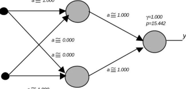
We used a general configuration with two hidden nodes and one output node to approximate the non-linearly separable function. Figure 3 shows the architectural network. Each node in the network represents a single Y-model for which the connections were associated with the degrees of activation of the sources. In traditional feedforward neural networks the weights can be positive or negative, for excitatory or
inhibitory connections, respectively. In fuzzy γ -model neural network, we have tended to take into account both the excitatory and inhibitory in the activation of the node. Without loss of generality, we express the “complement effect” in the connections. Thus, the modified input from source i to fuzzy γ -model node is given by
( i)( i)
i i '
i ax a x
x = + 1− 1− 0≤ai ≤1 (17)
Here, ai refers to the activation from source i, and the input to node has values xi and 1 – xi for ai = 1 and ai = 0, respectively. In general, ai controls the compensatory degree between inhibitory and excitatory. Note also that ai lie in the interval [0, 1].
Figure 3 Configuration of the fuzzy γ -model neural network
At the end of training, the result indicates that the fuzzy γ -model based neural network is able to learn the non-linearly separable decision boundaries very well. We can see that ai = 0 represents the complement set, i.e. ¬xi, of the input source xi. It will tend to inhibit the input sources. Another effect in the fuzzy γ -model is the “degree of compensation’. As the training proceeded, the γ values associated with the hidden nodes gradually decreased toward zero simultaneously whereas the γ value associated with the output node in creased toward one. We can see the γ parameters in Figure 3 as acting as a controller that tends to turn the fuzzy γ -model into an intersection node or an union node in this example. The closer the values of the γ to 1 and 0 the node can be regarded as a pure union and intersection, respectively. Indeed, we can see that the analogous XOR function can be obtained from Figure 3 as
( x1 x2) (x1 x2)
y= ¬ ∧ ∨ ∧¬ (18)
x1
x2
a≅1.000
a≅0.000
γ=0.000 p=11.831
γ=0.000 p=11.831
γ=1.000 p=15.442
y
x1 x2
0.1 0.1 0.1 0.9 0.9 0.1 0.9 0.9
0.9 0.1 0.9
0.1
ydesired yactual
0.105 0.894 0.894 0.105
MSE=0.0003
a≅1.000
a≅1.000
a≅1.000
a≅0.000
This allows the unknown functional relationship in the training data to represent as a transparent neural network configuration. This transparency can provide inside into the nature of the training examples representation, which is useful in the decision making process.
5. Summary
The fuzzy γ -model framework described in this paper illustrates that the fuzzy models can be easily integrated into neural networks for decision function learning. We examined the use of the fuzzy γ-models and their generalizations as neural nodes in network implementation. The proposed method is capable of aggregating information to arrive at appropriate overall decision functions. Network interpretation through this methodology is quite possible. In the empirical experiments, we demonstrated that the proposed network can be used to obtain desired approximations in synthetic decision making problems.
Acknowledgment
This research work was supported in part by the National Science Council under Grant NSC-892218-E-006041, Taiwan.
References
Buckley, J. J. and Y. Hayashi, “ Fuzzy Neural Networks”, in Fuzzy Sets, Neural Networks, and Soft Computing, Eds. by R. Yager and L. Zadeh, pp233-249, 1995.
Chiang, J. -H., " Choquet Fuzzy Integral-Based Hierarchical Networks for Decision
Fodor, J., J.-L. Marichal, and M. Roubens, " Characterization of the Ordered Weighted Averaging Operators", IEEE Trans. Fuzzy Systems, 3(2), 236-240, 1995.
Hirota, K. and W. Pedrycz, “ OR/AND Neuron in Modeling Fuzzy Set Connectives”, IEEE Trans. Fuzzy Systems, 2(2), 151-161, 1994.
Hornik, K., M. Stinchcombe, and H. White, “ Multilayer Feedforward Networks are Universal Approximators”, Neural Networks, 2(5), 359-366, 1989.
Kandel, A., Fuzzy Mathematical Techniques with Applications , Reading, MA: Addison- Wesley, 1986.
Keller, J. and R. Krishnapuram, Z. Chen, and O. Nasraoui, “Fuzzy Hybrid Operators for Network-Based Decision Making", International Journal of Intelligent Systems, 9(11), 1001-1023, 1994.
Klir, G. J. and B. Yuan, Fuzzy Sets and Fuzzy Logic: Theory and Applications , Prentice- Hall, NJ, 1995.
Krishnapuram, R. and J. Lee, " Fuzzy-Connective -Based Hierarchical Aggregation Networks for Decision Making", Fuzzy Sets and Systems, 46, pp11-27, 1992.
Kruse, R., J. Gebhardt, and F. Klawonn, Foundations of Fuzzy Systems , John Wiley &
Sons, Chichester, England, 1994.
Pedrycz, W., Fuzzy Sets Engineering, CRC Press, Boca Raton, 1995.
Rumelhart, D.E. and J.L. McClelland, Parallel Distributed Processing , I, MIT Press ,1986.
Takagi, H., N. Suzuki, T. Koda, and Y. Kojima, “ Neural Networks Designed on Approximate Reasoning Architecture and Their Applications”, IEEE Trans. Neural Networks, 5, 752-760, 1992.
Yager, R. R. , " Aggregation Operators and Fuzzy Systems Modeling", Fuzzy Sets and Systems, 67, pp129-146, 1994
Zimmermann, H. -J. , Fuzzy Set Theory and Its Applications, Kluwer-Nijhoff, Boston, 1991.
Zurada, J. M., Introduction to Artificial Neural Systems, West Publishing: St. Paul, MN, 1992.